Pulse Train Fx-LMS Algorithm for Drive File Identification

Abstract

A novel time-domain algorithm is proposed in this paper for the iterative estimation of drive files. A drive file is a synchronized batch of dynamic time series commands that are simultaneously sent to one or more actuators in a test rig that is designed for service environment replication (SER). When drive file commands are input to an SER test rig, the response of the article under test is similar to what was measured in a service environment. The proposed Pulse Train Filtered-X Least Mean Square (PT-Fx-LMS) algorithm is based on methods developed for active noise and vibration control (ANVC). A time-domain PT-Fx-LMS algorithm is shown through several simulation studies to rapidly converge to a dynamic solution in a small number of iterations for a one degree-of-freedom nonlinear suspension. The PT-Fx-LMS algorithm is also shown to enable targeted iteration over isolated time slices within the data set, which challenges conventional frequency-domain techniques.

1. Introduction

Service environment replication (SER) refers to the process of using test machines to apply controlled dynamic loads to test articles in order to replicate operating conditions that the article was designed for. Some examples of SER test rigs include shock dynamometers, flat-track tire test rigs, driving simulators, single- or multi-post dynamic shaker rigs, and multi-axis shaker tables. SER testing enables repeatable response data to be generated for cost-effective and efficient optimization, performance, and/or durability studies. For example, it is well known that tuning the suspension stiffness and damping will significantly impact tire grip on a race car. The indoor laboratory testing of suspension components and sub-assemblies, wheels, brakes, steering systems, seats, engine parts, etc. are commonplace in the modern automotive industry [1,2], and more recently, the full-scale dynamic testing of an entire vehicle has been used to analyze the dynamic motions of vehicle and/or suspension components for ride, handling, and durability studies [3,4,5,6]. The slow, laborious approach to maximizing grip would be to instrument a vehicle, make incremental changes to the suspension, test the vehicle in its actual service environment, post-process the data, then repeat the process until a desired grip was obtained. This process is clearly more efficient when implemented on an SER test rig in a controlled environment [7,8,9].

In order to take advantage of the benefits of SER testing, these test machines typically require a method for synthesizing command input signals that cause one or more measured responses to closely match desired target sensor responses, such as what was measured in an actual service environment. The set of command input signals that are applied to the test machine is referred to here as a drive file, and the process of determining a suitable drive file for a particular SER application is known as drive file identification (DFID). A drive file is a synchronized batch of dynamic time series commands that are sent to the actuators of the test rig, such that the response of the article under test is similar to what is measured in a service environment. Once a suitable drive file is generated, it can be played out many times with different physical setup combinations while recording all pertinent dynamic motions on a SER test rig [3].

Cryer et al. [10], Barber [11], and Lund [12] described some common DFID algorithms for SER applications based on frequency-domain iterative searches. These techniques necessarily assume linearity in the dynamic system, which is frequently a poor assumption that can either lead to the divergence of the iterative process or exceptionally large amounts of iteration time [13]. This condition generally requires highly skilled engineers to manually “guide” the iteration process.

Several frequency-domain wave form synthesis methods have been proposed for DFID by filtering the response error through an inverse linear frequency response model to iteratively estimate the drive file in a batch process [11]. Such techniques also require a linear frequency response model of the multi-input multi-output (MIMO) dynamic system that is accurate over a frequency range covering the spectral energy in the target data, typically from DC to some finite bandwidth [14,15]. Relatively high coherence (i.e., >0.75) between each sensor and at least one actuator are required for this linear model to be usable. A variety of system identification methods are available for generating the inverse linear model [11,12,16,17]. The identification method discussed by [18] extends the use of inverse linear models for DFID to account for the nonlinearities inherent in a vehicle simulator setup. Internal model update methods based on predicted and measured responses on the test rig [19] or tuning the inverse model in the frequency domain based on a local linearization approach were found to be suitable only for diagonal or weakly coupled systems. Cuyper et al. [20] presented an augmented, real-time, mixed sensitivity $H_{\infty }$ feedback controller, but it has limited performance in cases where the system model has delays or non-minimum phase zeroes. Several time-domain based methods have also been proposed using ARMAX models with exogenous inputs that allow direct inversion [21], such as a Multivariable Output-Error State Space (MOESP) Subspace identification method which frames the DFID problem as a state reconstruction problem solved using the Kalman filtering framework [22] and other online methods like adaptive inverse controllers [23], minimal control synthesis algorithms [24], MRAC [25], etc. However, these often carry the risk of parameter drift, control saturation, and damage to actuators.

MIMO feedback linearization has also been shown to successfully drive sensor responses on a test rig to track desired target responses [26]; however, in this type of solution, the dynamics of the test article would be inside the loop and, therefore, dependent on the feedback loop, which, of course, would not be present in the actual application. Testing with feedback linearization in the loop would necessarily alter the dynamics of the test article, thus rendering any SER test results unusable because they would not be representative of the actual test article under realistic operating conditions.

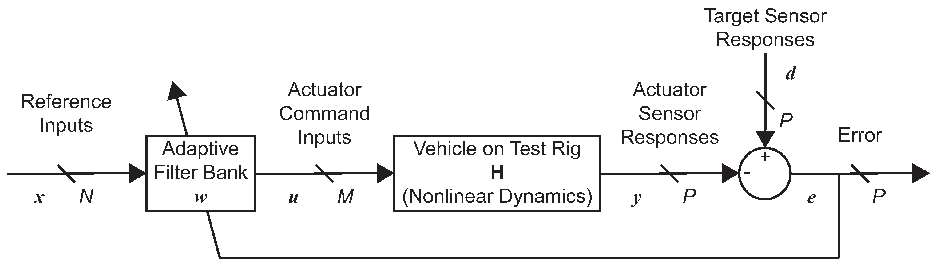
A novel time-domain approach is proposed in this paper for the iterative estimation of drive files. The use of adaptive time domain algorithms is known to be more robust to a wider class of nonlinearities with improved modeling performance, better control over inversion algorithms, and the faster convergence of drives that produce acceptable target responses on test rigs. A time domain-based DFID method would also serve the requirement to select unique convergence rates over different time intervals in a test sequence for which the conventional frequency-domain iterative methods show poor performance. The initial driving factor for this approach was the recognition of the DFID block diagram as a representation of the active noise and vibration control (ANVC) dynamics associated with using secondary path inputs to cancel noise and/or vibration caused by a primary path [26,27]. Even though the block diagram is essentially the same for both ANVC and DFID, the nomenclature, objectives, causality, and known solution approaches have significant differences. More importantly, there are no known control solutions from ANVC which can directly be applied to the DFID problem. Even with this apparent limitation, we will show how the proposed approach can exploit the MIMO ANVC architecture as indicated in Figure 1. We first start with a brief overview of the standard ANVC control block diagram.

For MIMO ANVC applications, the signal $\mathbf{d}$ in Figure 1 represents a primary disturbance noise and/or vibration field measured by P sensors, and the signal $\mathbf{y}$ represents the secondary noise and/or vibration field created by M control actuators to cancel the disturbance. The symbol $\mathbf{w}$ in Figure 1 represents a bank of dynamic filters, typically Finite Impulse Response (FIR) filters, whose coefficients are updated in response to the measured error signals. The signal $\mathbf{x}$ represents a set of N reference inputs, which, for ANVC applications, must be mutually independent and highly correlated to the primary disturbance $\mathbf{d}$ [26,27]. The signal $\mathbf{u}$ contains the outputs from the bank of adaptive filters in response to the inputs $\mathbf{x}$. Note that if the reference inputs are chosen to be the target sensor responses where $N=P$, or a time-advanced version of them, $\mathbf{x}\left(t\right)=\mathbf{d}(t-\tau )$, then the converged filter bank $\mathbf{w}$ represents an approximation to the dynamic pseudo-inverse of the nonlinear system $\mathbf{H}$ [11,12,23,27].

Although both ANVC and DFID seek to drive the output error to zero, or to the theoretical lower bound, ANVC applications require the real-time determination of the control inputs, whereas the command inputs resulting from DFID can be synthesized offline and played out in real-time as a batch that is synchronized with the target data.

For ANVC applications, the adaptation process is typically some form of a gradient descent algorithm, such as least mean squares (LMS). One common gradient-descent adaptation solution developed for the block diagram structure in Figure 1 is known as the Filtered-x LMS (Fx-LMS) algorithm [27,28]. Most commercially available ANVC systems today only operate on periodic or narrow-band wave forms. Even though the structure of Figure 1 with Fx-LMS adaptation can theoretically be used with broad-band signals, such configurations have had very limited success largely because broad-band ANVC applications have a number of severe physical restrictions such as high modal density, the existence of a sufficiently correlated upstream reference signal, high computational burden, or zones of silence with limited spatial extent [28,29].

For the DFID problem, virtually all responses generated from rich excitations will result in target signals that have broad-band spectral content, thus making DFID a technically challenging problem. Existing methods from ANVC cannot be used directly.

The proposed Pulse Train Fx-LMS (PT-Fx-LMS) algorithm will use an innovative reformulation of an ANVC adaptation algorithm that was originally developed by Elliott and Darlington [30] for a completely different application: removing harmonic synchronously sampled interferences from signals. A review of the existing literature indicates that this algorithm has not been extended to generate control inputs for MIMO dynamic systems or to broad-band signals. The strength of the proposed algorithm is derived from its ability to robustly synthesize arbitrary broad-band time-domain wave forms. Using the newly proposed formulation, this synchronous harmonic algorithm provides the basis for a new candidate general purpose DFID solution.

To establish proof-of-concept, the performance of the PT-Fx-LMS algorithm is demonstrated using a simple single-input single-output (SISO) nonlinear dynamic system example: a nonlinear suspension spring supporting a one-DOF vehicle on a test rig. Several case studies illustrate the performance of the PT-Fx-LMS algorithm in comparison with a conventional DFID implementation.

2. Pulse Train Fx-LMS Algorithm

For an SISO dynamic system, and with reference to Figure 1, we have $M=P=1$. Similar to the original development for harmonic synchronous interferences by Elliott and Darlington [30], the novel aspect of the proposed formulation is to select the reference input ${\mathbf{x}}_{\mathbf{k}}$ to be a unitary pulse train (PT) sequence whose period is equal to the length K of the target data set.

$$\begin{array}{c}\hfill \begin{array}{cc}\hfill {\mathbf{x}}_{\mathbf{k}}& ={\left[\begin{array}{ccccc}{x}_1& \cdots & x_q& \cdots & x_K\end{array}\right]}^T\hfill \\ \hfill x_q& =\left\{\begin{array}{cc}1\hfill & \mathrm{if}q=k\hfill \\ 0\hfill & \mathrm{if}q\ne k\hfill \end{array}\right.\hfill \end{array}\end{array}$$

(1)

This unique choice of reference input enables the interpretation of the target response vector $\mathbf{d}$ as an FIR filter whose coefficients are identical to the measured set of target data. Clearly, the output of this FIR filter excited by the unitary pulse train sequence is the target response ${\mathbf{d}}_{\mathbf{k}}={\left[\begin{array}{ccccc}{d}_1& \cdots & d_k& \cdots & d_K\end{array}\right]}^T$. Now, referring to Figure 2, we define a second FIR filter ${\mathbf{w}}_{\mathbf{k}}={\left[\begin{array}{ccccc}{w}_1& \cdots & w_k& \cdots & w_K\end{array}\right]}^T$, which is exactly the same length as the target data set. After convergence, and by construction, the coefficients of $\mathbf{w}$ will be the final drive file.

An adaptive process is needed to dynamically update the FIR filter coefficients in $\mathbf{w}$. Following the practice from ANVC [27], a scalar quadratic cost function, J, of the output error is established, which is to be minimized over time.

$$\begin{array}{cc}\hfill {\mathbf{e}}_{\mathbf{k}}={\mathbf{d}}_{\mathbf{k}}-{\mathbf{y}}_{\mathbf{k}}& ={\left[\begin{array}{ccccc}{e}_1& \cdots & e_k& \cdots & e_K\end{array}\right]}^T\hfill \end{array}$$

(2)

$$\begin{array}{cc}\hfill J& =E\left\{\sum _{k=1}^K{e_k}^2\right\}\hfill \end{array}$$

(3)

where $E\{•\}$ is the expectation operator, and ${\mathbf{y}}_{\mathbf{k}}={\left[\begin{array}{ccccc}{y}_1& \cdots & y_k& \cdots & y_K\end{array}\right]}^T$ is the response vector obtained from the dynamic plant to control input ${\mathbf{u}}_{\mathbf{k}}={\left[\begin{array}{ccccc}{u}_1& \cdots & u_k& \cdots & u_K\end{array}\right]}^T$. A fundamental assumption in the Fx-LMS algorithm derivation is that the FIR filter ${\mathbf{w}}_k$ can be commuted with the plant dynamics, which, of course, requires linearity in the plant as stated by Widrow and Stearns [27]. In general, commutability will not generally be possible for nonlinear systems. Disregarding this fact for the moment and ignoring the nonlinear portion of the dynamics, a Q-coefficient linear FIR filter ($\widehat{\mathbf{G}}={\left[\begin{array}{cccc}{\widehat{g}}_0& {\widehat{g}}_1& \cdots & {\widehat{g}}_{Q-1}\end{array}\right]}^T$) can be constructed to model the dynamic plant around an operating point. The application of the conventional Fx-LMS algorithm in Figure 2 yields the gradient descent method for updating the FIR filter coefficients [27]:

$${\mathbf{w}}_{k+1}={\mathbf{w}}_k+\mu e_k{\mathbf{r}}_k$$

(4)

where ${\mathbf{w}}_k$ is the entire K-coefficient FIR filter at time step k, $\mu$ is a small positive constant known as the step size, which controls the convergence rate, $e_k$ is the instantaneous scalar output error, and ${\mathbf{r}}_k$ is a vector of length K constructed as the buffered output of the linear impulse response model $\widehat{\mathbf{G}}$ due to the reference input ${\mathbf{x}}_{\mathbf{k}}$. It has been shown that the step size $\mu$ depends on the inverse of the signal power [27]; however, it is also known that these relationships do not yield precise constraints. For this study, the step size $\mu$ was chosen via trial-and-error to ensure stability and the fast convergence of the error to zero in a reasonable number of iterations. The simplicity of the unitary pulse sequence, combined with the novel structure of the $\mathbf{w}$ vector representing the actual drive file and the linear FIR model $\widehat{\mathbf{G}}$, can now be exploited to yield a remarkable simplification of the adaptation law given by the following:

$$\begin{array}{c}\hfill {\left[\begin{array}{c}{w}_q\\ w_{q-1}\\ ⋮\\ w_{q-Q+1}\end{array}\right]}_{k+1}={\left[\begin{array}{c}{w}_q\\ w_{q-1}\\ ⋮\\ w_{q-Q+1}\end{array}\right]}_k+\mu e_k\left[\begin{array}{c}{\widehat{g}}_0\\ {\widehat{g}}_1\\ ⋮\\ {\widehat{g}}_{Q-1}\end{array}\right]\\ \hfill \mathit{where}\mathit{q}=\mathit{k}\mathit{mod}\mathit{K}\end{array}$$

(5)

where q is an index into the $\mathbf{w}$ vector at the current time step k. It can be seen from the equation that at any given time step, only a subset (Q-coefficients) of the overall weight vector $\mathbf{w}$ is required to be updated, and the gradient is simply the FIR filter $\widehat{\mathbf{G}}$ multiplied by the instantaneous error. This update law makes physical sense in that the input action at any time step will influence the response that lasts for the duration of the impulse response of the plant. By construction, each weight $w_q$ represents an input action at the qth time step.

3. Nonlinear Simulation Model

The nonlinear time-invariant dynamics of the vehicle on the test rig are given by the symbol $\mathbf{H}$ in the previous block diagrams. The nonlinear model $\mathbf{H}$ can be represented as a set of linear dynamics interconnected with a nonlinear feedback path, as indicated in Figure 3. The representation in Figure 3 reflects the common engineering practice and desire to develop linear models of the nonlinear system while still acknowledging the fact that nonlinearities are present in the dynamics. Notice that the block diagram structure in Figure 3 is actually a generalization of the Lur’e problem described in Vidyasagar [31].

The linear continuous-time model is represented as a state-space representation in Equation (6), the first-order differential equations of the system in Equation (7), and the state-space representation in Equation (8), where all the memory-less nonlinearities are modeled as exogenous inputs to the linear model.

$$\dot{\mathbf{z}}=\mathbf{Az}+\mathbf{Bu}+\left[\begin{array}{cc}\mathbf{I}& \mathbf{0}\end{array}\right]{\mathbf{u}}^{\prime }$$

(6)

$$\begin{array}{c}\hfill \begin{array}{cc}\hfill \dot{\mathbf{z}}& =\mathbf{Az}+\mathbf{Bu}+\mathbf{f}(\mathbf{z},\mathbf{u})\hfill \\ \hfill \mathbf{y}& =\mathbf{Cz}+\mathbf{Du}+\mathbf{g}(\mathbf{z},\mathbf{u})\hfill \end{array}\end{array}$$

(7)

$$\begin{array}{cc}\hfill \iff \left[\begin{array}{c}\mathbf{y}\\ {\mathbf{y}}^{\prime }\end{array}\right]& =\left[\begin{array}{c}\mathbf{C}\\ \mathbf{I}\\ \mathbf{0}\end{array}\right]\mathbf{z}+\left[\begin{array}{c}\mathbf{D}\\ \mathbf{0}\\ \mathbf{I}\end{array}\right]\mathbf{u}+\left[\begin{array}{c}\left[\begin{array}{cc}\mathbf{I}& \mathbf{0}\end{array}\right]\\ \mathbf{0}\\ \mathbf{0}\end{array}\right]{\mathbf{u}}^{\prime }\hfill \\ \hfill {\mathbf{u}}^{\prime }& =\left[\begin{array}{c}\mathbf{f}(\mathbf{z},\mathbf{u})\\ \mathbf{g}(\mathbf{z},\mathbf{u})\end{array}\right]=\left[\begin{array}{c}\mathbf{f}\left({\mathbf{y}}^{\prime }\right)\\ \mathbf{g}\left({\mathbf{y}}^{\prime }\right)\end{array}\right]\hfill \end{array}$$

(8)

It is important to note that the nonlinear model representation above is only used in the simulation study to provide outputs from the nonlinear dynamics. This particular nonlinear architecture lends itself nicely to discretization, which, without the loss of generality, more conveniently integrates with the inherently discrete-time PT-Fx-LMS adaptation law. Note that neither this model structure nor the explicit form of the nonlinearity were explicitly used in the PT-Fx-LMS algorithm.

The performance of the proposed PT-Fx-LMS algorithm is demonstrated using a single-input single-output (SISO) nonlinear dynamic system example. As indicated in Figure 4, the dynamic system is a primary suspension with a stiffness that is modelled with a cubic nonlinearity. The nonlinear dynamic system is linearized at an operating displacement of $y_B$ to obtain the Jacobian linear model $\mathbf{G}$ in Figure 3. The operating displacement $y_B$ represents the static ride height due to gravity. This is a reasonable representation of a spring that achieves a binding condition for spring compressions greater than $y_B$.

$$\begin{array}{c}\hfill \begin{array}{c}\hfill m\ddot{y}+b\dot{y}+F_s\left(y\right)=F\left(t\right)\end{array}\end{array}$$

(9)

In the context of this example, the objective of DFID is to synthesize a command sequence for the applied force $F\left(t\right)$ such that the output displacement $y\left(t\right)$ tracks a desired target data set. For the above-described simulation, the parameters of the system and the constitutive equation of the nonlinear spring are given in

Table 1. System parameters for described simulation.

Parameter	Details	Units
m	200	kg
b	3000	Ns/m
$F_s$	$1.2\times {10}^7$$y^3+$$1.2\times {10}^6$$y^2+$$9.5\times {10}^4$y	N
$y_B$	$-0.05$	m
$k_J$	$6.5\times {10}^4$	N/m

. This is an example of a duffing oscillator. The operating point around which the nonlinear model is linearized is $y_B$, and the linearized spring model, $\mathbf{G}$, has a Hooke’s constant given by $k_J$. A smooth, cubic, nonlinear spring is considered for the test benches presented in this study, but there can be other classes of nonlinearities like piece-wise nonlinear systems that can also be considered for simplified suspension models as above.

4. Results and Discussion of Performance Evaluation Case Studies

In all the case studies below, the desired target data set was chosen to be an experimental displacement measurement from an actual vehicle suspension collected during a 25 s lap around a test track. The data were acquired at a sample rate of 1000 Hz. A series of simulation case studies was performed to document the proposed PT-Fx-LMS DFID method. The results from three of these studies are presented below to illustrate the features of the method operating in the more typical batch mode.

For the proposed time domain PT-Fx-LMS method, the linear dynamics $\widehat{\mathbf{G}}$ must be estimated for implementation. For the purpose of simulation, as described in Section 3, the linear dynamics $\mathbf{G}$ were estimated through the Jacobian linearization of the nonlinear spring model at $y_B$. A band-limited excitation that produces a response from the system around the operating point $y_B$ was designed, and the actual response of the nonlinear dynamic system was obtained for this particular excitation. An adaptive Least Mean Squares System Identification algorithm, as described by Widrow and Stearns [27], was used to estimate a Q-coefficient FIR filter representing $\widehat{\mathbf{G}}$. For the spring–mass system chosen in this paper, a 1000 coefficient FIR filter $\widehat{\mathbf{G}}$ was determined to capture the linear dynamics of the system.

A useful metric to compare the adaptation performance is the normalized error energy (NEE), which is defined for each batch loop iteration, i, as

$$NE{E}_i=\frac{{{\mathbf{e}}_{\mathbf{i}}}^T{\mathbf{e}}_{\mathbf{i}}}{{\mathbf{d}}^T\mathbf{d}}$$

(10)

where ${\mathbf{e}}_{\mathbf{i}}$ is the entire error signal vector at the end of each batch loop iteration i. NEE is a normalized measure of the mean square error averaged over the entire batch of data and is usually expressed on a decibel scale. NEE essentially measures how close the SER test rig response data are to the desired target data, and the same metric is also used to characterize the derived FIR model using the LMS system identification method, as shown in Figure 5, which shows the modeling performance for both the purely linear plant with the spring constant $k_J$ and the cubic nonlinear plant characterized by the force curve given by $F_s$. The difference in modeling quality is also useful to gauge the robustness of the proposed DFID method in the presence of modeling errors. The model identification result expressed in NEE is also presented for the conventional frequency-domain H₁ estimation method [32] using the same band-limited excitation to illustrate the improved modeling performance of the iterative adaptive filtering-based method.

As with most real-world DFID processes, the adaptive algorithm is terminated when the error is smaller than a predefined threshold. For the case studies described in this paper, the threshold was set to a 40 dB reduction in the NEE.

4.1. Setup of Comparative Method

The performance of the proposed PT-Fx-LMS method is compared against an existing DFID formulation that forms the basis of commercial DFID solutions like MTS Remote Parameter Control. While the exact formulation is proprietary, the workflow of the DFID process and the adaptive algorithm used to arrive at a suitable drive file is well documented in [11]. The process involves filtering the target response through an inverse frequency response model of the plant to derive the drive file. This initial drive file is played through to the actual plant and the response is compared to the target response. The error between the two is used to calculate the drive file correction and added to the previous drive file in an adaptive process to drive the response error to zero or to an acceptable lower bound defined by a threshold appropriate to the application. Many formulations exist for this identification of the inverse linear model, including conventional techniques of calculating an inverse FRF of a linear system model derived from a system identification procedure on the nonlinear plant, the direct calculation of the forward linear model via the linearization of the nonlinear model equations followed by conventional inversion, etc. In this paper, a time-domain delayed adaptive inverse method described by [23] is used to calculate the static inverse linear model using the previously described $\widehat{\mathbf{G}}$ forward linear model. The inverse linear model identified is a 5000 coefficient FIR filter, with a 1000 coefficient delay, and it is observed to converge within 100 iterations with a white noise reference input for the identification process and a choice of iteration coefficient that maintains stability and provides necessary performance and fast convergence. Further insight into the choice of the iteration coefficient that ensures stability and enhances convergence rate for a conventional DFID process for a nonlinear system using remote parameter control is provided by Li and Zhang [33].

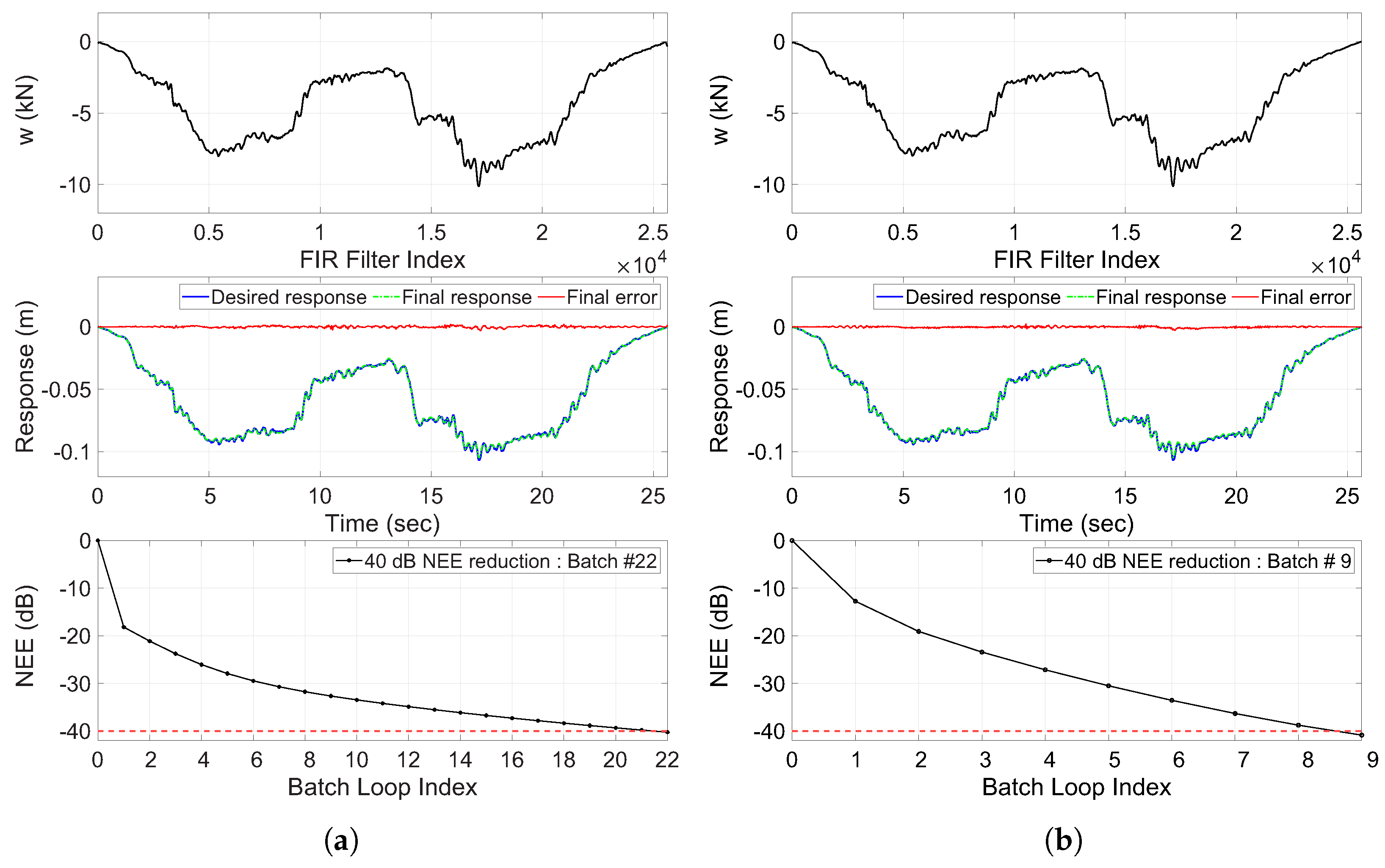
4.2. Case Study 1

In the first study, the drive signal was initialized at zero and the adaptation step size was chosen to be relatively conservative to balance stability and fast convergence; in this case, $\mu =$$4.8\times {10}^9$. At the end of each batch loop, the final drive signal was used as the initial drive signal for the next batch loop. The adaptive algorithm was run until the NEE reached the threshold of 40 dB reduction. In Figure 6b, the first subplot presents the final drive file after the final batch loop adaptation. The response of the dynamic system to this final drive file is given in the second subplot along with the error between the actual and desired responses. The third subplot shows the reduction in the NEE throughout the batch iterations of the adaptation process. Since the purpose of the DFID process is only to synthesize control inputs that would generate a response as close to the desired response as possible, the convergence of the algorithm is not shown in Figure 6. Simulations were nevertheless carried out for a large number of batch loops to check for the stability and convergence of the algorithm, and it was found that for the system under test and choice of step size used here, the NEE converges to −70 dB after approximately 2000 iterations, which is far greater than what would be feasible due to time and cost constraints on a real-world test rig for the DFID process.

As can be seen, at the end of the simulation presented, the proposed method achieves a final response which is very close to the desired response with a low misadjustment, which, as defined by Widrow and Stearns [27], is a dimensionless measure of the excess mean square error caused by gradient estimation noise relative to the minimum mean square error produced by an optimal Weiner filter. Widrow and Walach [23] showed that misadjustment increases with an increase in the speed of adaptation and/or the number of filter coefficients. The parameters for both the proposed time-domain PT-Fx-LMS method and the conventional DFID process described in Section 4.1, with its results shown in Figure 6a, were tuned in order to achieve rapid reduction in NEE to reach the error threshold in the least number of iterations. In the DFID process, each simulated batch loop corresponds to a physical test on the SER test rig (‘Batch Loop index’ in the subsequent figures), and there is a strong desire to minimize the number of experimental tests in order to save time and money. Considering the least squares nature of the adaptive algorithm, the presence of measurement noise is known to only increase the final achievable misadjustment level and is not considered in these validation simulation test benches.

The reduction in the NEE is plotted in Figure 7 along with the maximum absolute response error within each batch loop iteration. As can be seen, the performance of the proposed method, with no actuator authority limitations, is demonstrably good for the parameters used in this simulation study in the sense that it reaches the 40 dB NEE reduction threshold with fewer iterations, at 9 iterations compared to 22 iterations for the conventional DFID method.

Figure 8a presents the progression of the response measured at the end of batch iteration in the time domain, and Figure 8b presents the similar progression using the power spectrum, computed using a window size of 8192 samples and 50% overlap. The least squares adaptive algorithm always targets the peaks in the spectrum first in order to drive the MSE to zero. The output response obtained from the final drive derived using the PT-Fx-LMS method converges to use most of the batch iterations to attenuate the error when the response is lower than the binding point of the nonlinear spring where the force curve exhibits the most stiffening property. In the spectrum, the actual response deviates the most from the target response in the 7–15 Hz range, which has a spectrum magnitude of at least 25 dB smaller than the peak for the model and target data considered in this study. Targeted improvements can be made by increasing the coherence of the identified model in the required frequency bands via excitation shaping during the system identification step.

Although the proposed method in this paper does show performance improvement over the conventional DFID method, it is important to note that such a result is to be expected because the conventional DFID method heavily depends on the accuracy of the inverse linear model that is generated, in this case, an inverse of a forward model $\widehat{\mathbf{G}}$ of the nonlinear plant using an adaptive inverse method, instead of conventional FRF inversion methods. With the system identification process for the forward model $\widehat{\mathbf{G}}$ and the subsequent inversion process being tuned for best performance, it can also be expected that the two DFID methods compared here would show much more similar performances for linear plants (a linear spring in Figure 4) under study or for less harsh nonlinearities. Such a scenario was investigated further by considering a linear spring model for the plant, where the spring stiffness is given by the Jacobian spring model, $k_J$, from Table 1 and using the same simulation parameters as discussed above. With much more accurate models derived for this linear plant, the conventional DFID method was able to reach the 40 dB NEE reduction threshold in just six iterations, whereas the proposed PT-Fx-LMS method needed eleven iterations to reach the same level of misadjustment. This shows that the proposed method, while being comparable and usable but not outperforming conventional DFID methods for simple linear systems, can be extremely powerful for nonlinear systems, as most real-world dynamical systems are.

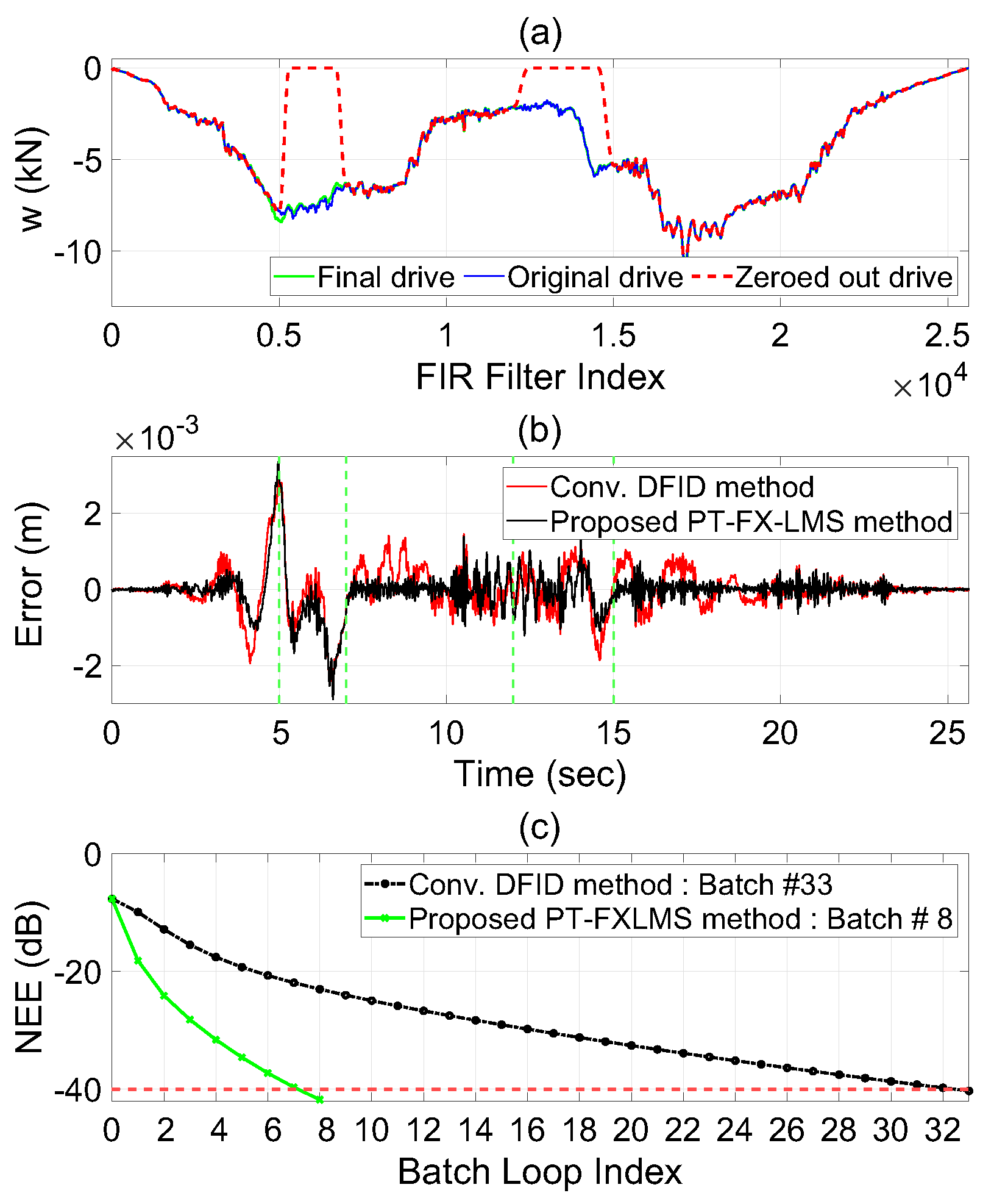
4.3. Case Study 2

In many practical DFID applications, it is often useful or necessary to have the ability to fine-tune sections of the drive file by focusing on specific intervals in time. Frequency-domain techniques typically have difficulty focusing on select time intervals without perturbing the response outside those intervals. To illustrate the ability of the PT-Fx-LMS DFID method to focus on specific time intervals, another series of case studies was performed.

In this first time-slice study, the optimal drive signal from the previous evaluation (Figure 6) was artificially perturbed by zeroing out the drive signal over two time intervals: 5–7 s and 12–15 s. This perturbed drive signal was then used as the initial control sequence, and the adaptation process was iterated to see if the drive file would return to the original solution. Partially zeroing out the control sequence in intervals is an extreme test to evaluate how well the algorithm works within time slices while also not affecting the converged drive file outside these regions. In order to avoid sharp discontinuities in the initial drive file that could lead to large spikes in actuator authority, the transitions at the intervals were smoothed. The simulations were similarly stopped when an NEE threshold of −40 dB was achieved.

As can be seen from the results in Figure 9, the proposed PT-Fx-LMS algorithm returned to a solution with low misadjustment and without significantly affecting the response outside the intervals of interest after only nine batch loop iterations. The largest magnitude of errors, which are still an order of magnitude smaller than the response, were observed at the edges of the perturbation window without increasing the errors significantly outside these intervals. This clearly demonstrates that the response of the proposed method in one time interval is relatively independent of the response in another. It can also be seen in Figure 9b that the conventional DFID method yields larger magnitude errors even outside the bounds of the perturbed intervals (see time interval 7–10 s and 15–20 s) despite the adaptation for both methods starting from the same perturbed drive signal. The error energy comparison also shows that the proposed PT-Fx-LMS method descends to the threshold NEE much quicker using the same adaptation parameters as in Case Study 1.

4.4. Case Study 3

As an extension of the previous case study, a more extreme perturbation test was performed in which the original optimal final drive from Case Study 1 (Figure 6) was chosen to be the initial drive signal. However, for this study, the target response was zeroed out over the same two time intervals: 5–7 s and 12–15 s. As in Case Study 2, the transition in the interval was smoothed to prevent large spikes in the response or actuator authority. This is an intentionally contrived example whose sole purpose is to illustrate the capability of the method. The simulations were similarly stopped when the NEE threshold of −40 dB was achieved.

As can be seen from Figure 10, the PT-Fx-LMS algorithm yields a response from the actual dynamical system with a small mean squared error at the end of simulation, much fewer iterations, and virtually no impact on the response outside the perturbed intervals, except around the boundaries of the intervals. On the other hand, the conventional DFID method produces larger disturbances in the response outside the perturbed intervals, as can be seen in the error signals in Figure 10b between 7–10 s and 15–20 s, and achieves the threshold NEE at a slower rate, as can be seen in Figure 10c.

In both Case Studies 2 and 3, the PT-Fx-LMS adaptation process was iterated over the entire time series without a priori knowledge of the two perturbed intervals. The unique structure of the PT-Fx-LMS algorithm enables a user to specify the limits of one or more time slice intervals within which the adaptation will occur. Outside these time slice intervals, the adaptation will be suppressed. This allows an even more computationally efficient implementation without any negative impact on the resulting drive file identification.

5. Conclusions

A new algorithm has been proposed for the identification of drive files for service environment replication applications. The proposed Pulse Train Fx-LMS algorithm is derived from a synchronous ANVC adaptive filtering algorithm that is modified to handle the broad-band drive file identification application for nonlinear plants. The two key modifications that enable PT-Fx-LMS to be useful for DFID applications are as follows: (1) the use of a unitary pulse train reference input of the same length as the batch target data set, which results in (2) a simplified adaptation methodology.

The PT-Fx-LMS algorithm was validated on a simple but representative SISO nonlinear suspension using actual suspension displacement time series data from a race car. In addition to demonstrating the iterative operation of the proposed algorithm, its performance was evaluated and compared against a conventional drive file identification method. The linear model used by the PT-Fx-LMS algorithm for the gradient estimate is shown to work quite well for this nonlinear plant example. As is common for conventional Fx-LMS algorithms, linear models used in the gradient estimate are often more than sufficient for nonlinear systems due to the iterative nature of the algorithm.

In order to more thoroughly evaluate the PT-Fx-LMS algorithm, several extreme tests were performed. These tests were created specifically to highlight a common problem that conventional frequency-domain DFID methods have difficulty performing, i.e., focusing the iterative update on isolated time slices in the target data without perturbing the converged response outside those time slices. In one case, the converged control solution was artificially perturbed (set to zero) in two isolated time segments. In the second case, the target data were artificially perturbed (set to zero) in two isolated time segments, and the control solution started from its original converged values. In both cases, the PT-Fx-LMS algorithm was able to converge to the appropriate solution in a small number of iterations without perturbing the existing converged response.

Further methods to improve the DFID are being considered involving completely offline batch iterations using the identified linear model of the plant using finer step sizes in a simulation domain to derive the control sequence that will be played out to the actual plant, with appropriate corrections to the target signal for each simulation sequence being made based on the actual responses measured on the physical test article. Deficiencies in the model could lead to divergence in the adaptation process for which protections can be built in using a termination criterion or using the many variable step size Fx-LMS algorithms available in the literature.

The success of the PT-Fx-LMS algorithm in the simulated case studies above clearly establishes proof-of-concept for this method. The next step is to expand the PT-Fx-LMS algorithm to multiple-inputs and multiple-outputs as well as other classes of nonlinearities that are commonly found in SER applications.