Calculation of Wear of Railway Wheels with Multibody Codes: Benchmarking of the Modelling Choices

Abstract

The numerical simulation of wear of railway wheel profiles can be a game changer in the railway field, as it can drive the planning of wheel re-turning operations, thrust the identification of optimized profiles and evaluate the safety of railway vehicles at the early stages of design. Today, commercial multibody codes are provided with dedicated routines that can evaluate the worn profile shape due to the dynamic behaviour of the vehicle. As the outputs of such modules can depend on different user-selectable parameters and modelling choices, it is vital to assess the capabilities of these codes and get a further understanding of the implemented algorithms. This paper aims to benchmark the effects of different modelling parameters and choices, mainly related to the selected wear law and wheel–rail contact method, on the final wear outputs, with special reference to the wear module provided by the SIMPACK commercial multibody code. A relevant novelty of the paper deals with the benchmarking of the wear algorithm available in the commercial code with in-house wear routines, comparing different strategies and choices for the calculation of wear. This allows us to better understand the most critical differences and modelling issues, as well as to highlight possible improvements in wear algorithms that can lead to enhanced numerical stability. More in detail, this work suggests a change in the wear algorithm that proves to be beneficial to removing local wear peaks produced by numerical sources, which could cause instabilities in the computation.

1. Introduction

As the railway system relies on the wheel–rail frictional contact, the operation of railway vehicles inevitably causes wear of the wheel profiles because of the large forces acting on the contact patch and partial slip originating from the rolling–sliding contact. However, strong deviations of the wheel profiles from the nominal shape can have a negative impact on the vehicle’s dynamic performance [1,2], threatening the running stability and safety (with a possible increase in the derailment risk) as well as the ride comfort [3,4,5,6]. Consequently, the original wheel profile shape is periodically restored through machining operations, which are commonly planned according to a pre-scheduled time or kilometric basis, defined according to previous experience.

The prediction of the wheel profile evolution with numerical codes can be beneficial from different points of view. First, it can assist in the planning of the wheel re-turning operations, leading the path towards condition-based and even predictive maintenance strategies [7]. At the same time, computationally efficient wear simulation tools can be integrated within optimization routines to search for optimal profiles featuring lower levels of wear, hence allowing the extension of the wheel’s expected operating life [8,9]. Moreover, wear numerical tools can be adopted to assess the dynamic performance of railway vehicles with worn profiles at the earliest stages of vehicle design. In fact, the assessment of vehicle running behaviour with numerical simulation as prescribed in Annex T of the EN14363 standard [10] requires that the considered wheel profiles should be appropriate for the reference vehicle, hence for some cases, they could be representative of worn profiles in service.

In view of the higher safety and lower maintenance costs that can be achieved with numerical simulation of wear, railway companies have been showing a growing interest in the numerical simulation of wear during common dynamic operations of railway vehicles, even when not operating on critical sections like turnouts, which has increased studies on the topic [11,12,13,14]. The authors of the present paper surveyed the different strategies for the numerical simulation of wear of railway wheel profiles [15] and found that, currently, the most common solution is based on the interaction between a dynamic simulation module and a wear module. The former is typically a multibody (MB) simulation of the vehicle and track interaction, solving the dynamic equations of motion and the wheel–rail contact problem in each time step, while the latter evaluates the worn material and calculates the worn wheel profile shape.

Although examples of wear simulation tools based on the MB model implemented in in-house codes can be found in the literature [16,17,18], railway companies often adopt commercial MB codes in view of the reliability and previous validation of many built-in elements to simplify the certification and homologation processes. Concerning the wear module, traditionally, it could be written as a separate user routine and integrated within the commercial MB code, while nowadays it can be run in a different computational environment thanks to co-simulation techniques [19]. However, most commercial MB codes are currently provided with built-in wear modules and add-ons, which can be activated to evaluate the worn profile shape in the post-processing stage, thus simplifying the software architecture of the wear computation tool.

Whilst the approach for numerical simulation of wheel profile wear is well described in the literature, the outputs of the wear simulation can be strongly affected by many modelling choices and parameters, even when relying on the wear module of a commercial MB code. Therefore, the present paper aims to benchmark the wear module of the SIMPACK commercial MB code (SIMPACK Wheel Profile Wear module, or SIMPACK wear module in the rest of the paper) and to assess the effects of different modelling choices and parameters. The SIMPACK code is chosen as the reference MB code in view of its leading position in the European market for railway vehicle dynamics simulations. As different commercial codes share similar modelling parameters, the analysis performed in the present work can be easily extended to other MB packages.

For benchmarking purposes, an MB model of the Aln 663 passenger diesel railcar running on a reference track, not corresponding to a real line, is established in SIMPACK 2023.4 [20]. The benchmarking activity is essential to evaluate the reliability of the SIMPACK Wheel Profile Wear module and detect possible improvements for higher stability of the computation. In fact, a major novelty of the work is that it compares the commercial code with the outputs of in-house wear routines, investigating different strategies for the calculation of the amount of worn material, and suggesting changes to the wear algorithm that can be beneficial for the numerical stability of the computation when cascades of wear simulations are launched.

The paper is organized as follows. Section 2 describes the SIMPACK Wheel Profile Wear module and the MB model of the reference vehicle and track, providing information on the user-selectable wheel–rail contact methods. Section 3 presents the results obtained from the numerical simulations launched with SIMPACK and a discussion on the outputs of the benchmarking activity against the results calculated using an in-house MATLAB 2022b wear routine. This allows us to define how SIMPACK spreads the worn material to obtain the wheel profile and to compare the performances of the SIMPACK wear laws for different values of user-tuneable parameters, highlighting possible changes to the algorithm that can lead to an improvement of the stability of the method. Finally, Section 4 summarizes the main outcomes of the benchmarking activity.

2. Model

2.1. Wear Calculation

In this work, the wear of the wheel profile is calculated with both the Wheel Profile Wear module implemented in the SIMPACK commercial code [20] and with a MATLAB in-house wear routine that is compared to the commercial code with the aim of getting a further understanding of the SIMPACK algorithm. Two wear laws are considered to evaluate the amount of worn material produced as the result of vehicle dynamic operation, namely, the energetic law proposed by Krause and Poll (KP) [21] and Archard’s wear law [22,23], in the implementation of the Swedish Royal Institute of Technology (KTH) [24]. In fact, these are the only laws that the user can select when relying on the SIMPACK Wheel Profile Wear module, although many other laws can be found in the literature [25].

Concerning the SIMPACK code, for both laws, the Wheel Profile Wear module uses a global approach, i.e., it calculates the total worn volume for each contact patch and time step, and then it assigns 50% to the wheel and 50% to the rail. According to the KP law, the total worn volume ΔV is proportional to the work of the friction forces W_fric, with a proportionality constant depending on the wear regime, which can be either mild or severe depending on the value of the dissipated power P_fric:

$$\begin{gathered} ∆V=\left\{\begin{array}{c}{C}_m{W}_{fric}, {\displaystyle \raisebox{1ex}{$P_{fric}$}\!\left/ \!\raisebox{-1ex}{$A$}\right.}\le 4 \mathrm{W}/{\mathrm{m}\mathrm{m}}^2\\ C_s{W}_{fric}, {\displaystyle \raisebox{1ex}{$P_{fric}$}\!\left/ \!\raisebox{-1ex}{$A$}\right.}>4 \mathrm{W}/{\mathrm{m}\mathrm{m}}^2\end{array}\right. \\ {P}_{fric}=T\gamma ·v_{roll} \\ T\gamma =\left|F_x\xi \right|+\left|F_y\eta \right|+\left|M_z\phi \right| \\ {W}_{fric}=P_{fric}·∆t \end{gathered}$$

(1)

where A is the contact area; C_m and C_s are the proportionality coefficients for the mild and severe regimes, respectively; Tγ is the wear number; F_x, F_y and M_z stand for the longitudinal force, lateral force and spin moment at the contact patch; ξ, η and φ represent the longitudinal, lateral and spin creepages; v_roll is the rolling speed; and finally, Δt is the time output step, i.e., the inverse of the sampling frequency of the output results.

Conversely, with the KTH wear law, the worn volume is proportional to the normal load N and sliding distance Δs_s through a proportionality constant k_Arch depending on slip speed v_s and average contact pressure p_z:

$$∆V=k_{Arch}\left(v_s, p_z\right)·{\displaystyle \frac{N{\mathsf{\Delta }s}_s}{H}}$$

(2)

where H is the hardness of the softer material, to be expressed in Pa. The proportionality coefficient is typically extracted from experimental maps (see Figure 1), which commonly feature four different regions corresponding to three separate wear regimes, namely, two regions characterized by mild wear (Mild 1 and Mild 2), a region with severe wear and a region dominated by seizure, which is entered when the contact pressure is above a certain threshold.

The implementation within the SIMPACK wear module only allows us to specify the boundaries of each zone (v₁, v₂ and f_p in Figure 1) and a single value of the wear coefficient for each zone. The default values of the boundaries are given in Figure 1. It should be noted that the values applied in SIMPACK should be doubled with respect to the coefficients suggested by KTH researchers [24,26], as the latter are given for the wheel only rather than for the whole wheel–rail system.

Compared to local methods, the global approach used by SIMPACK does not perform a discretization of the contact patch into adhesion and slip regions, hence the worn volume must be spread according to an a priori distribution [27]. As no additional information is provided about the strategy adopted in the algorithm to spread the worn volume along the wheel profile, this work benchmarks the SIMPACK algorithm against an in-house routine that spreads the worn volume according to a semi-elliptic distribution, thus considering the wear depth to be proportional to the Hertzian contact pressure, as stated by

$${∆z}_n\left(s\right)={∆z}_0\sqrt{1-{\left({\displaystyle \raisebox{1ex}{$s$}\!\left/ \!\raisebox{-1ex}{$b$}\right.}\right)}^2}$$

(3)

where Δz_n is the normal wear depth, s is the local lateral coordinate on the contact patch, b is the lateral semi-axis of the ellipse, and Δz₀ is a term that is calculated to keep the same amount of worn volume. This is obtained by ensuring that the following equation is satisfied:

$${\int }_{-b}^b{∆z}_0\sqrt{1-{\left({\displaystyle \raisebox{1ex}{$s$}\!\left/ \!\raisebox{-1ex}{$b$}\right.}\right)}^2}·2\pi R_{cp}(s)\cos \delta \left(s\right)ds={∆V}_w$$

(4)

where R_cp is the wheel radius at the contact point and ΔV_w is the volume removed from the wheel. When referring to an equivalent Hertzian contact patch, assuming a constant value of contact radius and contact angle, the term Δz₀ can be calculated analytically as

$${∆z}_0={\displaystyle \frac{{∆V}_w}{{\pi }^2{R}_{cp}\cos \delta b}}$$

(5)

In this paper, both KP and KTH wear laws are tested and benchmarked. For the KP law, the values of the wear coefficient in mild and severe regimes are taken from the work by researchers from Università degli Studi di Firenze (UniFi) [28], and they are set to Cm = 9.871 × 10⁻¹⁴ m³/J and Cs = 9.871 × 10⁻¹³ m³/J. For Archard’s law, the wear coefficients are taken as the mean value in the range defined for each region by the KTH map, with the application of a reduction factor, to account for the effect of natural lubrication, as suggested by researchers from KTH. The coefficient in each region is provided in

Table 1. KTH wear coefficients adopted in this work.

Wear Region	Wear Coefficient
Mild 1	1.43 × 10−4
Severe	1.00 × 10−3
Mild 2	1.43 × 10−4
Seizure	1.00 × 10−2

.

2.2. Vehicle–Track MB Model

2.2.1. Vehicle Model

The reference vehicle considered in this paper is the Aln 663 passenger diesel railcar, in view of the large wear recorded on the wheels of the vehicles running on the Aosta-Pré-Saint-Didier railway line in the Alpes of Northern Italy. The SIMPACK MB of the Aln 663 diesel railcar was already presented in [19], and it includes 17 rigid bodies and a total of 62 degrees of freedom (DOFs):

• Four wheelsets, each one with six DOFs.
• Eight axle boxes that are only allowed to rotate with respect to their wheelset (1 DOF per body).
• Two bogie-frame bodies, which feature six DOFs each and model the FIAT bogie used on the vehicle.
• Two bolsters that have all six DOFs.
• One carbody with six DOFs.

For bodies with six DOFs, the SIMPACK General Rail Track joint is applied, which enables up to six DOFs defined according to the typical railway reference system, i.e., an s coordinate along the track line, a lateral y coordinate in the local track system, a z vertical coordinate and finally the roll, yaw and pitch rotation along the local track axis directions. The wheel and rail profiles are the standard European profiles, namely the S1002 wheel profile and the UIC60 rail profile.

The MB model is also provided with force elements able to account for the nonlinearities of both suspension stages of the FIAT bogie. The primary suspension system of the FIAT bogie, which connects each axle box to the bogie frame, is obtained with helical springs and a rubber joint mounted in the control arm acting as the axle box guide. The helical springs are modelled with SIMPACK flexicoil elements, which account for the stiffness along the axial (vertical) and transversal directions, as well as for the bending and torsional stiffness, with coupling between bending and shear behaviour. On the other hand, the rubber joint is modelled with the definition of a bushing element with stiffness values in all directions. As for the primary suspension, the secondary suspension of the FIAT bogie mainly includes helical springs, which are modelled with shear spring elements, accounting for the coupled behaviour between shear and bending. The model also includes elements for the simulation of the lateral bumpstops, limiting the carbody lateral displacement, as well as elements to account for the traction rods and lateral/vertical dampers. The connection between each bolster and the coach is modelled with a busing element with high stiffness values in all directions, apart from the yaw stiffness, which is set to zero to account for the cylindrical centerplate.

To ensure that the vehicle follows the desired speed profile, the model includes a dedicated longitudinal force element defined between the carbody and a marker on the track that moves accordingly to one wheelset. In each time step t, the traction force F_trac is calculated as

$$F_{trac}\left(t\right)=K_p·\left[v_{ref}\left(t\right)-v_c\left(t\right)\right]$$

(6)

where v_c is the coach speed, v_ref is the reference speed and K_p is the proportionality constant that is tuned to guarantee a good accordance with the reference speed profile without causing numerical peaks in the traction force itself.

2.2.2. Track Model

As the goal of the present paper is to get a further understanding of the effects of different modelling parameters and choices rather than accurately predict wear on a specific line, the reference track is a simplified track not corresponding to a specific railway line and includes 19 curves with radii in the range of 200–2000 m and a step of 100 m facing the right-hand direction, followed by another set of the same 19 curves in the left-hand direction. Figure 2 shows the curvature along the track, the speed profile followed by the vehicle and the superelevation of each curve. The latter is calculated to ensure values of unbalanced lateral acceleration below the limits prescribed by the Italian railway administration, namely Rete Ferroviaria Italiana (RFI). Please note that in the plots, positive values for curvature and superelevation correspond to right-handed curves, while negative values are used for left-handed curves. The track is modelled as rigid to simplify the analysis of the effects of wear parameters on the predicted wear depth distribution. Similarly, track irregularities are neglected to limit the effect of stochastic parameters in the assessment of the different modelling parameters and choices. Future works could investigate the effect of irregularities as well as flexible track modelling approaches [29].

2.2.3. Wheel–Rail Contact Model

Currently, MB codes solve the wheel–rail contact problem with elastic approaches, i.e., the contact patch area is determined from the penetration of the wheel and rail profiles. This strategy can lead to non-elliptic contact patches; hence, two approaches can be followed to determine the wheel–rail contact forces. The first one relies on turning the non-elliptic patch into an equivalent ellipse, while the second approach is based on advanced algorithms that can deal with non-elliptic patches in the calculation of the forces. Both approaches are directly available in the SIMPACK code, i.e., the equivalent elastic (EE) method, which turns the non-Hertzian area into an ellipse, and the discrete elastic (DE) method, which keeps a non-elliptic patch for the evaluation of the wheel–rail contact forces. Please note that with both methods, the normal and tangential problems are decoupled, as the contact patch size and normal pressure distribution are obtained without considering their dependency on tangential stresses. Kalker’s exact theory (CONTACT algorithm) can solve the wheel–rail contact problem considering the dependency of the normal stresses on the tangential ones, but its computational efficiency is not suitable for long dynamic simulations. The two wheel–rail contact methods are compared in this work in terms of the final wear outputs and computational effort.

The simulations shown in this paper and run with the EE method rely on Kalker’s FASTSIM algorithm [30] to solve the tangential problem, i.e., the identification of the contact stresses and forces. On the other hand, with the DE strategy, a STRIPES-based approach is used to evaluate the tangential stresses and forces [31,32].

It is important to highlight that to avoid high-frequency oscillations in the rail–wheel contact, a damping term is added in the calculation of the total normal force for each time step and contact patch during the simulation, for both EE and DE methods:

$$N\left(t\right)=\max \left\{N_{el}\left(t\right)+N_{damp}\left(t\right),0\right\}$$

(7)

where N is the total normal force, N_el is the elastic component, N_damp is the damping contribution, t is time and a saturation is performed to avoid negative contact forces that would lead the wheel to “stick” to the rail. The EE and DE approaches only differ in that with the DE method, the elastic and damping terms are calculated on each longitudinal slice. The amount of damping can be tuned by the user with the specification of a reference contact damping that corresponds to a reference contact stiffness of 5 × 10⁸ N/m. For other values of contact stiffness, the SIMPACK documentation [20] states that the contact algorithm adjusts the damping value to keep a constant natural damping, as stated by

$$d=d_{ref}\sqrt{{\displaystyle \frac{c}{5·{10}^8}}}$$

(8)

where d is damping, c is the contact stiffness and d_ref is the reference contact damping specified by the user, for which the default value set by SIMPACK is d_ref = 1 × 10⁵ Ns/m.

3. Results

As discussed in the previous section, the wear of the wheel profile eventually depends on the selected wear law and the wheel–rail contact algorithm, which in turn are affected by different modelling choices. This section presents the influence of the selected wear law (Archard or KP), wheel–rail force calculation method (EE or DE method) and contact reference damping on the outputs obtained from the SIMPACK Wheel Profile Wear module. Furthermore, this section benchmarks the results of the SIMPACK wear module with the outputs obtained from the in-house MATLAB wear routine based on the implementation of Equations (3)–(5) to spread the worn volume, thus allowing us to identify possible improvements for the stability of wear algorithms.

Wear is calculated on the wheels of the leading wheelset of the reference vehicle. As similar considerations can be inferred from both the left and right wheels, due to the symmetry of the track curves, results are presented for the right wheel only. The reference quantity chosen to compare the outputs of the wear routines is the normal wear depth, i.e., the wear depth in the normal direction with respect to the profile. In fact, from the distribution of the normal wear depth along the profile, the coordinates of the worn profile can be calculated as

$$\begin{gathered} Z_w\left(Y\right)=Z\left(Y\right)-{∆z}_n\left(Y\right)·\cos \delta \left(Y\right) \\ {Y}_w\left(Y\right)=Y+{∆z}_n\left(Y\right)·\sin \delta \left(Y\right) \\ \tan \delta \left(Y\right)={\displaystyle \frac{Z\left(Y\right)}{Y}} \end{gathered}$$

(9)

where Y and Z represent the lateral and vertical coordinates of the profile, subscript w is used for the worn profile, δ is evaluated from the profile tangent and finally Δz_n is the normal wear depth. Figure 3 shows a zoom on a worn zone of the profile, highlighting the quantities in Equation (9). It is worth recalling that commonly, the wear depth is magnified according to a multiplication factor, usually referred to as the “wear multiplier” or “distance factor”, with the goal of increasing wear and reducing the simulated distance. Nonetheless, as this work mainly addresses a relative comparison among different routines and modelling choices, the distance factor is left unitary in all simulations shown in the paper.

A first set of simulations was launched with the SIMPACK Wheel Profile Wear module to gain a further understanding of the effects of the wheel–rail contact method and reference damping. The reference damping was set equal to 1 × 10⁵ (default), 1 × 10⁴ and 1 × 10³ Ns/m. For the EE method only, an additional simulation was run with reference damping equal to 1 × 10⁶ Ns/m, i.e., one order of magnitude above the default value. Figure 4 shows the results in terms of normal wear depth, with zoomed views on flange and tread, for Archard’s law. Similar plots are provided for the KP law in Figure 5.

Concerning the results for Archard’s law, the outputs obtained with the EE method and a reference damping of 1 × 10⁶ Ns/m as well as the wear depth distribution resulting from the application of the DE method with reference damping of 1 × 10⁵ Ns/m deviate with respect to all other simulations. On the other hand, the zoomed views on flange and tread show that for the DE method, the wear distributions corresponding to all other values of reference damping are close to each other. For the EE method, the results obtained with reference damping equal to 1 × 10⁵ and 1 × 10⁴ Ns/m are in good agreement, while small deviations are recorded on the tread for the wear depth distribution curve corresponding to 1 × 10³ Ns/m. Please note that in the zoomed plots in Figure 4, the curves corresponding to the maximum reference damping for each contact method are not shown for the sake of readability.

Shifting the focus to the plots referring to the KP law (see Figure 5), the contact method and damping have a far lower effect on the final wear depth distribution with respect to Archard’s law. In fact, the values of the contact reference damping mainly change the total contact normal force, which is directly related to the worn volume in Archard’s law as stated by Equation (2). Conversely, with the KP law, the worn volume is not directly a function of the normal load, and it depends on the total frictional work. Nonetheless, the zoomed views on the tread and flange highlight that the curve corresponding to the DE method with damping set to 1 × 10⁵ Ns/m still deviates from the other curves. Similarly, the normal wear depth curve corresponding to the EE method and damping of 1 × 10⁶ Ns/m slightly differs from the other damping values. Therefore, for the KP law too, these damping values lead to discrepancies in the wear depth. Based on the considerations shown in the lines above, when shifting from the EE to the DE wheel–rail contact method, the reference damping should be reduced by one order of magnitude. This is in line with the indications given in a recent benchmark of the vehicle dynamic behaviour on switches and crossings [33].

Archard’s law leads to larger wear peaks when the user defines an improper value of the contact reference damping for the selected normal contact method because the worn volume calculated with Archard’s law is directly proportional to the normal force. See Equation (2). In fact, when the number of contact points abruptly changes during the simulation, for instance when entering/exiting a curve, the contact detection method implemented in the SIMPACK contact algorithm can find conditions where a small area is produced with total normal force corresponding to the damping term only. Under this circumstance, the contact pressure is above the hardness limit and the wear regime corresponds to seizure (see the KTH map in Figure 1). This behaviour is strongly dependent on the specific contact reference damping specified by the user.

The different behaviours of KP and Archard’s laws can be better explained considering the wear rate and regime in each full curve section on the track (see Figure 6), which refers to a simulation run with the EE method and default reference damping. The upper plots show the wear rate on each curve for Archard (left) and KP (right) laws on the flange and tread of the reference wheel (right wheel of leading wheelset), while the lower plots highlight the wear regime in the full curve, taken as the mode in the track section whereby contact is identified. It can be observed that with the KP law, wear monotonically decreases with the curve radius, as the wear regime is always identified as severe on both flange and tread. This is because, for tight curves, the wear number calculated with the third expression in Equation (1) is high due to the large values of lateral creepage, while wider curves are run at a larger speed, which increases the dissipated power calculated with the second expression in Equation (1). Conversely, for Archard’s law, on the left curves, there is no monotonous dependency between curve radius and wear rate. In fact, the wear rate first decreases with the curve radius but then, when the curve radius reaches −900 m, a step transition is observed with higher wear. This is again because curves with larger radii run faster, with values leading to slip speeds corresponding to the severe regime (see the KTH map in Figure 1).

All simulations shown so far consider a number of elements for the discretization of the contact patch equal to 11, which is the default value when using both the EE method with Kalker’s FASTSIM algorithm and the DE method. However, the number of elements chosen to discretize the contact patch can have an impact on the output results and on the computational times. Hence, simulations were run for both EE and DE methods considering 5, 11 (default), and 23 discretization elements, using as reference damping the values of 1 × 10⁴ Ns/m for the DE method and 1e5 Ns/m for the EE method. It is found that the number of discretization elements has a very low impact on the wear depth distribution, for both Archard’s and KP laws. However, the number of discretization elements does influence the simulation time, especially when using the EE method.

Table 2. Effect of contact patch grid discretization on computational times.

Quantity	Equivalent Elastic Method			Discrete Elastic Method
Number of elements	5	11	23	5	11	23
Normalized CPU time	1.62	1	1.39	10.62	10.75	10.88

shows the CPU times required for the simulations, normalized by the CPU time taken by the default configuration (EE method with 11 elements). It is interesting to highlight that when using the EE method, the CPU time increases when the number of elements drops from 11 to 5. This is because, with so few elements, the results of the FASTSIM routine threaten the convergence of the numerical integrator, thus worsening the stability of the computation.

As mentioned in the previous sections, this work is not limited to assessing the performances of the SIMPACK Wheel Profile Wear module, but it also aims to benchmark the implemented algorithms. The simulations run to benchmark the SIMPACK Wheel Profile Wear module were performed considering the default settings of the SIMPACK code, i.e., EE method with 11 discretization elements and default contact reference damping. The results of the SIMPACK Wheel Profile Wear module are compared against the outputs calculated with in-house MATLAB wear routines. The latter calculates the amount of worn volume with Equations (1) and (2) for KP and Archard’s laws, respectively, and then spreads the worn volume along the lateral coordinate on the contact patch according to Equations (3)–(5).

Whilst no big doubts arise about the calculation of the worn volume according to Equation (1) for the KP law, considering Archard’s law in Equation (2), different choices can be made to calculate the contact pressure and normal force using the elastic or total force. Therefore, a simulation was run considering a threshold for the seizure regime equal to 30% of the hardness of the contacting bodies. Such a low value is selected to force the entrance towards the seizure regime during the simulation. Four combinations were tested in the MATLAB routines, using both the total and elastic normal force for the evaluation of the average contact pressure and for the final determination of the worn volume with Equation (2) in the implementation within the MATLAB in-house routines. The results for the four combinations are shown in Figure 7, where el and tot refer to the elastic and total normal force. The curve labelled “N el, p el” means that the elastic component is used to calculate both the worn volume with Equation (2) and the average contact pressure. As shown in the zoomed views on two positions on the tread, the best agreement with SIMPACK is achieved when using the total normal force both for worn volume and average contact pressure calculation (“N tot, p tot” curve). However, the total contact force can lead to local peaks that turn into discontinuities in the profile curvature, thus causing possible numerical instabilities if the worn profile is used for a subsequent wear iteration. The application of Equations (3)–(5) to spread the worn volume leads to an excellent agreement with the SIMPACK outputs for the KP law too, which is not shown in the paper for the sake of brevity.

Regarding the local wear peaks on the tread shown in the zoomed plots in Figure 7, these are related to the selected value of contact damping, as shown in Figure 8, so this parameter could be tuned to avoid this issue. Nonetheless, if the simulation requires many wear iterations, the optimal value of the contact reference damping may change with the evolution of the worn profile, thus making it impossible to identify a suitable value for the whole calculation. A detailed data analysis reveals that such peaks arise when the number of contact patches abruptly changes during the simulation, and a low contact patch area is calculated. In such conditions, the elastic component of the normal force is negligible, and the contact force mainly coincides with the damping term. Therefore, it is found that even with a reference damping of 1 × 10⁵ Ns/m, the peaks disappear if the worn volume is calculated adopting the elastic normal force only in Equation (2), as proved by the curve labelled as PoliTo in Figure 8. Therefore, the elastic force can act as a sort of filtered force, thus avoiding the creation of wear depth peaks.

4. Conclusions

The findings of the present paper allow us to gain a further understanding of the effects of different modelling parameters on the results of wear simulations run with commercial MB codes, with special reference to the assessment of the capabilities of the SIMPACK Wheel Profile Wear module. The main outcomes of the activity are summarized in the following bulleted list:

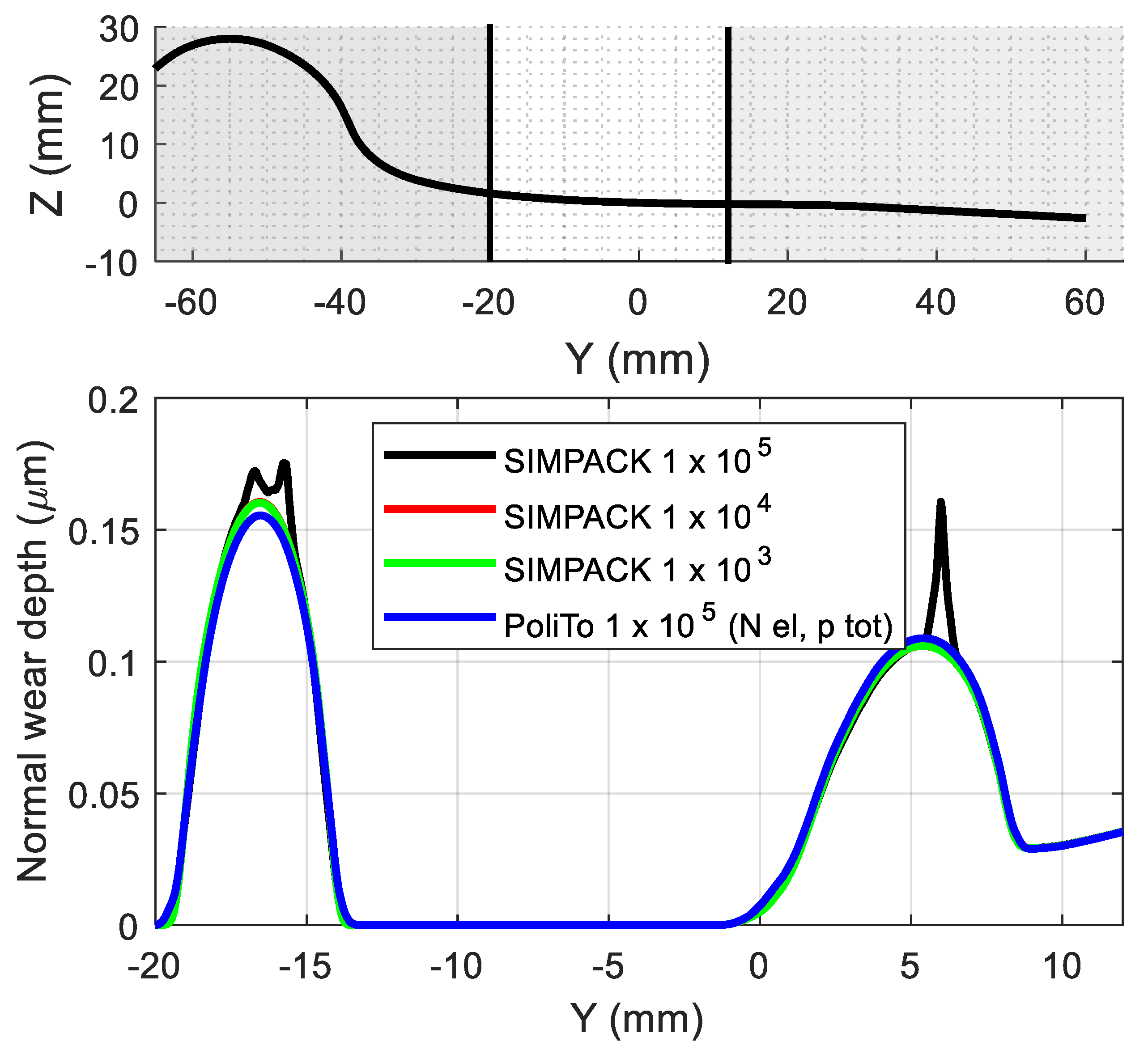
• With respect to Archard’s law, the KP law is less affected by changes in the contact reference damping applied to avoid numerical instabilities in the calculation of the wheel–rail contact forces. Nonetheless, a preliminary tuning of the reference damping should always be performed to ensure reliable results in terms of wear depth and worn profile shape. Conversely, the number of discretization elements on the contact patch has a negligible impact on the wear depth distribution, but it can threaten the convergence of the numerical integrator during the simulation, especially when using the EE method.
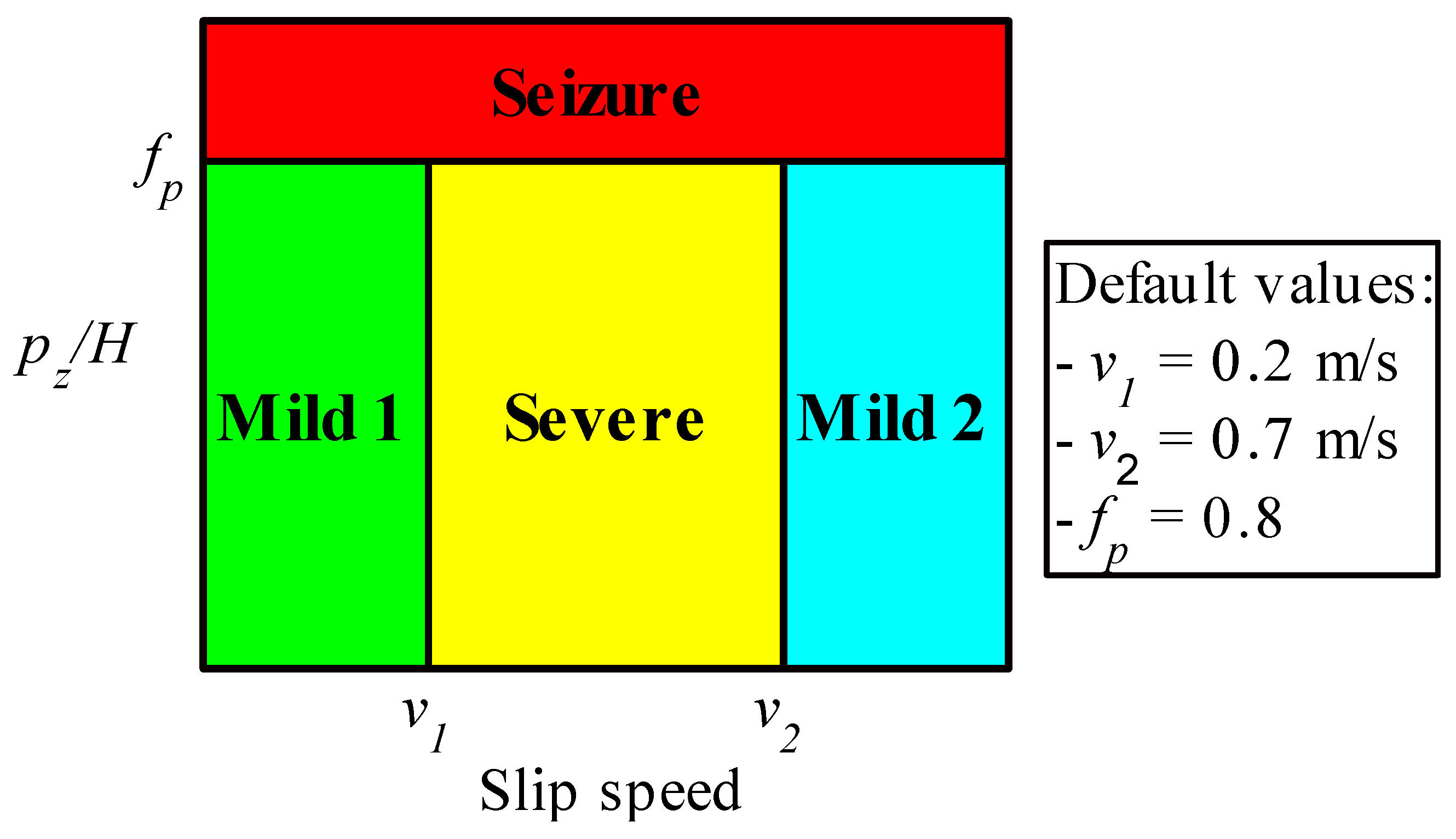
• For the KP law, the wear rate decreases with the curve radius, as all curves in the wear regime are severe in the simulations shown in the paper. On the other hand, Archard’s law does not feature a monotonous dependency of wear rate on curve radius because wider curves can be run at a higher speed, shifting from the mild 1 region to the severe region of the KTH wear map.
• Although the outcomes of the present paper suggest that the energetic KP law ensures more stability in the simulation and less dependency on modelling parameters, it is a less solid law in the literature, with many uncertainties on the wear coefficients and transition between the mild and severe regimes.
• The EE method, which considers an equivalent elliptic patch, provides wear depth distributions in good agreement with the outputs of the DE method, which considers a non-elliptic patch shape for the calculation of the tangential forces and wear depth. As the discrepancies between the two methods can be considered lower than the uncertainties related to the choice of the wear coefficients, and since the computational time can increase by one order of magnitude when shifting from the EE to the DE method, the EE method is believed to be the proper approach for the sake of the numerical simulation of the evolution of railway wheel profile shapes.
• It is demonstrated that the SIMPACK algorithm calculates the contact pressure using the total normal force, which is the sum of the elastic term and a damping term. Nonetheless, the simulations shown in the paper highlight that this strategy can produce local wear peaks when using Archard’s law, which states that worn volume is directly proportional to the normal force. These peaks arise when the number of contact patches has an abrupt change, and a new contact patch is generated with a small area, and with a normal force corresponding to the damping contribution only. This leads to large values of contact pressure corresponding to the seizure regime according to the KTH map. To avoid these peaks generated from numerical issues, the present paper suggests calculating the worn volume with the elastic component only, which acts as a sort of filtered normal force.
• Nowadays, the most suitable solution for wear prediction is to rely on the commercial code for the dynamic simulation, whilst developing an external routine to calculate the worn material and worn profile shape. With this strategy, it is possible to avoid numerical peaks more easily, to define track-variable wear coefficients (to consider for instance lubrication) and in general to gain further control of the wear computation with no loss of the unbeatable reliability provided by commercial codes for the dynamic simulation.

Future developments of the activities are intended to address the issues listed below:

• To run iterative wear simulations, with subsequent replacement of the wheel worn profiles, it is essential to adopt a suitable smoothing technique that avoids numerical instabilities whilst not compromising the worn shape of the profile. Consequently, different smoothing and filtering techniques should be tested to find the optimal strategy.
• Experimental activities on dedicated test rigs are planned to tune and validate the wear algorithms for the selected wheel and rail steel materials considering the variation in wear coefficients due to the possible influence of third-body materials at the wheel–rail interface such as lubricants or natural contaminants.

References

1. Enblom, R. Deterioration mechanisms in the wheel–rail interface with focus on wear prediction: A literature review. Veh. Syst. Dyn. 2009, 47, 661–700. [Google Scholar] [CrossRef]
2. Braghin, F.; Bruni, S.; Lewis, R. Railway wheel wear. In Wheel–Rail Interface Handbook; Lewis, R., Olofsson, U., Eds.; Woodhead Publishing: Cambridge, UK, 2009; pp. 172–210. [Google Scholar]
3. Pombo, J.; Desprets, H.; Verardi, R.; Ambrósio, J.; Pereira, M.; Ariaudo, C.; Kuka, N. Wheel wear evolution and its influence on the dynamic behaviour of railway vehicles. In Proceedings of the 7th EUROMECH Solid Mechanics Conference, Lisbon, Portugal, 9–11 September 2009. [Google Scholar]
4. Pombo, J. Application of a Computational Tool to Study the Influence of Worn Wheels on Railway Vehicle Dynamics. J. Softw. Eng. Appl. 2012, 5, 51–61. [Google Scholar] [CrossRef]
5. Pradhan, S.; Samantaray, A.K.; Bhattacharyya, R. Prediction of railway wheel wear and its influence on the vehicle dynamics in a specific operating sector of Indian railways network. Wear 2018, 406–407, 92–104. [Google Scholar] [CrossRef]
6. Pradhan, S.; Samantaray, A.K. A Recursive Wheel Wear and Vehicle Dynamic Performance Evolution Computational Model for Rail Vehicles with Tread Brakes. Vehicles 2019, 1, 88–115. [Google Scholar] [CrossRef]
7. H-Nia, S.; Flodin, J.; Casanueva, C.; Asplund, M.; Stichel, S. Predictive maintenance in railway systems: MBS-based wheel and rail life prediction exemplified for the Swedish Iron-Ore line. Veh. Syst. Dyn. 2024, 61, 3–20. [Google Scholar] [CrossRef]
8. Ye, Y.; Sun, Y.; Dongfang, S.; Shi, D.; Hecht, M. Optimizing wheel profiles and suspensions for railway vehicles operating on specific lines to reduce wheel wear: A case study. Multibody Syst. Dyn. 2021, 51, 91–122. [Google Scholar] [CrossRef]
9. Pires, A.C.; Pacheco, L.A.; Dalvi, I.L.; Endlich, C.S.; Queiroz, J.C.; Antoniolli, F.A.; Santos, G.F.M. The effect of railway wheel wear on reprofiling and service life. Wear 2021, 477. [Google Scholar] [CrossRef]
10. EN 14363:2016; Railway Applications—Testing and Simulation for the Acceptance of Running Characteristics of Railway Vehicles—Running Behaviour and Stationary Tests. CEN: Brussels, Belgium, 2016.
11. Pombo, J.; Ambrósio, J.; Pereira, M.; Lewis, R.; Dwyer-Joyce, R.; Ariaudo, C.; Kuka, N. A study on wear evaluation of railway wheels based on multibody dynamics and wear computation. Multibody Syst. Dyn. 2010, 24, 347–366. [Google Scholar] [CrossRef]
12. Pombo, J.; Ambrósio, J.; Pereira, M.; Lewis, R.; Dwyer-Joyce, R.; Ariaudo, C.; Kuka, N. A railway wheel wear prediction tool based on a multibody software. J. Theor. Appl. Mech. 2010, 48, 751–770. [Google Scholar]
13. Pombo, J.; Ambrósio, J.; Pereira, M.; Lewis, R.; Dwyer-Joyce, R.; Ariaudo, C.; Kuka, N. Development of a wear prediction tool for steel railway wheels using three alternative wear functions. Wear 2011, 271, 238–245. [Google Scholar] [CrossRef]
14. Enblom, R.; Stichel, S. Industrial implementation of novel procedures for the prediction of railway wheel surface deterioration. Wear 2011, 271, 203–209. [Google Scholar] [CrossRef]
15. Bosso, N.; Magelli, M.; Zampieri, N. Simulation of wheel and rail profile wear: A review of numerical models. Railw. Eng. Sci. 2022, 30, 403–436. [Google Scholar] [CrossRef]
16. Braghin, F.; Lewis, R.; Dwyer-Joyce, R.S.; Bruni, S. A mathematical model to predict railway wheel profile evolution due to wear. Wear 2006, 261, 1253–1264. [Google Scholar] [CrossRef]
17. Jin, X.; Xiao, X.; Wen, Z.; Guo, J.; Zhu, M. An investigation into the effect of train curving on wear and contact stresses of wheel and rail. Tribol. Int. 2009, 42, 475–490. [Google Scholar] [CrossRef]
18. Tao, G.; Ren, D.; Wang, L.; Wen, Z.; Jin, X. Online prediction model for wheel wear considering track flexibility. Multibody Syst. Dyn. 2018, 44, 313–334. [Google Scholar] [CrossRef]
19. Bosso, N.; Zampieri, N. Numerical stability of co-simulation approaches to evaluate wheel profile evolution due to wear. Int. J. Rail Transp. 2020, 8, 159–179. [Google Scholar] [CrossRef]
20. About Simpack 2023.4-Build150, 64bit; Dassault Systems Simulia Corp.: Santa Clara, CA, USA, 2023.
21. Krause, H.; Poll, G. Wear of wheel-rail surfaces. Wear 1986, 113, 103–122. [Google Scholar] [CrossRef]
22. Archard, J.F. Contact and Rubbing of Flat Surfaces. J. Appl. Phys. 1953, 24, 981–988. [Google Scholar] [CrossRef]
23. Archard, J.F.; Hirst, W.; Allibone, T.E. The wear of metals under unlubricated conditions. Proc. R. Soc. London. Ser. A Math. Phys. Sci. 1956, 236, 397–410. [Google Scholar] [CrossRef]
24. Jendel, T. Prediction of wheel profile wear—Comparisons with field measurements. Wear 2002, 253, 89–99. [Google Scholar] [CrossRef]
25. Kalker, J.J.; Chudzikiewicz, A. Calculation of the Evolution of the Form of a Railway Wheel Profile Through Wear. In Unilateral Problems in Structural Analysis IV, Proceedings of the Fourth Meeting on Unilateral Problems in Structural Analysis, Capri, Italy, 14–16 June 1989; Piero, G., Maceri, F., Eds.; Birkhäuser: Basel, Switzerland, 1991. [Google Scholar]
26. Jendel, T.; Berg, M. Prediction of Wheel Profile Wear. Veh. Syst. Dyn. 2002, 37, 502–513. [Google Scholar] [CrossRef]
27. Bosso, N.; Magelli, M.; Zampieri, N. Study on the Influence of the Modelling Strategy in the Calculation of the Worn Profile of Railway Wheels; WIT Press: Southampton, UK, 2022; pp. 65–76. [Google Scholar]
28. Ignesti, M.; Innocenti, A.; Marini, L.; Meli, E.; Rindi, A. Development of a model for the simultaneous analysis of wheel and rail wear in railway systems. Multibody Syst. Dyn. 2014, 31, 191–240. [Google Scholar] [CrossRef]
29. Kisilowski, J.; Kowalik, R. Method for Determining the Susceptibility of the Track. Appl. Sci. 2022, 12, 12534. [Google Scholar] [CrossRef]
30. Kalker, J.J. A Fast Algorithm for the Simplified Theory of Rolling Contact. Veh. Syst. Dyn. 1982, 11, 1–13. [Google Scholar] [CrossRef]
31. Ayasse, J.B.; Chollet, H. Determination of the wheel rail contact patch in semi-Hertzian conditions. Veh. Syst. Dyn. 2005, 43, 161–172. [Google Scholar] [CrossRef]
32. Quost, X.; Sebes, M.; Eddhahak, A.; Ayasse, J.-B.; Chollet, H.; Gautier, P.-E.; Thouverez, F. Assessment of a semi-Hertzian method for determination of wheel–rail contact patch. Veh. Syst. Dyn. 2006, 44, 789–814. [Google Scholar] [CrossRef]
33. Bezin, Y.; Pålsson, B.A. Multibody simulation benchmark for dynamic vehicle-track interaction in switches and crossings: Modelling description and simulation tasks. Veh. Syst. Dyn. 2023, 61, 644–659. [Google Scholar] [CrossRef]
Figure 1. Wear zones and regimes according to KTH wear map.
Machines 12 00644 g001
Figure 2. Reference track data: curvature with speed profile (upper plot) and superelevation (lower plot). Positive values of curvature and superelevation are used for right-handed curves, while negative values refer to left-handed curves.
Machines 12 00644 g002
Figure 3. Zoom on a worn zone of the profile (note that point O is the origin of the reference system on the original profile).
Machines 12 00644 g003
Figure 4. Effect of contact reference damping and wheel–rail contact method on wear depth distribution (Archard’s law).
Machines 12 00644 g004
Figure 5. Effect of contact reference damping and wheel–rail contact method on wear depth distribution (KP law).
Machines 12 00644 g005
Figure 6. Wear volume and regimes with Archard’s and KP laws on the reference track curves (negative radius values correspond to left-handed curves).
Machines 12 00644 g006
Figure 7. Effect of different values on total normal load and contact pressure for Archard’s law.
Machines 12 00644 g007
Figure 8. Wear peaks produced with Archard’s law (the lower plot shows a zoom of the white region of the upper plot).
Machines 12 00644 g008