Abstract
Unmanned Aerial Vehicles (UAVs), as widely used tools, can achieve better efficiency when integrated into a multi-UAV system than individual, dispersed units. Obstacle avoidance and formation control are fundamental requirements for such systems. The Boids algorithm, a biomimetic model suitable for swarming, serves as the foundation for this study. This paper proposes a novel integrated algorithm based on Boids that can be applied to multi-UAV systems for obstacle avoidance and formation control. The algorithm enables the multi-UAV system to automatically form formations, autonomously avoid obstacles, and recover formations rapidly. In this algorithm, each UAV functions as an agent within the system that is capable of independently collecting and sharing information. Each agent can make independent decisions to enter either the formation mode or the obstacle avoidance mode based on external environmental factors. The formation mode utilizes the virtual structure method to guide UAVs to their virtual formation positions. In the obstacle avoidance mode, the artificial potential field method is employed to ensure that each UAV maintains a safe distance from other UAVs that pose collision risks and various complex obstacles, regardless of their number. Simulation experiments were conducted on the Unity platform, varying the number of UAVs and the formation shapes. The results verified that the algorithm operates correctly, stably, and in a timely manner, demonstrating good performance.
1. Introduction
Unmanned Aerial Vehicles (UAVs), as widely used tools, can achieve energy efficiency [] through various strategies, including optimizing quadrotor control for field inspections [] and trajectory optimization []. when they collaborate in a group as a multi-UAV system (MUS). This collaboration also enables the completion of more complex tasks, such as large-scale search and rescue operations [] and inspections []. In these applications, safety is a primary concern []. Therefore, as an important means to ensure safety, obstacle avoidance technology is particularly critical. Several scholars have used path planning [,,,] to achieve effective obstacle avoidance []. Recent studies have demonstrated the feasibility of UAV operations in constrained environments, where advanced localization and mapping techniques have significantly enhanced robustness and safety. In addition, these missions may require UAV swarms to have formation capabilities to ensure efficient and coordinated mission execution. In multi-UAV systems, obstacle avoidance algorithms and formation control are not only fundamental for enabling UAV cooperation but are especially crucial in complex environments. Effective obstacle avoidance strategies can prevent collisions between UAVs, thereby enhancing the system’s robustness and stability.
There are various control strategies in the field of UAV formation control, including leader–follower models [,,], the virtual structure approach [], behavior-based methods [], and bio-inspired self-organizing algorithms []. Among these, the Boids algorithm is one such bio-inspired method. The Boids model is a biomimetic clustering algorithm inspired by the group behavior of birds, fish schools, and other organisms whose movements appear synchronized and coordinated, where individual agents can converge and move in the same direction without physically colliding. From a physical perspective, this can be viewed as a model of motion and perception, and thus the Boids model was developed to simulate group dynamics on computers. Since Craig W. Reynolds first introduced the Boids algorithm [], it has been continuously improved and applied in various fields. For instance, the Boids algorithm has been used to simulate flocking behavior in animals [] and fish schools []. Since its optimization, the Boids algorithm has found appropriate applications in different domains. For example, Yao [] used the Boids model to analyze swarm behavior from GPS data. Knievels applied virtual Boids clusters around vehicles to reduce the impact of target location uncertainty on target recognition []. Cao incorporated Boids into swarm control strategies []. Many studies have demonstrated that the Boids model is particularly well suited for clustering, making it a potential approach for multi-UAV systems or other collective systems.
Indeed, numerous scholars have researched and optimized the Boids model for UAV applications. As early as 2012 [], researchers applied the Boids algorithm to UAVs. For example, Weiqiang Jin combined Boids with deep reinforcement learning to significantly improve the efficiency and reliability of multi-UAV pursuit-evasion tasks []. Zeng used a combination of Multi-Agent Reinforcement Learning (MARL) and Boids modeling to train UAVs, with the results showing good swarm adaptability, particularly in terms of cohesion and separation between agents []. These studies prove that the Boids model is feasible and advantageous when applied to UAVs. Many scholars have also deployed the Boids algorithm in UAVs to validate its obstacle avoidance and clustering effectiveness [,]. However, these studies primarily focus on the team-based obstacle avoidance and clustering effects within the UAV swarm. Few studies emphasize the formation, maintenance, and recovery of UAV formations, as well as the avoidance of complex external obstacles using Boids-based methods, [], especially considering the dynamic environments UAVs frequently encounter.
To address the gap in existing research, particularly in the context of multi-UAV systems operating in three-dimensional spaces with complex obstacles, this paper proposes an integrated algorithm that builds upon the Boids model’s strengths. The algorithm coordinates UAVs to form and maintain formations, avoid obstacles, and rapidly recover formations after obstacle avoidance. It is based on a combination of Boids, the virtual structure method, and the artificial potential field method, enabling automatic formation, autonomous obstacle avoidance within and outside the team, and rapid formation recovery.
The contributions of this paper are as follows: 1. Boids Model Extension: The proposed algorithm extends the Boids model by not only enabling obstacle avoidance between UAVs but also addressing external obstacles. It preserves the Boids’ cohesion, alignment, and separation behaviors, ensuring that agents that temporarily leave the formation to avoid obstacles maintain proximity to the formation and continue in the same direction. This avoids excessive deviation from the formation during obstacle avoidance and facilitates fast formation recovery after avoiding obstacles. 2. Leaderless Algorithm: This algorithm adopts a leaderless approach, where each UAV functions as an identical agent in the multi-agent system. Based on its circumstances, each agent can independently choose whether to enter obstacle avoidance mode or maintain formation mode. Only the agents that need to avoid obstacles will perform obstacle avoidance, without affecting the behavior of other agents not in avoidance mode. This minimizes the impact of individual agents on the overall system, thus aiding in the rapid recovery of the formation. 3. Functionality and Performance: Functionally, the formation mode allows the multi-UAV system to form and maintain specified shapes. The obstacle avoidance mode can handle obstacles with complex boundaries and any number of obstacles. After avoiding obstacles, the system can recover the formation. In terms of performance, the algorithm improves the initial formation process and considers real-world scenarios where UAVs, due to inertia, cannot experience abrupt speed changes. To avoid frequent data jitter, linear interpolation is used to generate the next frame’s velocity based on the previous frame’s velocity, ensuring continuity.
This paper proposes an integrated formation and obstacle avoidance algorithm based on Boids for multi-UAV systems. The algorithm operates in a leaderless mode, where each UAV is treated as an equal agent within the system (subsequently referred to as “agent”). Each agent has both formation and obstacle avoidance modes and autonomously maintains the formation or performs obstacle avoidance based on its situation. After avoiding obstacles, the agent recovers its formation and moves toward the formation’s target point.
2. Model of Agent
2.1. Basic Model of Agent
This paper considers the MAS as a system composed of N points that work under the same space , in which each point has two attributes: velocity and position. i is the number of agents, i = 1, 2, …, N, which are denoted as and on the x-axis, y-axis, and z-axis, as shown in Equations (1) and (2). The vectors and follow vector operations:
2.2. Agent Information Model
Each agent scans the surrounding environment and stores the information in six different information tables. The information tables are mainly divided into synchronized and private information tables. There are three independent and private tables: the table of surrounding agent neighbors, the table of collision-risk agent neighbors, and the table of collision-risk obstacles, which are private to each agent and can only be accessed and modified by the agent that owns them. There are three synchronized information tables: the table storing the positions of all agents, the table storing the positions of obstacles, and the table storing the formation errors of all agents.
Each agent is responsible for detecting obstacles within the range of its sensor and recording its own position and formation error. After detection, when an agent needs to modify the information in the public table, it broadcasts its updated information within a circular area of radius R. At the same time, the other agents within the circular area receive the information and change their own synchronized information table to achieve information synchronization. The other agents in the circular area receive the information and update their own synchronized information tables to achieve information synchronization.
2.3. Agent Judgment and Model Coordination
After gathering information, agents and obstacles are categorized into different boundary ranges based on their distance, which determines their influence, as shown in Figure 1.
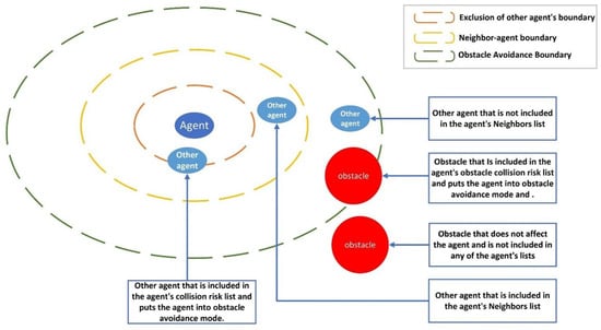
Figure 1.
Agent judgment of the effects of other agents and obstacles.
Each agent has boundaries to help assess its surroundings and make informed decisions about formation control and obstacle avoidance. The three types of boundaries and their effects when interacted with by other agents or obstacles are defined as follows:
- Neighbor–Agent Boundary: A predefined radius around a UAV that identifies other agents as “neighbors” if they enter this zone.
- Influence: UAVs within this boundary are added to the current agent’s neighbor list. The UAV adjusts its position to maintain coordination and formation while ensuring smooth movement without unnecessary evasive maneuvers.
- Exclusion Boundary for Other Agents: This boundary defines the range within which other UAVs or obstacles are considered potential collision threats.
- Influence: If an agent or obstacle enters this boundary, it is added to the collision risk list. The UAV then initiates avoidance maneuvers, such as adjusting its flight path or speed, to prevent collisions.
- Obstacle Avoidance Boundary: A specific boundary used solely for detecting obstacles rather than other UAVs.
- Influence: If an obstacle enters this boundary, the UAV switches to an avoidance mode and considers the obstacle a collision risk. Unlike other agents, obstacles do not participate in formation coordination, meaning the UAV prioritizes avoiding them over maintaining formation.
As the agent moves toward the target point, it encounters external obstacles and nearby agents while simultaneously maintaining formation and reaching the target. In response to these conditions, the agent switches between formation and obstacle avoidance modes as needed. The overall process is shown in Figure 2.
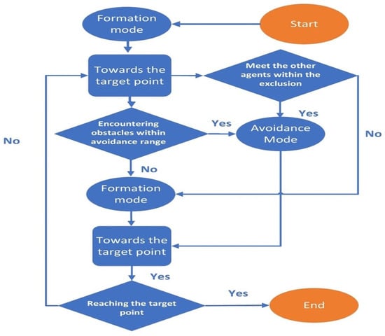
Figure 2.
Overall process of mode switching by the agent.
The partial pseudo-code for model selection is shown in Algorithm 1.
| Algorithm 1 Model selection |
| Require: Current agent instance b, list of all agents B, list of obstacles O Ensure: Updated velocity and position for b
|
3. Formation Mode
The formation mode is used for the initial formation of the MAS, as well as for its maintenance and updates. The agent enters the formation mode after eliminating the risk of collision and exiting the obstacle avoidance mode. This allows the agent to focus on positioning itself accurately, ensuring a precise and stable formation.
3.1. Mathematical Model of Formations
This section outlines how to use the virtual structure method to control the formation of agents and the basic formation model. The basic idea of the virtual structure method is to regard the formation of multiple-agent systems as a virtual rigid structure, where each agent has a fixed position relative to the formation center. This is equivalent to establishing a stable local coordinate system based on the center of the formation. Compared with the pilotage method, the virtual structure method can incorporate the formation error of each agent as feedback to influence subsequent formation control, thereby improving overall formation control capability. In particular, if an agent cannot return to the formation for a long time due to certain factors, the remaining agents will not abandon it by simply following the navigator; instead, they will wait and attempt to maintain the formation through feedback regulation. This paper sets the center point of the model as , which is initialized by Equation (3). The spacing between agents in the ideal formation is D, and the ideal formation position of agent i is .
A local coordinate system is established, with as the origin, while the agent is aligned according to . The following are the mathematical models for linear, circular, and equilateral triangle formations, as shown by Equations (4)–(9), respectively.
(1) Linear formation:
(2) Circular formation:
is the sector angle. For the circular formation design in this paper, the angle is at least 20° to ensure formation performance. R is the ideal circular radius calculated from the angle and spacing through Equation (5), and Equation (6) yields .
(3) Triangle formation:
In this formation method, each agent determines its position based on its serial number (starting from 1). First, using Equation (7), the number of hierarchies for the formation, , is calculated through an iterative formula based on the agent’s maximum serial number. Then, using Equation (8), the specific hierarchy in which each agent is located is determined. Finally, using Equation (9), the serial number of the side of the triangle (where the three sides are numbered 0, 1, and 2) in which the agent is positioned, , is obtained.
In Equation (7), n is the number of iterations of , and n is increased by 1 for each iteration of the operation.
Agents with hierarchy numbers serve as the vertices of the triangle. Their positions are located at the three vertices of the triangle, denoted as , and their positions are calculated using Equations (9)–(12). The remaining agents are positioned on the edges of the triangle, with their ideal positions determined by Equation (13). Figure 3 illustrates a triangular formation.
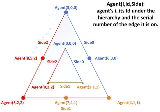
Figure 3.
Nine agents form a triangular formation with a hierarchy of 2. Each agent, based on its original i-number, is assigned the hierarchy to which it belongs and its ID within the hierarchy.
3.2. Fast Initial Formation Generation Strategy
The and position of each agent are randomized when generating the formation. The agent moves toward the target point (the mouse position on the Unity platform) while performing the formation. However, at initialization, the agent is farther away from the target point and relatively closer to the ideal formation position . In addition, the initial speed of each agent in the system is inconsistent at initialization.
In such a case, if this method is still used, the influence of the multi-agent system converging to the target point during initialization will be greater than the influence of formation, causing the agent to appear closer to the formation position but not accurately reach it due to excessively following the target point. This will affect the formation integrity of the entire system and prolong the formation time. At the same time, if the difference in initial speed between the agents is large, it will cause a significant gap between the agents as they converge to the target point. This not only prevents the formation from being completed but also causes the faster agents to reach the destination and then wait for the slower agents.
To solve this problem, this paper uses the method of a virtual target point during the formation generation period to assist with the formation and initialize the speed adjustment. At the start of the formation, a virtual target point moves in a circle around the system. Once the formation is established, this virtual point is replaced with the real formation target point. By generating a more uniform and stronger convergence velocity toward the target point, the speeds of all the agents converge in the same direction, completing the formation faster. At the same time, the virtual target point is positioned closer to the MAS for circular motion. For each agent with different , this allows adjustment during the process of following the virtual target point, ensuring rapid convergence and the maintenance of the formation after it is completed.
3.3. Formation Maintenance and Tendency
After each agent i obtains its respective , the agent calculates the distance from using Equation (14) and derives the temporary velocity based on using Equation (15). Meanwhile, to achieve the convergence of the entire agent formation toward the destination point , each agent derives the distance from using Equation (16). The final and of the considered destination are combined into Equation (17) to obtain a smoother, destination-oriented new velocity , which helps the agent converge to quickly while maintaining the formation.
In Equation (15), is the weighted value of .
In Equation (17), is the weight of , and is the weight of .
3.4. Formation Feedback Control
The virtual center point motion is adjusted through the feedback of each agent so that the final formation depends on the motion status of each agent, thus strengthening the overall control of the formation and improving its robustness. denotes the distance under a certain frame, which is a parameter that varies with time. The distance of each agent is processed through the weight coefficient to affect the velocity at the center of the virtual structure through Equation (18), and the new center point velocity is derived.
In Equation (18), is the weighted value of .
4. Barrier Avoidance Mode
The obstacle avoidance model of this algorithm is based on Boids, extended to achieve collision avoidance and clustering during obstacle avoidance. Boids [] is a model that simulates the behavior of biological clusters. It is also the earliest agent-based model with social characteristics and follows three basic rules: separation, alignment, and cohesion. These rules ensure that individuals gather as much as possible to form a group while avoiding being too close to nearby agents to prevent collisions. Additionally, the speed and direction of the agents and the group remain synchronized. The cohesive centripetal and isotropic rules of the obstacle avoidance model enable agents that are separated from the group due to obstacle avoidance to move closer to the formation. This is complemented by the fact that agents who have finished obstacle avoidance enter the formation mode to restore the formation.
4.1. Obstacle Avoidance Based on Artificial Potential Fields with Boids Rules
However, Boids themselves do not have obstacle avoidance. So, the present algorithm, based on the Boids algorithm, includes an obstacle collision risk list for dealing with obstacles in addition to the neighbors list that satisfies the cohesion rule. This collision risk list prevents collisions between agents, as previously mentioned. The algorithm uses the artificial potential field method to implement the three rules of Boids and handle external obstacle avoidance.
A single agent is regarded as a point, and a circular area is delineated as the required obstacle avoidance range by taking this point as the center and using the set obstacle collision risk distance R as the radius. When an obstacle enters this safety range, the agent disengages from the formation mode and enters the obstacle avoidance mode. The agent then uses the Boids-based obstacle avoidance algorithm, which first obtains the position of each obstacle, labeled as . Here, i represents the serial number of the obstacle in this agent’s obstacle table at this moment. The average position of N obstacles, , recorded in the obstacle table is derived from Equation (19). Meanwhile, the spacing between and the position of the agent is given by Equation (20).
To achieve obstacle avoidance, an agent backs away from the obstacle. The artificial potential field method is used here by calling a negative coefficient in the global variable of BoidsSpawner with to derive the artificial potential field force through Equation (21).
From the above equation, the closer the agent and the obstacle are, the smaller is, so the larger the absolute value of as a coefficient becomes, the larger the role of the artificial potential field increases. On the other hand, if the distance increases, the effect of decreases. is multiplied by the negative correlation coefficient so that moves in the direction of the negative gradient. Then, , in turn, generates this agent’s . This force is determined by combining the old velocity with Equation (22), which serves as a factor generated in case of obstacle avoidance by this agent. As a result, its effect is to make the agent tend to turn away from the direction of the obstacle, thus increasing the distance between the agent and the obstacle. This distance continues to grow until exceeds R, taking the agent out of the danger range and achieving obstacle avoidance.
Its effect is to make the agent turn away from the direction of the obstacle. As a result, the distance between the agent and the obstacle increases until it exceeds R and moves out of the danger range, achieving obstacle avoidance.
The purpose of the separation of Boids is to make the agent turn away from other risky agents in the surroundings. Similarly, the obstacle avoidance of Boids adopts the negative artificial potential field. The difference is that the range of collision risk of the agent and the correlation coefficient of the call are smaller than those of the obstacle avoidance, taking into account the fact that the agents are still clustered within a certain range. In addition, the location information of neighboring agents within the collision risk range is collected by the agent in the collision risk list, and finally, the factor is generated to affect the new speed.
The cohesion and alignment rules of Boids, on the other hand, use the positive artificial potential field, which is opposite to repulsion and obstacle avoidance. Specifically, the correlation coefficients and are positive, causing to move along the positive gradient direction. The purpose is to make each agent move toward the average position and average speed of its neighboring agents. The resulting factors influencing the agents are and .
Considering that the three rules of obstacle avoidance affect the agent differently, the values of the correlation coefficients vary. This algorithm prioritizes ensuring that the agent does not collide, and the correlation coefficients are as follows:
Table 1 shows the parameter weight configuration of Boids in common cases, where is larger than and much larger than the remaining two attributes. This ensures that the individual agent prioritizes avoiding obstacles and collisions with neighboring agents. This parameter configuration is also used in the experiments presented in this paper.

Table 1.
List of weighting parameters.
4.2. Obstacle Avoidance Speed Update Based on Linear Interpolation Method
When agent obstacle avoidance is considered, the simultaneous application of the three Boids rules and obstacle avoidance can cause discontinuous changes in the agent’s velocity. This results in unreasonable and sudden changes in speed, as well as frequent data jitter, due to the conflicting influences of the positive and negative artificial potential fields. To address this issue, the linear interpolation method is used to calculate the new speed for the next frame, based on the original speed, as described in Equation (23).
In Equation (23), is a parameter that adjusts the generated factors by considering obstacle avoidance, the rules of Boids, and the old velocity.
The advantage of this algorithm is that the new speed is not directly synthesized from the factors of obstacle avoidance and Boids rules alone. Instead, it is based partly on the old speed and adjusted under the priority condition of ensuring safety, which makes the change in speed smoother and more reasonable.
5. Experimental Results
5.1. The Simulation Environment
In reality, there is a delay in the response of multi-agent systems, and they may also be subjected to network attacks that affect their nodes, leading to issues such as connectivity loss or Zeno behavior. Therefore, to simplify the experiments, this paper assumed smooth communication between multiple agents, with minimal to no delay in communication and free from attacks and other interferences, except for obstacles. In this paper, a simulation environment with complex obstacles was created using Unity(version 2022.3.0), with the Unity platform serving as the development environment. The unit of time was measured in frames, with a time interval of one frame. The length unit was Unity’s default unit (unit).
In these experiments, the number of iterations (frames) was used to measure the efficiency of the algorithm, while the distances between agents and between agents and obstacles were used to evaluate the effectiveness of obstacle avoidance. Among these, the number of iterations and the distances between agents and obstacles were the key metrics, and these metrics were used as reference benchmarks in the experiments in this paper.
5.2. Formation Generation Experiment and Analysis
The formation of the MAS in this experiment consisted of nine agents. In the beginning, the agents were randomly distributed in three-dimensional space. The experiment was considered successful when the error range between the location of all agents and the ideal location of the formation was within 1 unit. Three types of formations were tested: straight line, circular, and equilateral triangle formations. The formation processes are shown in Figure 4, Figure 5, and Figure 6, respectively. Each figure presents the MAS formations at four time nodes: at the beginning, at one-third of the formation time, at two-thirds of the formation time, and at the time of formation completion.
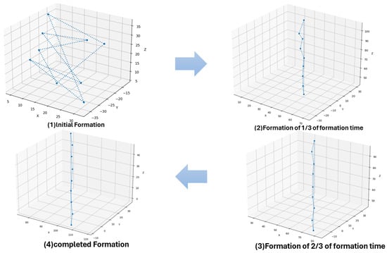
Figure 4.
Generation process of linear formation.
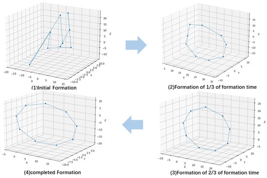
Figure 5.
Generation process of circular formation.
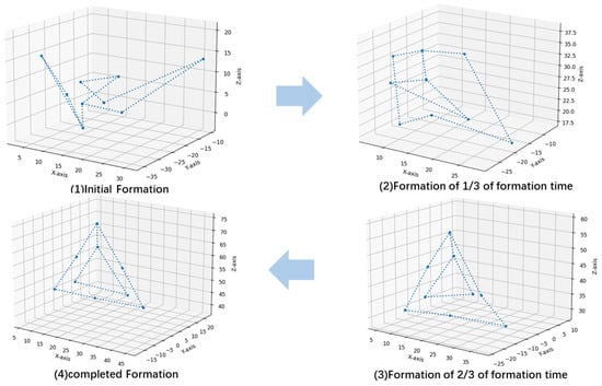
Figure 6.
Generation process of triangular formation.
In Figure 4, Figure 5, and Figure 6, it can be observed that the linear and circular formations reached the general outline of the formation faster (within one-third of the formation time) compared to the triangle formation, which mainly made smaller positional adjustments during the remaining two-thirds of the time.
The linear, circular, and triangular formations were tested, with the number of agents as a variable ranging from 3 to 18. The number of frames required for these formations is shown in Figure 7. According to Figure 7, the algorithm performed best with the linear formation, as the number of frames required was generally smaller than for the circular formation and much lower than for the triangular formation. Additionally, the number of frames required for both the linear and triangular formations increased with the number of agents, but the increase was relatively small, mostly staying below 1000 frames. The triangular formation exhibited more variation when the number of agents exactly matched the number required for each complete triangular layer, e.g., 3 (the number of triangles required for the first layer), 9 (3 + 6, the number of triangles required for two layers), and 18 (3 + 6 + 9, the number of triangles required for three layers). The number of frames required increased or decreased slightly, but when the number of agents did not meet the requirements of the hierarchy, the number of frames required for the formation increased sharply. Thus, triangular formations are sensitive to the number of agents, and adhering to the number of layers facilitates the formation process.
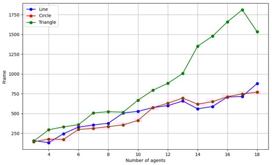
Figure 7.
Number of frames required for the three formations, depending on the number of agents.
However, it is also worth noting that, although the number of agents is theoretically unlimited, an increase in the number of agents requires more time for information exchange during execution. Additionally, running a large number of agents imposes high demands on the computational resources of the experimental computer. As a result, while the algorithm may be executable, severe time delays may prevent completion within a reasonable time, or the computer may become overloaded, leading to algorithm failure.
Finally, a comparative experiment was conducted to compare the algorithm with the formation control strategy based on the pilotage method, and the results are shown in Figure 8.
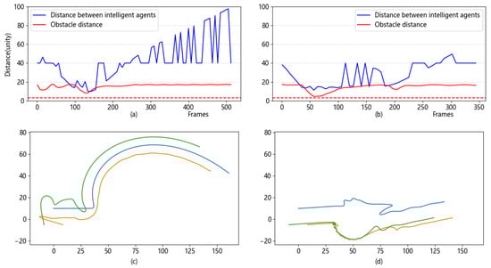
Figure 8.
Comparative experimental plots of the pilotage method and the algorithm. (a) Shortest distance over time for the pilotage method. (b) Shortest distance over time for the algorithm. (c) Trajectory of the pilotage method. (d) Trajectory of the algorithm.
When comparing subfigures (a) and (b) in Figure 8, it can be observed that, compared to the pilotage method, where the distance between agents was mostly within the range of 10–80 units, the present algorithm maintained the distance between agents mostly within the range of 20–40 units, This led to smaller fluctuations and better maintenance of the distance between agents. When comparing subfigures (c) and (d), it can be seen that, when facing the same obstacle, the algorithm caused the agents to spread out above and below the obstacle to avoid it, rather than adopting similar routes to pass above the obstacle en masse, as in the pilotage method. This shows the better flexibility of this algorithm in avoiding the obstacle.
5.3. Maintenance of Formation Experiments
In this experiment, a MAS with 10 agents was allowed to move in 3D space in linear, circular, and triangular formations along a figure-eight-shaped route, consisting of two circles with a radius of 65 units.
Figure 9 shows the continuous and complete trajectory diagram of each agent completing the figure-eight-shaped route. From this, it can be observed whether there was any deviation from the trajectory or if there was any trajectory jitter. As shown in Figure 9, every 60 frames, the location of each agent was intercepted. All location points at that time constitute the formation of the MAS, which provides a good response to the maintenance of the MAS formation, This helps determine whether the MAS undergoes deformation due to movement.
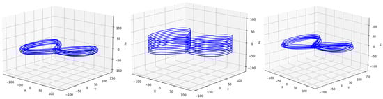
Figure 9.
From left to right: diagrams of the complete trajectories for the straight-line, circular, and triangular formations performing a figure-eight movement.
From the trajectory diagrams in Figure 9, it can be observed that each agent moved very smoothly along the predefined route without any jittering or deviation.
In Figure 10, it can be observed that the formations remained intact and the agents were not dispersed by movement.
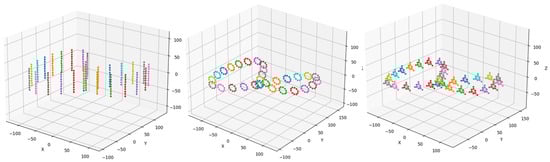
Figure 10.
From left to right: the formation changes of straight-line, circular, and triangular formations during a figure-eight movement are plotted.
Figure 11 illustrates the shortest distance between agents at the same time. It shows that there was a distance of 6.2 units between agents, indicating that the agents maintained a safe distance from each other without collisions while performing linear, circular, and triangular formations under this algorithm.
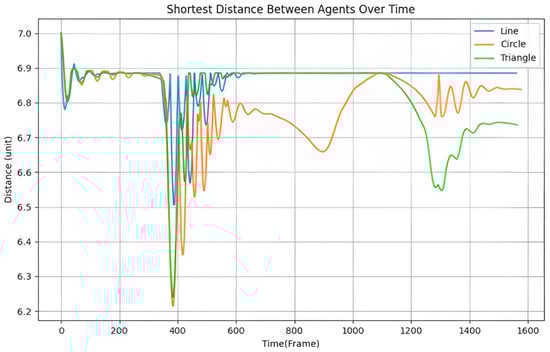
Figure 11.
The shortest distance between agents for the three formations when moving along the figure-eight-shaped route.
5.4. Obstacle Avoidance Experiments
In this experiment, the number of agents in the MAS was set to 10. Initially, the center of the MAS was located at the coordinates (0, 0, 0) from the x-, y-, and z-axes. The MAS maintained straight-line, circular, and triangular formations to advance along the positive x-axis in three trials, respectively. During the experiment, the MAS encountered an obstacle (its structure is shown in Figure 12), which had a complex boundary consisting of two rectangles with perpendicular cross-centers at (51, 0, 20). The obstacle measured 34 units along the x-axis, 50 units along the y-axis, and 4 units along the z-axis, resembling a cross. At this point, the MAS performed obstacle avoidance.
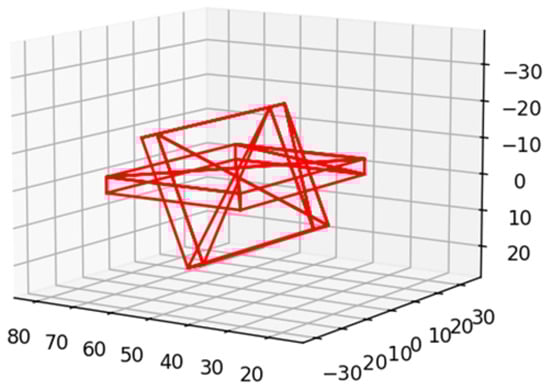
Figure 12.
The structure of the obstacle.
The complete trajectory of each agent in each of the three formations during this process was recorded and is shown in Figure 13.
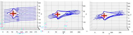
Figure 13.
From left to right: the continuous trajectory diagrams of three different formations during obstacle avoidance with one obstacle.
The trajectory diagrams in Figure 13 show that when encountering the obstacle, the agents chose to avoid it.
Multiple obstacles were also set up to conduct obstacle avoidance tests on the linear, circular, and triangular formations. The continuous trajectory diagrams for multiple obstacles are shown in Figure 14.
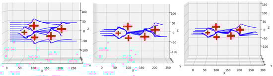
Figure 14.
The continuous trajectory diagrams of three different formations during obstacle avoidance with multiple obstacles.
The shortest distance between agents and obstacles in each formation was recorded while the MAS avoided multiple obstacles, as shown in Figure 15.
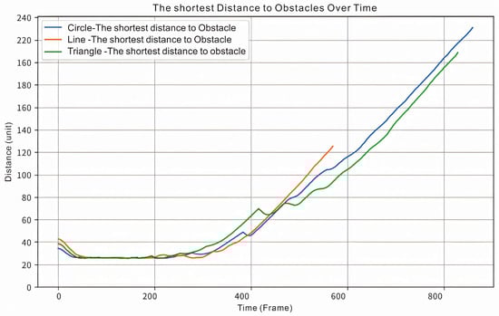
Figure 15.
The shortest distance between agents of three formations during obstacle avoidance.
Figure 15 illustrates that during obstacle avoidance, the agents maintained a distance greater than 0, indicating that the agents did not collide with each other. Together, Figure 13 and Figure 14 illustrate that even during complex obstacle avoidance, the agents of this algorithm successfully avoided both obstacles and collision with each other.
5.5. Resumption of Formation Experiments
In this experiment, the three MAS formations moved from the origin (0, 0, 0) to (500, 0, 0) and encountered the same cross-like obstacle as in Experiment 5.4, at the coordinates (50, 0, 0). The formation trajectories of the three formations were recorded when the obstacle was encountered, as shown in Figure 16.
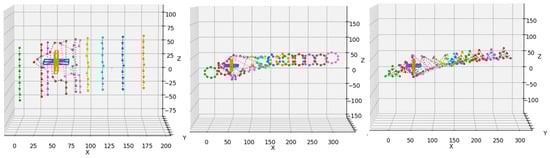
Figure 16.
The formation trajectories of three different formations for obstacle avoidance for one obstacle.
Figure 16 illustrates that when the agents of this algorithm encountered an obstacle, they momentarily broke away from their formation but then recovered the formation after passing the obstacle.
Next, the number of agents in the MAS was varied from 3 to 18 in the linear, circular, and triangular formations, and the same experiment as shown in Figure 15 was conducted 10 times for each configuration.
This experiment also recorded the number of frames taken from the last agent exiting the collision-risk zone of the obstacle to the moment when the MAS fully recovered its formation. This value represents the formation recovery time.
For each variable, the highest and lowest recovery time values were removed, and the remaining values were averaged. The final results are shown in Figure 17.
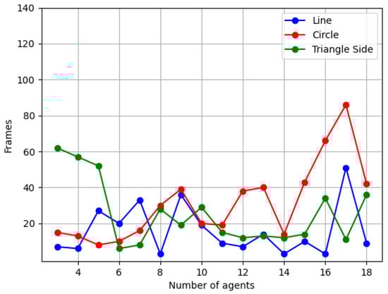
Figure 17.
The average number of frames taken by different numbers of agents in linear, circular, and triangular formations to recover after encountering an obstacle.
In Figure 17, the number of frames taken to recover the circular formation shows an increasing trend with the increase in the number of agents, while the number of frames taken to recover the linear and triangular formations correlates less with the number of agents, and the frame count is more random. However, the number of frames taken by these two formations is consistently lower than 65 fps, with most values concentrated in the 20 to 40 fps range.
Finally, the gap between the desired position and the ideal position during formation recovery after encountering an obstacle was recorded. Taking the linear formation of 10 agents as an example, Figure 18 shows the gap in recovery distance for the linear formation along X-, Y-, and Z-axes while recovering the formation after obstacle avoidance. Figure 19 shows the overall recovery gap.
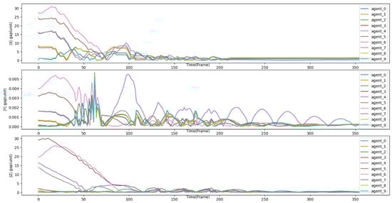
Figure 18.
The recovery gap in the X-, Y-, and -Z axes for a linear formation of 10 agents.
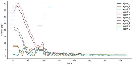
Figure 19.
The overall recovery gap for the linear formation of 10 agents.
5.6. Stability Experiments
The algorithm also demonstrated resistance to external disturbances. To test the immunity of the agents to disturbances of different strengths and frequencies, shifting crosswinds were simulated on the y-axis using Berlin noise.
Figure 20 shows that, during the first segment of the trajectory (green path), the agents under both wind disturbances initially maintained a relatively good formation. However, in the second segment (yellow path), as the wind effects accumulated, maintaining the formation became more challenging compared to the no-wind scenario. Significant deviations and fluctuations along the x-axis appeared. In the third segment (orange path), although deviations and fluctuations were still present, the agents started to recover, and the gap between their trajectories and the no-disturbance case began to narrow. In the final segment (blue path), the deviations and fluctuations almost disappeared, demonstrating the algorithm’s good recovery stability.
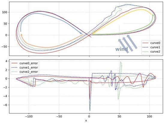
Figure 20.
The upper subfigure represents the motion trajectories of the agents, while the lower subfigure illustrates the variation of error values along the x-axis during the motion process. Curve 0 depicts the average motion trajectory of the linear formation composed of agents in the absence of wind disturbances. Curve 1 (with wind intensity of 1 f, wind turbulence of 0.3 f, and wind variation frequency of 0.7) and Curve 2 (with wind intensity of 2 f, wind turbulence of 0.5 f, and wind variation frequency of 1) represent the motion trajectories of the formation under different levels of wind disturbances.
6. Conclusions
This paper focuses on obstacle avoidance and formation control for multi-agent systems based on the Boids model. In the three-dimensional space, where the agents are randomly distributed, each agent determines whether to enter the formation mode or obstacle avoidance mode based on algorithms that consider safety boundaries and the distances between agents, obstacles, or other agents. In the formation mode, the virtual point method is used to quickly form the multi-agent system and coordinate the agents’ speeds to move toward the target point after completing the formation. In the obstacle avoidance mode, based on the Boids model, each agent follows Boids’ rules and functions while striving to maintain cohesion with the other agents and avoid collisions. The algorithm was tested in a simulation environment using the Unity platform, where the MAS successfully demonstrated both formation and obstacle avoidance. The test results show that the algorithm can form different shapes of formation without being constrained by the number of agents. The algorithm is particularly effective in circular and linear formations. In the obstacle avoidance test, the MAS under this algorithm could handle both simple and complex obstacle avoidance tasks and successfully recover after encountering obstacles.
In the future, the algorithm will be applied to a range of practical multi-robot systems, such as UAVs and detection carts. Consideration will be given to the practical needs of these systems, including the compatibility of mounted devices and addressing potential interference problems (e.g., noise environmental disturbances), to further enhance the algorithm’s performance.
Author Contributions
Data curation, J.Z. and J.N.; Writing—original draft, J.L., J.Z. and J.N.; Writing—review & editing, J.L.; Visualization, J.Z. and J.N.; Supervision, J.L.; Project administration, J.L.; Funding acquisition, J.L. All authors have read and agreed to the published version of the manuscript.
Funding
This research was funded by the Institute of Technology and Standards for the Intelligent Management of Air Navigation Safety, No. JG2022-18, and Research and development of a digital integrated operation system for the civil aviation pilot training system, 24CAFUC08003: Digital Operation Encore Solution and Demonstration Construction of Civil Aviation Pilot Training System with Chinese Characteristics No. MHAQ2024030.
Data Availability Statement
The raw data are publicly available. The data generated in Unity by the algorithm presented in this paper are available in the GitHub repository, accessed on 14 September 2024, at https://github.com/Claire-Zhao200/Data-for-Boids-based-integration-algorithm-for-formation-and-obstacle-avoidance-in-UAVs.git (accessed on 1 January 2020).
Conflicts of Interest
The authors declare that there are no conflicts of interest.
Abbreviations
The following abbreviations are used in this manuscript:
| UAVs | Unmanned Aerial Vehicles |
| MUS | Multi-UAV System |
References
- Nguyen, T.M.; Qiu, Z.; Nguyen, T.H.; Cao, M.; Xie, L. Persistently excited adaptive relative localization and time-varying formation of robot swarms. IEEE Trans. Robot. 2019, 36, 553–560. [Google Scholar] [CrossRef]
- Wang, Y.; Wang, Y.; Ren, B. Energy saving quadrotor control for field inspections. IEEE Trans. Syst. Man Cybern. Syst. 2020, 52, 1768–1777. [Google Scholar]
- Zeng, Y.; Zhang, R. Energy-efficient UAV communication with trajectory optimization. IEEE Trans. Wirel. Commun. 2017, 16, 3747–3760. [Google Scholar]
- Khan, A.; Gupta, S.; Gupta, S.K. Cooperative control between multi-UAVs for maximum coverage in disaster management: Review and proposed model. In Proceedings of the 2022 2nd International Conference on Computing and Information Technology (ICCIT), Tabuk, Saudi Arabia, 25–27 January 2022; pp. 271–277. [Google Scholar]
- Oh, K.K.; Park, M.C.; Ahn, H.S. A survey of multi-agent formation control. Automatica 2015, 53, 424–440. [Google Scholar] [CrossRef]
- Chaurasia, R.; Mohindru, V. Unmanned aerial vehicle (UAV): A comprehensive survey. In Unmanned Aerial Vehicles for Internet of Things (IoT) Concepts, Techniques, and Applications; John Wiley & Sons: Hoboken, NJ, USA, 2021; pp. 1–27. [Google Scholar]
- Debnath, D.; Vanegas, F.; Boiteau, S.; Gonzalez, F. An integrated geometric obstacle avoidance and genetic algorithm tsp model for uav path planning. Drones 2024, 8, 302. [Google Scholar] [CrossRef]
- Debnath, D.; Hawary, A.F.; Ramdan, M.I.; Alvarez, F.V.; Gonzalez, F. QuickNav: An effective collision avoidance and path-planning algorithm for UAS. Drones 2023, 7, 678. [Google Scholar] [CrossRef]
- Xu, H.; Niu, Z.; Jiang, B.; Zhang, Y.; Chen, S.; Li, Z.; Gao, M.; Zhu, M. ERRT-GA: Expert Genetic Algorithm with Rapidly Exploring Random Tree Initialization for Multi-UAV Path Planning. Drones 2024, 8, 367. [Google Scholar] [CrossRef]
- Shen, J.; Hong, T.S.; Fan, L.; Zhao, R.; Mohd Ariffin, M.K.A.b.; As’arry, A.b. Development of an Improved GWO Algorithm for Solving Optimal Paths in Complex Vertical Farms with Multi-Robot Multi-Tasking. Agriculture 2024, 14, 1372. [Google Scholar] [CrossRef]
- Wang, Y.; Lu, Q.; Ren, B. Wind turbine crack inspection using a quadrotor with image motion blur avoided. IEEE Robot. Autom. Lett. 2023, 8, 1069–1076. [Google Scholar] [CrossRef]
- Cowan, N.; Shakerina, O.; Vidal, R.; Sastry, S. Vision-based follow-the-leader. In Proceedings of the 2003 IEEE/RSJ International Conference on Intelligent Robots and Systems (IROS 2003) (Cat. No. 03CH37453), Las Vegas, NV, USA, 27–31 October 2003; Volume 2, pp. 1796–1801. [Google Scholar]
- Zhang, J.; Yan, J.; Zhang, P. Fixed-wing UAV formation control design with collision avoidance based on an improved artificial potential field. IEEE Access 2018, 6, 78342–78351. [Google Scholar] [CrossRef]
- Zhang, J.; Yan, J.; Zhang, P.; Kong, X. Collision avoidance in fixed-wing UAV formation flight based on a consensus control algorithm. IEEE Access 2018, 6, 43672–43682. [Google Scholar]
- Ren, W.; Beard, R.W. Decentralized scheme for spacecraft formation flying via the virtual structure approach. J. Guid. Control Dyn. 2004, 27, 73–82. [Google Scholar]
- Scharf, D.P.; Hadaegh, F.Y.; Ploen, S.R. A survey of spacecraft formation flying guidance and control (part 1): Guidance. In Proceedings of the 2003 American Control Conference, Denver, CO, USA, 4–6 June 2003; Volume 2, pp. 1733–1739. [Google Scholar]
- Wan, Y.; Tang, J.; Zhao, Z.; Chen, X.; Zhan, J. Systematic Review of Formation Control for Multiple Unmanned Aerial Vehicles. In Proceedings of the 2023 9th International Conference on Big Data and Information Analytics (BigDIA), Haikou, China, 15–17 December 2023; pp. 169–176. [Google Scholar]
- Reynolds, C.W. Flocks, herds and schools: A distributed behavioral model. In Proceedings of the 14th Annual Conference on Computer Graphics and Interactive Techniques, Anaheim, CA, USA, 27–31 July 1987; pp. 25–34. [Google Scholar]
- Lawrence, S.; Nehaniv, C.L. Aggregate boid behaviour to aid in artificial autopoietic organization. BioSystems 2024, 242, 105245. [Google Scholar]
- Niki, R.; Itami, S.; Fukuda, K.; Fukumi, J.; Sugino, R.; Yosimi, K.; Miyake, S. Development of Estimation Algorithm for Fish Schooling Pattern Using Boids Method. In Proceedings of the SICE Annual Conference 2023, Tsu, Japan, 6–9 September 2023. [Google Scholar]
- Yao, Y.T.; Hwang, R.H. Analysis of Swarm Behavior of Users’ GPS Data Based on Boids Model. In Proceedings of the 2014 IEEE International Conference on Internet of Things (iThings), and IEEE Green Computing and Communications (GreenCom) and IEEE Cyber, Physical and Social Computing (CPSCom), Taipei, Taiwan, 1–3 September 2014; pp. 421–427. [Google Scholar]
- Knievel, C.; Krueger, L. Sensor Object Plausibilization with Boids Flocking Algorithm. In Proceedings of the 2022 Sensor Data Fusion: Trends, Solutions, Applications (SDF), Bonn, Germany, 12–14 October 2022; pp. 1–5. [Google Scholar]
- Cao, H.; Chen, J.; Mao, Y.; Fang, H.; Liu, H. Formation control based on flocking algorithm in multi-agent system. In Proceedings of the 2010 8th World Congress on Intelligent Control and Automation, Jinan, China, 7–9 July 2010; pp. 2289–2294. [Google Scholar]
- Clark, J.B.; Jacques, D.R. Flight test results for UAVs using boid guidance algorithms. Procedia Comput. Sci. 2012, 8, 232–238. [Google Scholar] [CrossRef]
- Jin, W.; Tian, X.; Shi, B.; Zhao, B.; Duan, H.; Wu, H. Enhanced UAV Pursuit-Evasion Using Boids Modelling: A Synergistic Integration of Bird Swarm Intelligence and DRL. Comput. Mater. Contin. 2024, 80, 3523. [Google Scholar] [CrossRef]
- Zeng, Q.; Nait-Abdesselam, F. Multi-agent reinforcement learning-based extended boid modeling for drone swarms. In Proceedings of the ICC 2024-IEEE International Conference on Communications, Denver, CO, USA, 9–13 June 2024; pp. 1551–1556. [Google Scholar]
- Braga, R.G.; Da Silva, R.C.; Ramos, A.C.; Mora-Camino, F. Collision avoidance based on Reynolds rules: A case study using quadrotors. In Information Technology-New Generations: 14th International Conference on Information Technology; Springer: Cham, Switzerland, 2018; pp. 773–780. [Google Scholar]
- Vásárhelyi, G.; Virágh, C.; Somorjai, G.; Nepusz, T.; Eiben, A.E.; Vicsek, T. Optimized flocking of autonomous drones in confined environments. Sci. Robot. 2018, 3, eaat3536. [Google Scholar] [PubMed]
- Petrlík, M.; Báča, T.; Heřt, D.; Vrba, M.; Krajník, T.; Saska, M. A robust UAV system for operations in a constrained environment. IEEE Robot. Autom. Lett. 2020, 5, 2169–2176. [Google Scholar] [CrossRef]
Disclaimer/Publisher’s Note: The statements, opinions and data contained in all publications are solely those of the individual author(s) and contributor(s) and not of MDPI and/or the editor(s). MDPI and/or the editor(s) disclaim responsibility for any injury to people or property resulting from any ideas, methods, instructions or products referred to in the content. |
© 2025 by the authors. Licensee MDPI, Basel, Switzerland. This article is an open access article distributed under the terms and conditions of the Creative Commons Attribution (CC BY) license (https://creativecommons.org/licenses/by/4.0/).