Abstract
The rapid and accurate estimation of aboveground forest phytomass remains a challenging research task. In general, methods for estimating phytomass fall mainly into the category of field measurements performed by ground-based methods, but approaches based on remote sensing and ecological modelling have been increasingly applied. The aim is to develop the scientific and methodological framework for the remote sensing estimation of qualitative and quantitative characteristics of forest stands, using the combination of surveys and machine learning models to determine phytomass of forest stands and calculate the carbon balance. Even-aged stands of different tree species growing in the forest steppe zone of the East European Plain were chosen as test objects. We have applied the modernized methodological approaches to compare and integrate forest and tree stand characteristics obtained by ground-based and UAV-based comprehensive surveys; additionally, we developed computer vision models and methods for determining the same characteristics by remote sensing methods. The key advantage of the proposed methodology for remote monitoring and carbon balance control over existing analogues is the minimization of the amount of groundwork and, consequently, the reduction inlabor costs without loss of information quality. Reliable data on phytomass volumes will allow for operational control of the forest carbon storage, which is essential for decision-making processes. This is important for the environmental monitoring of forests and green spaces of various economic categories. The proposed methodology is necessary for the monitoring and control of ecological–climatic and anthropogenic–technogenic transformations in various landscapes. The development is useful for organizing the management of ecosystems, environmental protection, and managing the recreational and economic resources of landscapes with natural forests and forest plantations.
Keywords:
forest phytocoenoses; forest landscapes; canopy layer; morphometric parameters of trees; forest survey; phytomass; carbon stock; terrestrial environmental monitoring; remote sensing; vegetation indices; state of vegetation; landscape bioindication; synergy of methodological methods and approaches; machine/deep learning 1. Introduction
Global climate change has recently emerged as a serious long-term economic and environmental issue of universal concern [1,2]. Forest ecosystems play a significant role in the global carbon cycle; this has been confirmed by numerous scientific studies in recent decades [3,4,5,6].L. Chen et al. [7], C.I. Braga et al. [8], Y. Zhou et al. [9], A. Zielonka et al. [10], and other authors concluded that forest ecosystems contain approximately 80% of terrestrial carbon. It has been established that forest ecosystems play a significant role in reducing the concentration of greenhouse gases and mitigating global climate change [11,12,13,14,15,16,17].
Taking into account intensive forest management [18,19,20], deterioration of meteorological–climatic [21,22,23,24], and ecological [25,26,27,28,29] environmental parameters, the assessment of the bioproductivity of tree stands and forests [30,31,32,33,34] seems to be an urgent scientific and practical task. The long-term accumulation of stored carbon in forest ecosystems results in a biospheric effect related to the absorption of greenhouse gases, counteracting changes in the climate system of the planet [35,36]. Estimates of forest carbon stocks typically identify five primary pools: aboveground phytomass, belowground phytomass, deadwood (including standing and fallen dead wood), litter, and soil organic matter [3]. Aboveground phytomass is the key indicator of ecosystem productivity, forming qualitative and quantitative indicators of forest stands [37], as well as providingthe basis for the release of oxygen and carbon sinks [38]. Furthermore, determining the amount of carbon in soil and forest vegetation below ground is extremely difficult (and often impossible) when calculating plantation carbon stocks using remote sensing. The problem also lies in the obvious shortcomings of existing methods for the environmental monitoring of phytocoenoses through remote sensing.
The monitoring of the emissionand absorption of greenhouse gases by means of ground-based and remote sensing methods is extremely relevant and widely used in scientific and applied research [35]. Knowledge in the field of forest carbon accounting is currently increasing. However, different methodological approaches [38,39,40,41,42,43] and computational models [44,45,46,47,48] have been found to produce inconsistent results, highlighting the need for further methodological improvements.
This requires obtaining reliable information on the quantitative characteristics of forest stands and calculating the amounts of live and dead phytomass. Reliable estimation of phytomass in the context of climate change can provide a theoretical basis for the study of carbon cycling in terrestrial ecosystems [17,49], which has a crucial role in the response of forest ecosystems to greenhouse gas emissions [16,50]. The majority of authors [51,52,53] believe that a reliable assessment of aboveground forest phytomass will enhance the efficiency of management decisions in forest protection, conservation, and regeneration.
The most accurate method for estimating phytomass is in situ inventory with ground-based forest inventory methods [54]. The main disadvantage of the ground-based monitoring is high labor intensity, as this type of work involves a significant number of field surveys being conducted over an entire study area [55]. In addition, the problems with ground-based monitoring are related to the remoteness of the number of study sites from roads and settlements, the difficulty of moving across the study area, and often the inability to reach the forest area. This is especially true for the Central Forest Steppe zone of the East European Plain.
Rapid and accurate estimation of the aboveground forest phytomass remains a challenging research task [56,57]. In general, methods for estimating phytomass fall mainly into the category of field measurements made by ground-based methods, but remote sensing [58,59] and ecological modelling approaches have been increasingly applied [60,61].
It should be noted that remote sensing methods are of primary importance for over 70% of the Russian Federation's territory [62]. This is the optimal (and sometimes the only) method of obtaining statistically reliable and current information about forests for geographically remote and hard-to-reach areas [55].
Currently, satellite monitoring and assessment methods of forest states and structures are widespread in Russia and are used to estimate carbon balance [63,64]. With proper attribution of natural (disturbance) and anthropogenic (degradation) losses [65], the research has the potential to inform decision-making by governments across. It is well known that management and organizational decisions in relation to the rationalization of forest management, afforestation, the creation of plantings, and the environmental and economic control of plantings of different target categories are not sufficiently substantiated. This is observed in different administrative territories and geographical regions of the world. Focusing on research material on this issue is characterized by relevance and has practical benefits. Optical remote sensing images of Earth at various spatial, spectral, and temporal resolutions are freely available and are used to assess forest stands at various scales. This is reflected in the scientific works of many researchers [66,67,68,69]. Despite the obvious advantages of obtaining spatial data from satellite systems, this method of assessing forest stand phytomass has a significant disadvantage: the determination of forest tree stand characteristics is performed by analyzing the canopy of stands, but the resolution of satellite images does not provide detailed information. In addition, deadwood and understory vegetation are not taken into account. Assessments of carbon sequestration in the plantations often does not take into account the layering and structure of the forest stand. Carbon stock calculations are often very fragmented and based on approximate calculations.
Therefore, it is necessary for spatial data acquisition sources (camera type used, spatial resolution, survey age, etc.) to be enhanced. New methodologies and technologies need to be developed and implemented for the objective accounting of the carbon sink, allowing for the rapid estimation of phytomass in the forest stands, including the use of artificial intelligence (AI) [56]. Lidar technology based on the collection and analysis of data obtained using the laser scanning is widely used in the forestry sector [70]. Particularly, it can be successfully applied to improve our understanding of the three-dimensional structure of the forest environment [71]. It should be noted that there is practically lack of data on carbon sequestration in the lower layers of the forest phytocoenoses (including undergrowth and undergrowth) of the Central Forest Steppe of the East European Plain. In this regard, modern data are required on the state and productivity of forest ecosystems with differentiation according to different components of phytocoenoses.
Many researchers and scientists [72,73,74,75,76,77] have noted significant prospects for the automatic decoding of forest stands and analysis of forest ecosystems, including by laser scanning methods [78,79]. Specific vertical structuresare successfully recognized by the pattern of obtained dense point cloud and its shape using Lidars, including those based on UAVs [80]. In our study we used a combination of Lidar, RGB, and hyperspectral cameras. The effectiveness of the joint use of various types of sensors has been confirmed by many authors [81,82,83,84]. Their use corresponded to the purpose, theme, and problems of the work under consideration, as well as the idea of ensuring the synergy of advanced methodological approaches and technical means. This was necessary in accordance with the scientific idea and the specifics of our work.
Thus, the application of integrated ultra-high-resolution equipment during aerial survey [85,86] significantly increases informative and expands functional capabilities in phytomass assessment; it allows all silvicultural, bioecological, and tree stand characteristics to be identified, enabling us to determine carbon sinks in forests. Remote sensing is an extremely relevant and rapidly developing research area in the forestry industry. Remote sensing methods are widely in demand for use in assessing and monitoring forest stands.
The aim of the work is to develop the scientific and methodological basis for remote estimation of quantitative and qualitative characteristics of tree stands and ecosystems using colored light (RGB), Lidar, and hyperspectral surveys based on UAV and the presently widely accessible machine learning models (artificial intelligence)to determine aboveground phytomass of the forest stands and phytocoenoses.
Our proposed methodological approach for the remote ecological monitoring of the productivity of aboveground phytomass of forest ecosystems based on UAVs will provide more accurate and objective information about the state and structure of phytocoenoses. This methodological approach makes it possible to determine the carbon stock in natural forest stands and plantings and to carry out an accounting of forest resources. Our approach also allows us to monitor fire, environmental, and sanitary safety in forests.
2. Materials and Methods
2.1. Study Area
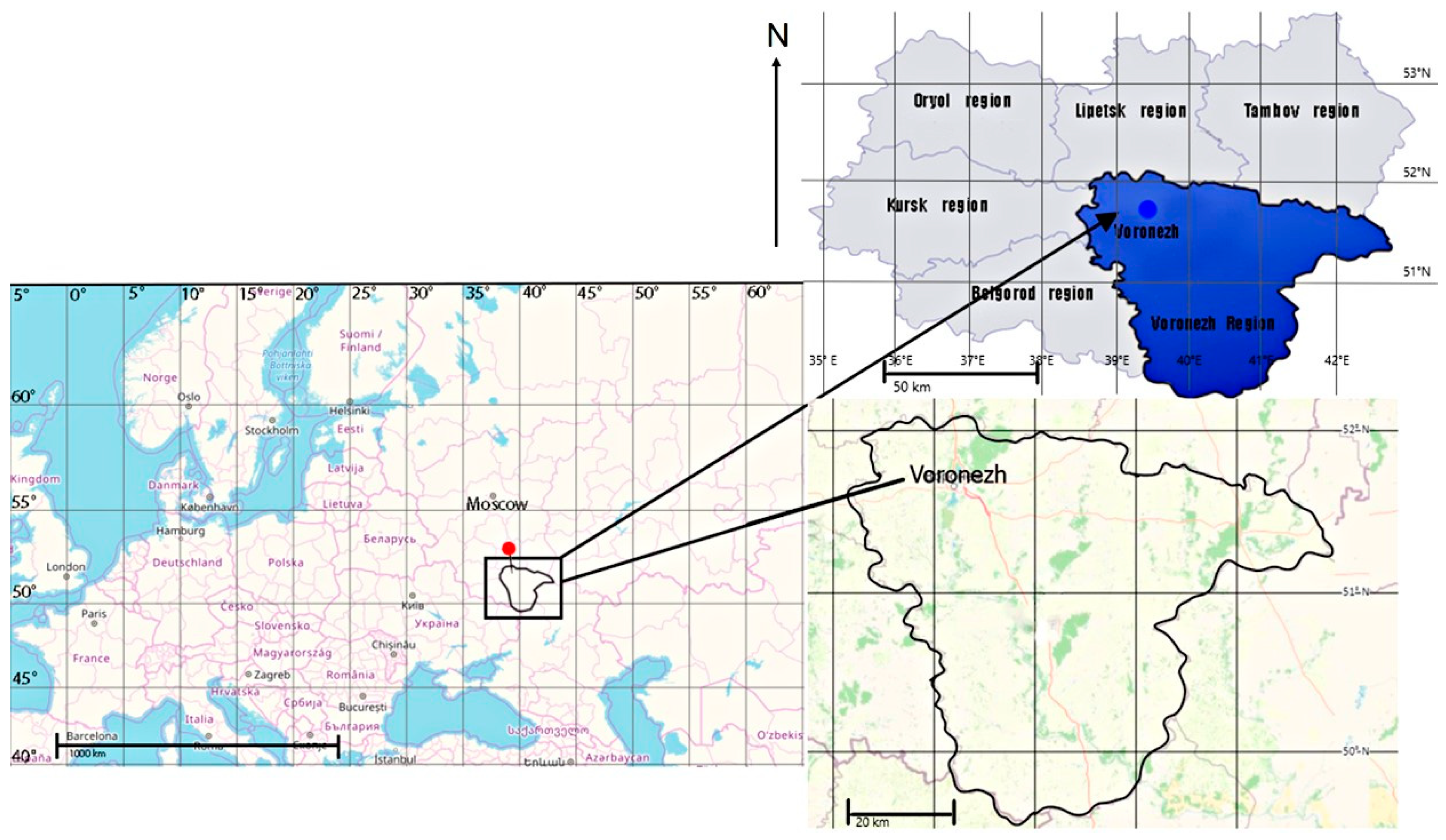
Considering the diversity of the forest vegetation in the Central Forest Steppe, this study assessed forest stands growing in the forest steppe zone using the example of the Suburban Forestry of the East European Plain (using the example of the Voronezh Region). The objects of the research were selected based on similar phytocoenotic, ecological, and physical–geographical conditions of the Central Forest Stepperegion. This ensured that the sample was representative and that reliable results were obtained for the general population. The location of the study sites is shown in Figure 1.
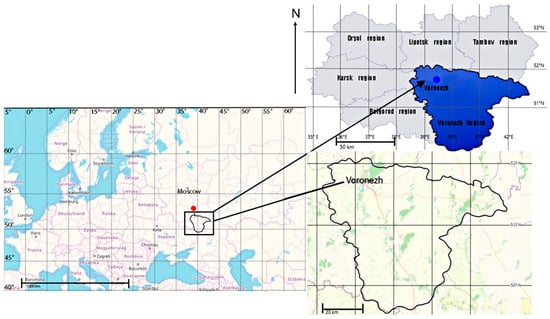
Figure 1.
Scheme of the study area location.
The research program included the following steps:
- Establishing sampling plots (Figure 2) in even-aged stands of different tree species composition and conducting the complete inventory on them with measurement of tree coordinates, species identification, trunk height and diameter, crown diameter, and tree state using ground-based inventory methods.
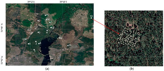 Figure 2. Location of trial plots on the territory of suburban forestry (numbers indicate the numberssampling plots): (a) sampling of the sites location; (b) placement of trees on SP 10.
 - Performing aerial surveys using the RGB, hyperspectral, and Lidar imagery from the UAVs to determine similar silvicultural and taxation characteristics using remote sensing methods.
- Generating training samples, designing computer vision models, and developing methods for determining the forest tree stand characteristics to calculate the phytomass of the forest stands using remote sensing methods.
- Comparing and integrating forest and taxation parameters of the stands obtained during ground-based inventories and parameters of the forest areas obtained using the RGB, hyperspectral, and UAV-based Lidar surveys.
- Application of the mathematical statistics and modelling methods to assess the accuracy of the results obtained, to verify the model validity, and to verify the developed algorithms.
- Development of the methodology for remote sensing of aboveground phytomass of forest stands for subsequent calculation of carbon stock in the forest area.
Fifteen sample plots (50 × 50 m) were established in the coniferous, deciduous, and mixed forest stands located in different forest growth conditions with moderately moist (fresh) types according to P.S. Pogrebnyak and in the different forest types according to V.N. Sukachev classification [87]. We studied even-aged (conditionally even-aged) stands growing in the following forest growth conditions: A2 (fresh pine forest), B2 (fresh pine–oak forest), C2 (fresh pine forest with birch, aspen, and oak participation), C2D (fresh pine forest with oak participation), D2 (fresh oak forest). The age of the forest stands was 80–100 years. The tree stand characteristics of the studied stands are shown in Table 1.

Table 1.
Species composition, tree stand characteristics, and forest growth conditions of the sample plots.
2.2. Ground-Based Forest Inventory
The full count was performed in all sample plots to determine tree species and the coordinates of individual trees, trunk diameter, tree height, crown diameter, and tree health state. Undergrowth, shrub layer, and the degree of coarse woody debris were identified and recorded.
The fieldwork was conducted utilizing modern geodetic and forest inventory equipment, including the SOUTH G2 GNSS receiver, Haglof Vertex Laser Geo altimeter. The methods employed were in accordance with the prevailing norms and legal frameworks in Russia [88,89,90].
Undergrowth and shrub layer were taken into account on the basis of the reforestation rules [91] and the forest management guidelines [92]. Undergrowth density degree (dense—over 8000 pcs. ha−1, medium—2–8000 pcs. ha−1, sparse—up to 2000 pcs. ha−1) and size categories (1—up to 0.5 m; 2—0.6–1.5 m; 3—over 1.5 m) were determined and species determination was performed. The shrub layer was estimated according to the following criteria: density degree (dense—more than 5000 pcs. ha−1, medium—2–5000 pcs. ha−1, sparse—less than 2000 pcs. ha−1), size (1—up to 1 m; 2—1–2 m; 3—more than 2 m), and species affiliation [90].
2.3. Estimation of the Aboveground Phytomass and Its Fractions
The estimation of aboveground phytomass stocks and its fractions (stem, branches, leaves) was conducted using allometric Equation (1) for each tree based on data on stem diameter at 1.3 m and tree height [93]:
where Pi—phytomass stocks and its fractions (i; stem with bark, branches, needles/leaves), kg dry weight; H—tree height, m; DBH—stem diameter at 1.3 m, cm; a0, a1 and a2—species-specific coefficients of allometric equation.
ln Pi = a0 + a1 ln H + a2 ln DBH,
To calculate the phytomass of pear (Pyrus communis L.), apple (Malus sylvestris L.), and mountain (Sorbus aucuparia L.) ash, the equation for bird cherry (Prunus padus L.) was used as the most closely related systematic category. The aboveground phytomass of undergrowth and shrubs with the DBH less than 8 cm was calculated for each species using their height according to allometric Equation (2) [94]:
where Pag—aboveground phytomass, kg dry weight; H—tree height, m; a and b—species-specific coefficients of allometric equation.
Pag = a × Hb,
Statistical analysis was performed using STATISTICA-13 [95]. Pearson correlation (3) and ANOVA analysis (4), as well as mathematical modelling techniques, were used [96].
The study employed regression analysis methods [97]. Parameter estimates for linear models, as well as those reduced to linear form, were calculated using least squares, and nonlinear least squares for all other cases. Student’s t-test was used to test the null hypothesis of statistical significance for the estimated parameter values. Grouped data (by sample area) were analyzed using both linear and nonlinear mixed-effects models. The accuracy of linear mixed-effects models was assessed by conditional and marginal coefficients of determination (R2) [98] (see Equation(5)). Pearson χ2-test of agreement [99] was used to determine the consistency between the results obtained from the machine learning models and the actual distribution series obtained during fieldwork (see Equation(6)).
The following criteria were used to assess the quality of the models:
Correlation coefficient:
Reliability of differences:
Coefficient of determination:
Pearson agreement criterion:
where M—mean value, m—standard error; xi, yi—actual value; ŷi—predicted value; ŷ—mean of actual values.
2.4. Flight and Survey Process
The data array was generated using the UAV payload (using combined equipment—RGB, Lidar, hyperspectral camera, and GNSS receiver). The Lidar and hyperspectral survey were performedfrom an unmanned aerial vehicle (UAV), Luftera LQ-5 (take-off weight 9.5 kg); digital photography in visible spectrum was performed from an unmanned aerial vehicle (UAV), Luftera LQ-4 (take-off weight 5.2 kg). The spatial resolution of the orthophotomaps was 2–2.5 cm/pixel.
The flights were performed at two altitudes, 60–70 m and 120–130 m, with horizontal speeds not exceeding 3 m/s and 6 m/s, respectively, to ensure sufficient overlap at the shooting interval of the 1 frame per second and to minimize blur. Hyperspectral imaging was performed using a Cubert S185 hyperspectral camera. Each frame taken by this camera is a combination of a panchromatic image in JPG format with a resolution of 1000 × 1000 pixels and a geometrically coinciding hyperspectral data cube of 50 × 50 = 2500 spectra. The spectral range is 450–950 nm; the number of spectral channels is 125.
2.5. Interpretation of the Tree Stand Characteristicsfrom High-Resolution Images
It should be noted that machine learning methods are not the primary focus of this paper. Moreover, the advances of machine learning methods have achieved such progress that they can be easily used in many practical problems. In this respect, the presented methods are well-known and universal, but require careful parameter tweaking for application for concrete forest plots.
For the neural network models, individual trees were labeled (tree species and its crown contour) on the small portion of each of the forest plots on the RGB geotiff-image. Data was prepared of the neural network classifier (bounding box rectangle were build)for each of the tree partitioning contours and data augmentation was applied for each of the images to improve robustness/generalizability. In particularsuch dataset was used to learn the model that was used to determine the tree species.
The neural network classifies the species of the individual trees. The condition and diameter of the crown were derived from this result. The computation of the hard-to-define taxation parameters was based on the identified relationships between the stand characteristics measured in the sample plots, the canopy digital model parameters, and the spectral characteristics of the aerial images. Training samples were generated from above mentioned labeled dataset and the YOLO neural network model was trained.
The characteristics of the forest stand were determined as follows:
- Tree canopy cover—by processing the RGB geotiffs;
- Tree height—by processing the Lidar imagery data;
- Precise tree location—by processing the Lidar imagery data;
- Tree species composition—from the RGB imagery using neural network models;
- Tree health state—with the hyperspectral data processing, based on the vegetation indices (NDVI, EVI, CVI);
- Crown diameter—using the RGB data processing and Lidar imagery;
- Stem diameter—by indirect indicators, based on the relationships identified using empirical relationships.
Traditional digital image processing techniques were used to separate trees from the background. The Lidar imagery uses geometric methods to interpolate the ground surface, namely by searching for the top of the forest canopy and then the height of the trees. Based on the Lidar imagery, the density of undergrowth and undergrowth in the stands was determined.
The complex of the calculation parameters includes the simplest indices NDVI, EVI, and CVI (Equations (7)–(9)), which allowed us to assess the condition of the tree stands (to identify the presence of dead or weakened trees).
where B—intensity of spectral radiation in the corresponding bands (µm); NIR—reflection in the near infrared region of the spectrum; RED—reflection in the red region of the spectrum; BLUE—reflection in the blue region of the spectrum; GREEN—reflection in the green region of the spectrum.
2.6. Remote Estimation of Aboveground Phytomass and Carbon Stocks
The main objective of the remote estimation methodology for aboveground phytomass and carbon stocks was to significantly minimize ground surveys. The methodology is based on a sequence of steps that include the implementation of automated methods for the remote estimation of vegetation using UAVs, based on the application of machine learning models (use of artificial intelligence).
- UAV-based determination using machine learning models:
- Study area’s coordinates, terrain features, and delineation boundaries for forest inventory;
- “Direct” silvicultural and stand characteristics, such as composition, height, crown diameter;
- Condition and degree of debris, especially deadwood, in the stands.
- Determination of “indirect” silvicultural stand characteristics such as age, stem diameter, canopy closure, and volume stock using reference materials and allometric equations, based on “direct” silvicultural and stand characteristics values.
- Determination of the density of the undergrowth and shrub layer based on UAVs using the Lidar transect developed by the authors, as well as calculation of the phytomass of subordinate layers based on the generated tabular model.
- Calculation of the carbon stock in the aboveground part of the forest stands (living and dead vegetation phytomass). Phytomass-to-carbon conversion factors were used according to IPCC guidelines [99]: 0.51 for coniferous tree species and 0.48 for broadleaved tree species.
3. Results
The methodological toolkit has been developed and a work algorithm has been defined that allows us to conduct remote assessment of the quantitative and qualitative forest characteristics with an accuracy that is comparable to that of traditional ground-based methods. The basis of the work algorithm is the integrated use of the Lidar, hyperspectral, and RGB survey materials using UAVs. This is necessary to obtain reliable information about the amount of aboveground phytomass and to calculate carbon reserves in the plantation by fraction. Information obtained online is extremely important for timely management decisions, for planning reforestation, and for environmental protection work.
3.1. Development of Technical and Methodological Tools for Determination of the Main Tree Stand Characteristics
3.1.1. State of Tree and Shrub Vegetation
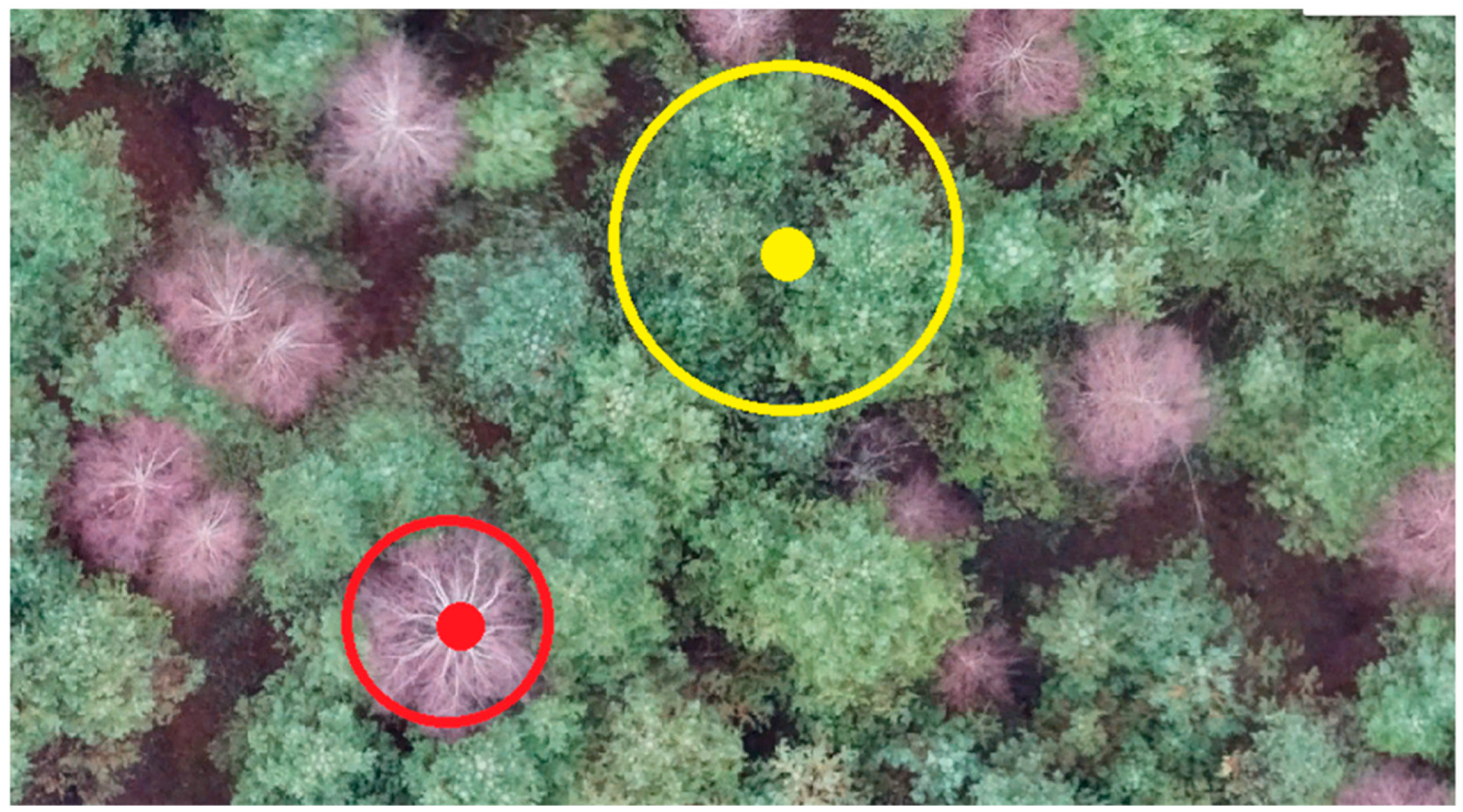
Determination of tree health category is based on vegetation indices calculation. The vegetation indices are constructed from hyperspectral data according to well-known formulas, based on the entire spectrum. Figure 3 shows selected areas in the forest area for the contrasting comparison and mapping of the proposed methodology. Dead trees are marked in red (NDVI-0.051), while fully viable trees are marked in yellow (NDVI-0.694).

Figure 3.
Selected areas for comparison of calculated indicators in the coniferous forest stands.
The point quantitative data of the vegetation indices reflecting the qualitative characteristic of the vegetation condition in the selected areas are collected in Table 2. Higher index values correspond to denser and greener vegetation in the analyzed fragment. The plots with dead trees have lower index values (NDVI less than 0.15). Vegetation indices are characterized by the greatest accumulation of chlorophyll in the plants. Therefore, the higher this value, the better the sanitary condition of the planting and the phytocenoses formed by them.

Table 2.
Calculation of some indices for selected areas.
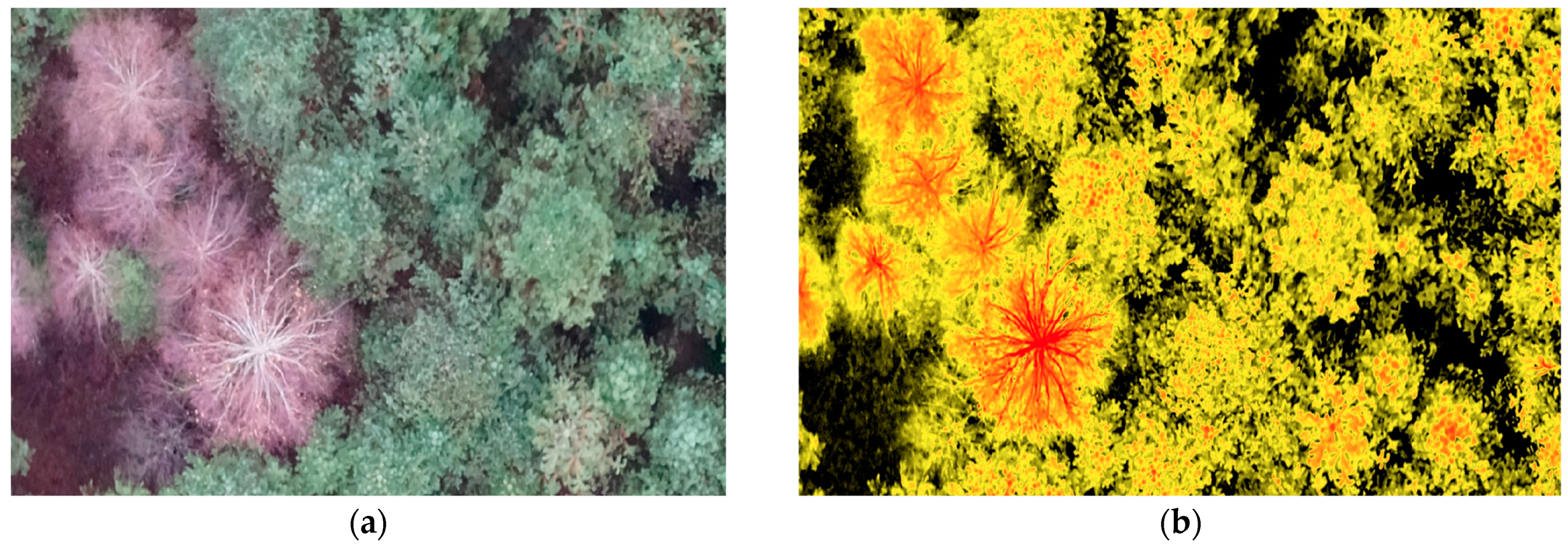
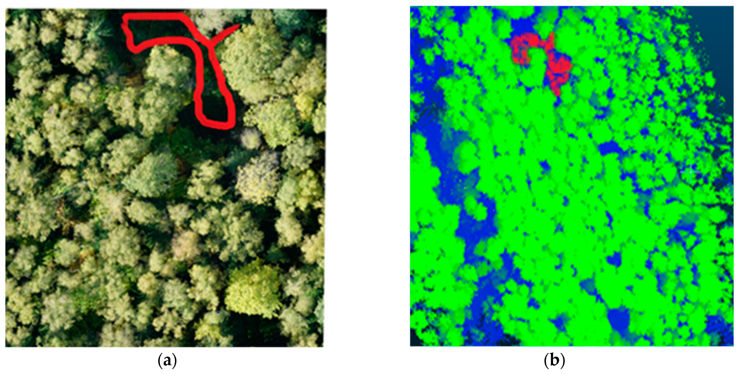
Figure 4 shows the forest plot with trees of different health categories. The calculated NDVI layer is superimposed on the original image, whereby the presence of dead and viable trees in the area can be identified: yellow (tree stand, understorey, shrub layer) reflects viable vegetation, black reflects dense ground cover, and red reflects the reduced NDVI value and allows for the identification of dead trees.

Figure 4.
Fragment of images of trees with dead/lost foliage and healthy trees: (a) RGB photo; (b) superimposed NDVI calculation layer.
3.1.2. Determining Tree Coordinates and Measurement of Stem Height and Crown Diameter
The initial task of remote sensing data analysis (RGB complex, Lidar, and hyperspectral imagery) is to determine the location (coordinates) of trees in order to determine the main taxonomic characteristics of the tree stand.
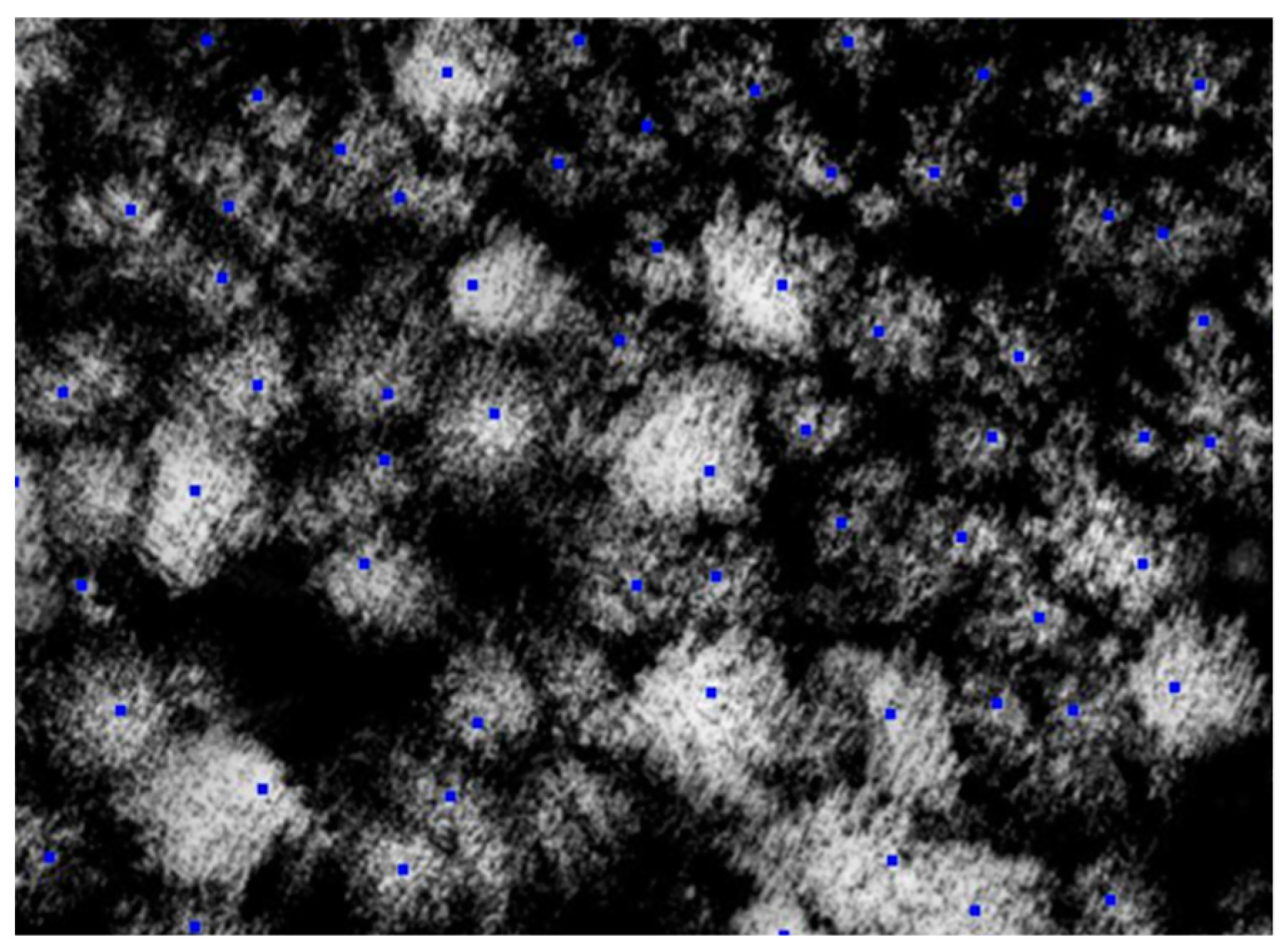
The vegetation height matrices derived from the Lidar data are used for this purpose(Figure 5). The square window of fixed size is created in the center of each matrix cell; if the maximum of the window is reached at this point, the cell coordinates are declared to be tree coordinates, i.e., the tree coordinates coincide with the coordinates of their tops. Heights are then calculated at the derived points (Figure 6), and then the coordinates of the points are deduced from the coordinates of the las-file.
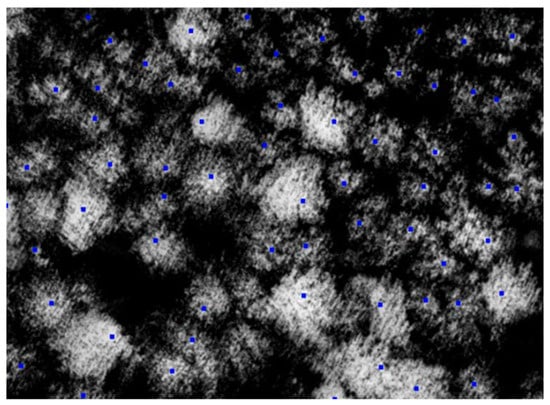
Figure 5.
Maximums found on the elevation maps (marked in blue).
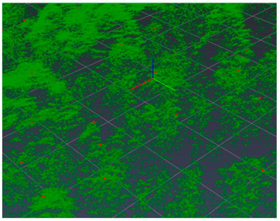
Figure 6.
Formation of the height map (dots in green are trees, in red are their maxima).
Tree Species Identification
Tree species identification was performed based on the computer vision process, consisting of expert partitioning of the tree species composition (Figure 7), training samples, and generating machine learning models based on convolutional neural networks on the YOLO architecture. Training an object-detection model such as the YOLOv5 requires a dataset containing object images and the coordinates of the bounding boxes of the objects themselves.
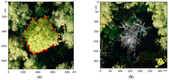
Figure 7.
Outline from expert mark-up: (a) live tree; (b) dead tree(verification of crown contours is indicated by red dots).
The species composition of the forest stand was determined from RGB images using machine learning models. The algorithm for decoding species composition using artificial intelligence (based on neural networks) was conducted as follows:
- Manual marking was completed—the operator carried out contour and analytical interpretation, as a result of which the species composition of the forest stand was determined.
- Integration of manual marking data and RGB images.
- Formation of training samples using neural network analysis.
- Testing and calibration of machine learning models created based on neural networks.
- Hyperspectral data were used to clarify the species identity and correct the breed composition.
Determination of Crown Diameter
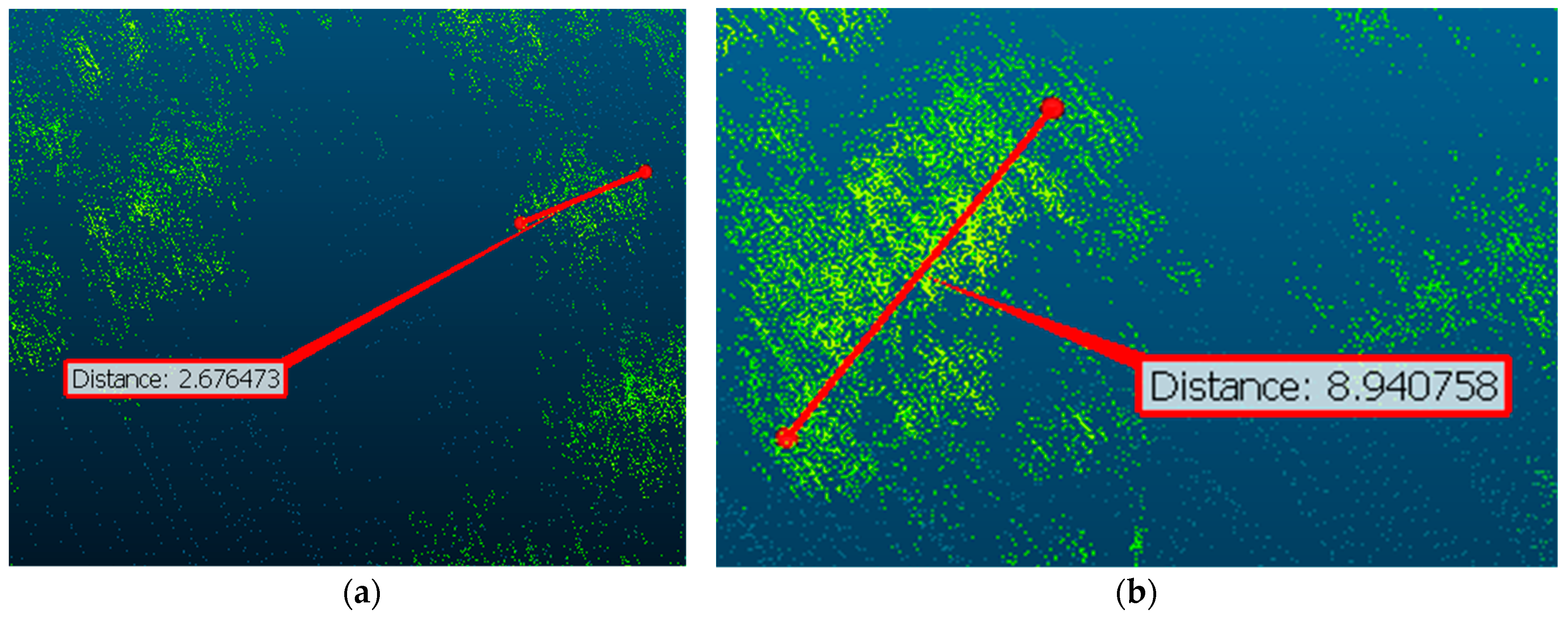
The tree crown diameter decoding process was based on the processing of point clouds obtained during the Lidar imagery processing. Knowing the coordinates (centers) of the trees, it is possible to determine both the heights and the crown diameters of individual trees. Pre-processing is performed manually in specialized point cloud software (e.g., QGIS, https://qgis.org/ru/site/ accessed on 8 May 2024) (Figure 8).
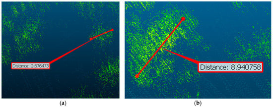
Figure 8.
Measurement of crown diameters (meters) from the Lidar data: (a) tree crown diameter on SP 13; (b) tree crown diameter on SP 3.
Following training of the AI-based on the neural network method, crown diameters were determined automatically.
Determination of Tree Height and Height of Crown Base
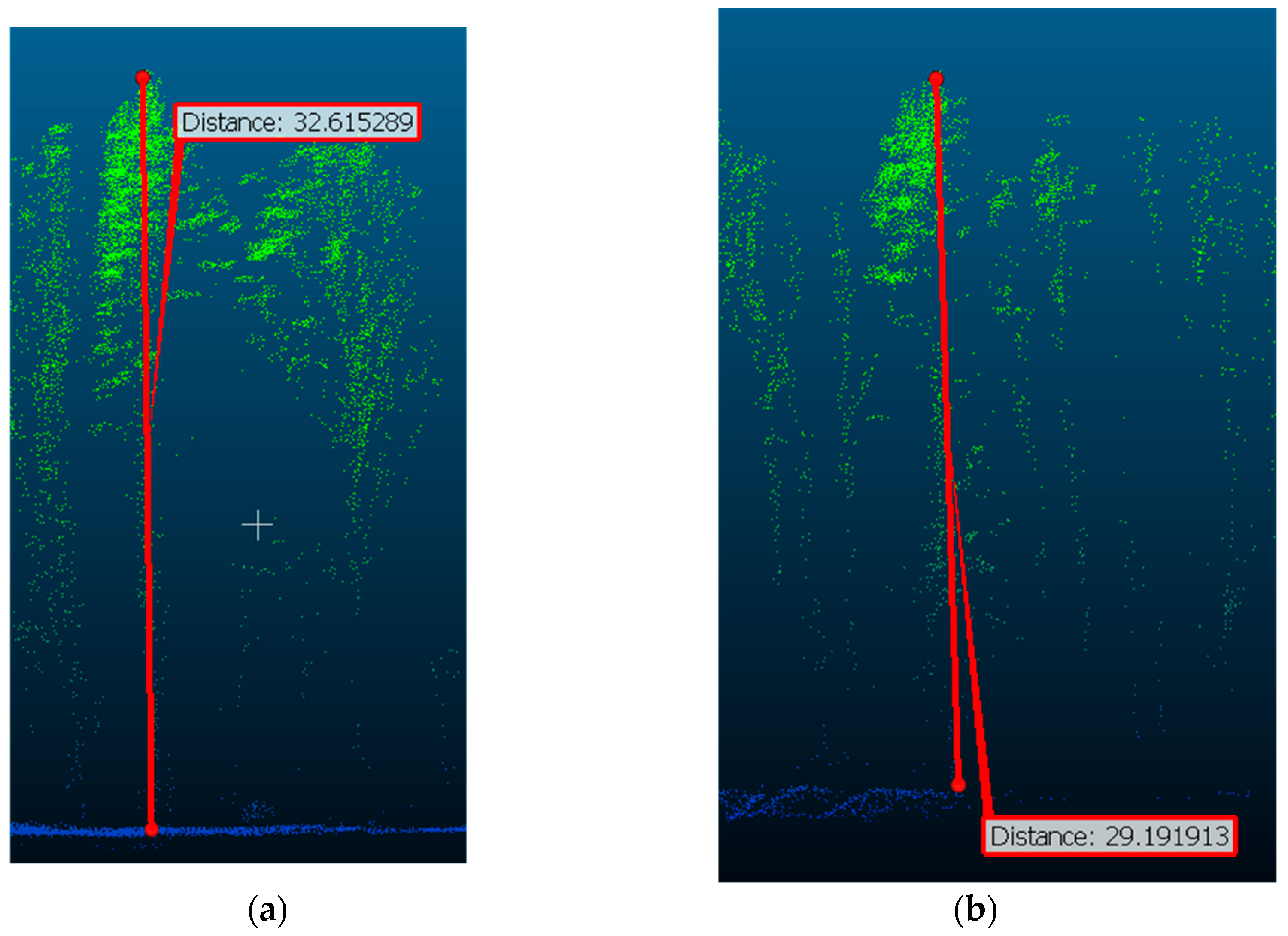
The process of determining tree heights was based on working with the Lidar point clouds. Each point cloud file contains information about the coordinates of the points, which allows us to determine the ground surface and the forest canopy; by subtracting one from the other, one candeterminethe stand height in meters (Figure 9).

Figure 9.
Measurement of tree height (meters) from the Lidar data: (a) maximum tree height on SP 8; (b) maximum tree height on SP 10.
Automated tree height estimation involves calculating ground and vegetation surfaces, and then estimation of heights is performed by subtraction of the ground surface coordinate from the vegetation surface.
3.1.3. Shrub Layer and Understory Phytomass Assessment
The shrub layer and the understory in the stand are not always fully accounted for in carbon balance estimations [65,100,101,102,103]. However, the density and height of undergrowth can have a significant impact on the carbon content of phytomass. To improve the accuracy of determining the forest stand phytomass, the scale for accounting undergrowth and undergrowth by remote sensing methods using hyperspectral and the Lidar survey data was developed.
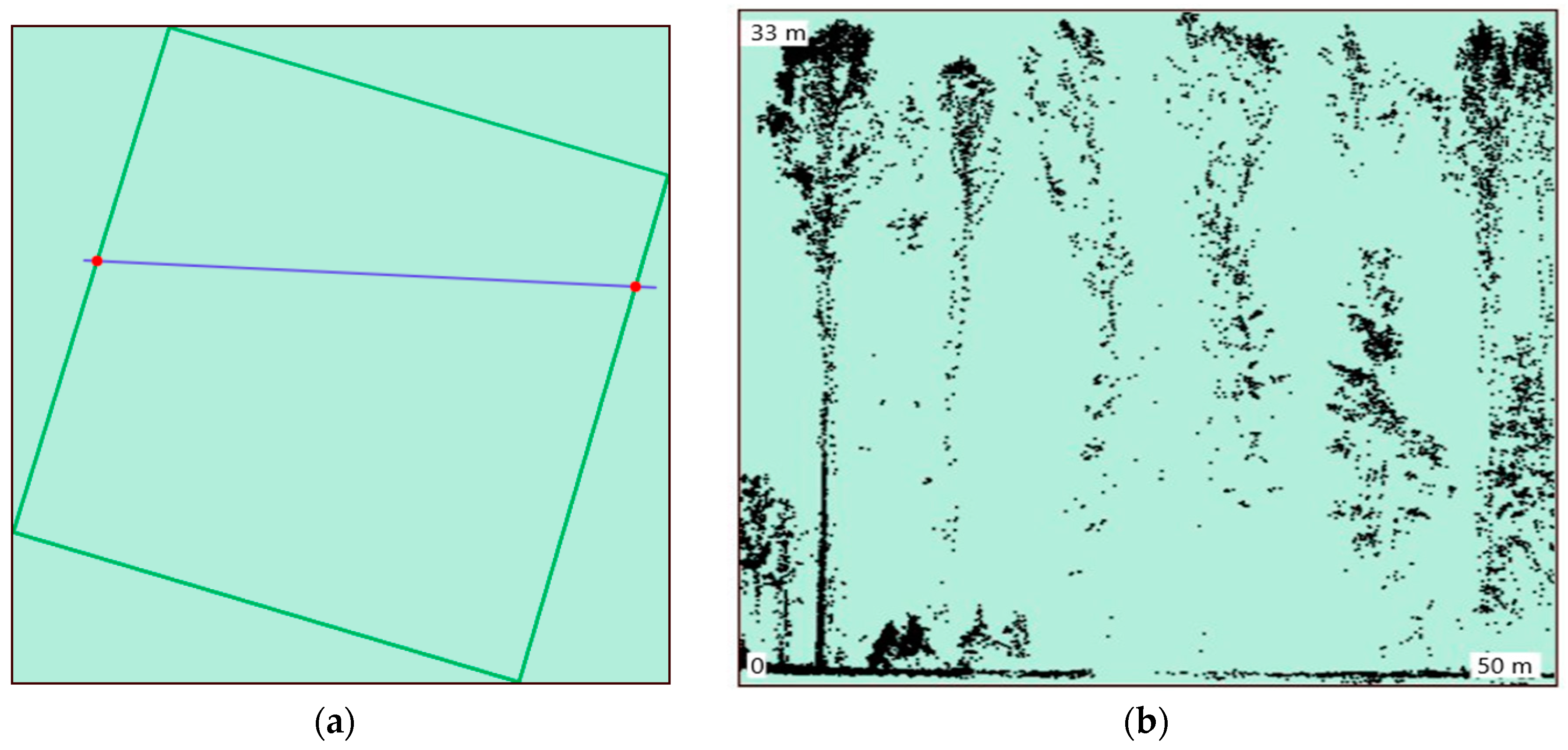
To calculate the amount of undergrowth using remote methods, a Lidar section was created (Figure 10), covering an area of 50 × 1 m. Based on the obtained value from Table 3 and Table 4, the phytomass was calculated.
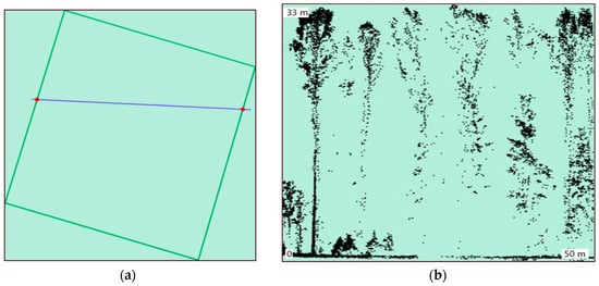
Figure 10.
Displaying of the Lidar data in the web interface: (a) general view and location of the Lidar section in the study area; (b) three-dimensional structure of the forest stand displayed as the Lidar transect.

Table 3.
Reference values of the shrub phytomass in the stands growing in the fresh forest growth conditions, kg ha−1 dry weight (range of variation/mean value).

Table 4.
Reference values of the understory phytomass in the stands growing in the fresh forest growth conditions, kg ha−1 dry weight (range of variation/mean value).
The scale was compiled on the basis of the experimental materials (field samples obtained both in this study and in earlier studies), with the application of mathematical modelling methods for interpolation and approximation of the results. The phytomass was calculated considering categories of density and height (see Table 3 and Table 4).
The Lidar transect was performed using the developed tools with the web interface shown in Figure 10a. At least three Lidar transects should be made in the studied area (Figure 10b) and then the average number of shrubs and understory should be determined.
The scientific novelty of working with hyperspectral cubes is their processing algorithm. Clustering of spectra for each image is performed; here, 2500 spectra are grouped into several clusters with the k-means clustering algorithm. The resulting median spectra are compared with the spectra of reflected light from the plants, on the basis of which they are combined into clusters. The spectra belonging to the clusters that clearly do not correspond to the plant spectra are then excluded from further consideration, while the remaining spectra are involved in computer vison methods. In partitioning mode, training samples are generated from them. The example of the complex data processing is shown below (Figure 11).
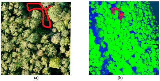
Figure 11.
Combining the RGB (a) and Lidar (b) images by common attributes.
The hyperspectral and Lidar devices provide separate categories of data to describe forests at individual tree level. The hyperspectral imagery contains meaningful plant reflectance characteristics or spectral features, while Lidar data enables the analysis of a canopy’s structural properties. Combining these two data sources improves the quality of the forest mapping (Figure 12).
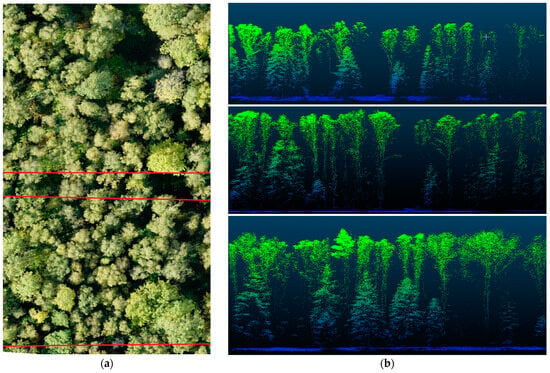
Figure 12.
Analyzed cross-section lines (a) and their mapping after processing the Lidar data (b) in stand studies.
This requires different data collection methods, appropriate processing algorithms, and classification and/or regression techniques. Remote sensing method integration aims to generate integrated information based on data with different spatial and spectral resolutions. These integrated data are more reliable and accurate than individual sources of information. Consequently, their integration improves the quality of the work and provides increased accuracy in calculating phytomass stock and estimating the carbon storage of the forest stands.
3.2. Determination of Correlations between Stand Characteristics in Order to Indirectly Identify the Deciphering Characteristics of the Forest Stand for Analytical Interpretation
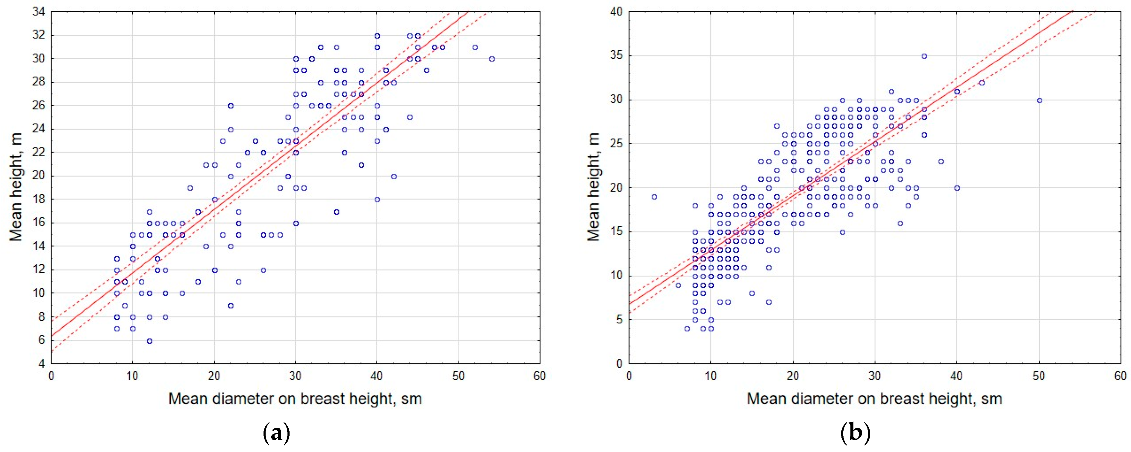
Tree stem diameter was determined by indirect methods based on the empirical data and developed regression equations. Crown diameter and tree height have a diagnostic function and are in close correlation with the stem diameter at breast height. This makes it possible to develop regression models to estimate various characteristics of individual trees, which can then be used in aerial monitoring.
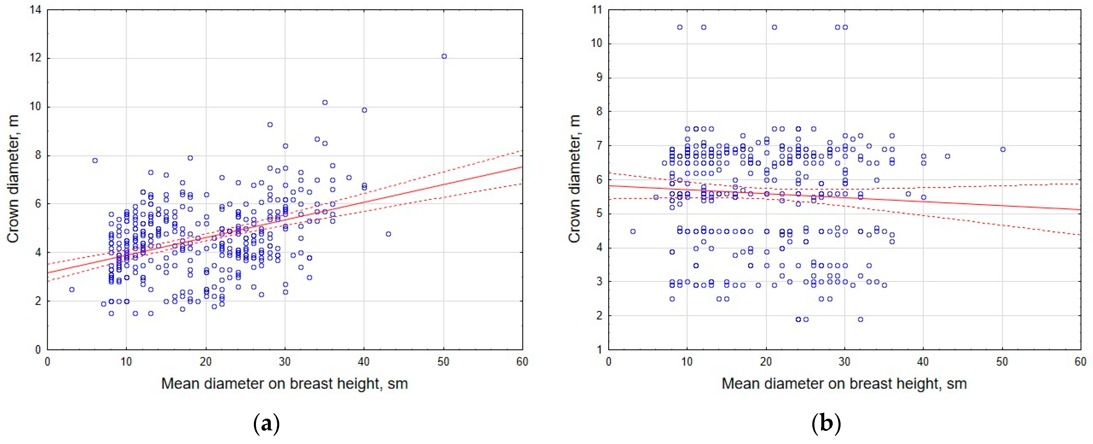
Preliminary correlation analysis of the data has shown that, for individual tree species, there is a fairly close relationship between stem diameter at 1.3 m height and crown diameter (R = 0.56 and 0.67 in coniferous and deciduous plantations, respectively) or tree height (R = 0.71 and 0.68); the strength of the relationship with the height parameter was generally higher than the corresponding relationship with crown diameter (Figure 13 and Figure 14).
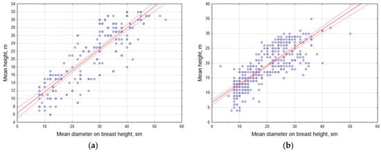
Figure 13.
Correlation of stem diameter and tree height in coniferous (a) and deciduous (b) tree stands.
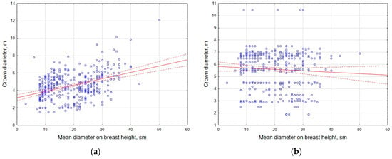
Figure 14.
Correlation of crown diameter and stem diameter in coniferous (a) and deciduous (b) tree stands.
Tree height and crown diameter are essential for remote forest monitoring since they can be accurately determined from the RGB and Lidar imagery. Based on the results of the multivariate regression analysis, models were developed to determine tree stem diameter at 1.3 m using these most informative morphometric indicators of trees (see Equation(10)). The results of the calculation of the equation coefficients are summarized in Table 5.
where Y—stem diameter at breast height 1.3 m (cm); H—tree height, m; Dcr—average crown diameter, m; a0, a1, and a2—regression coefficients.
Y = a0 + a1 H + a2 Dcr

Table 5.
Linear regression equation constants (a0–a2) for calculating stem diameter of different tree species.
The calculated coefficient of determination (R2) in the considered options exceeded 0.84 and confirmed the agreement of the linear regression models with the experimental data. The exception is oak (R2< 0.5), which requires an adjustment to the model used.
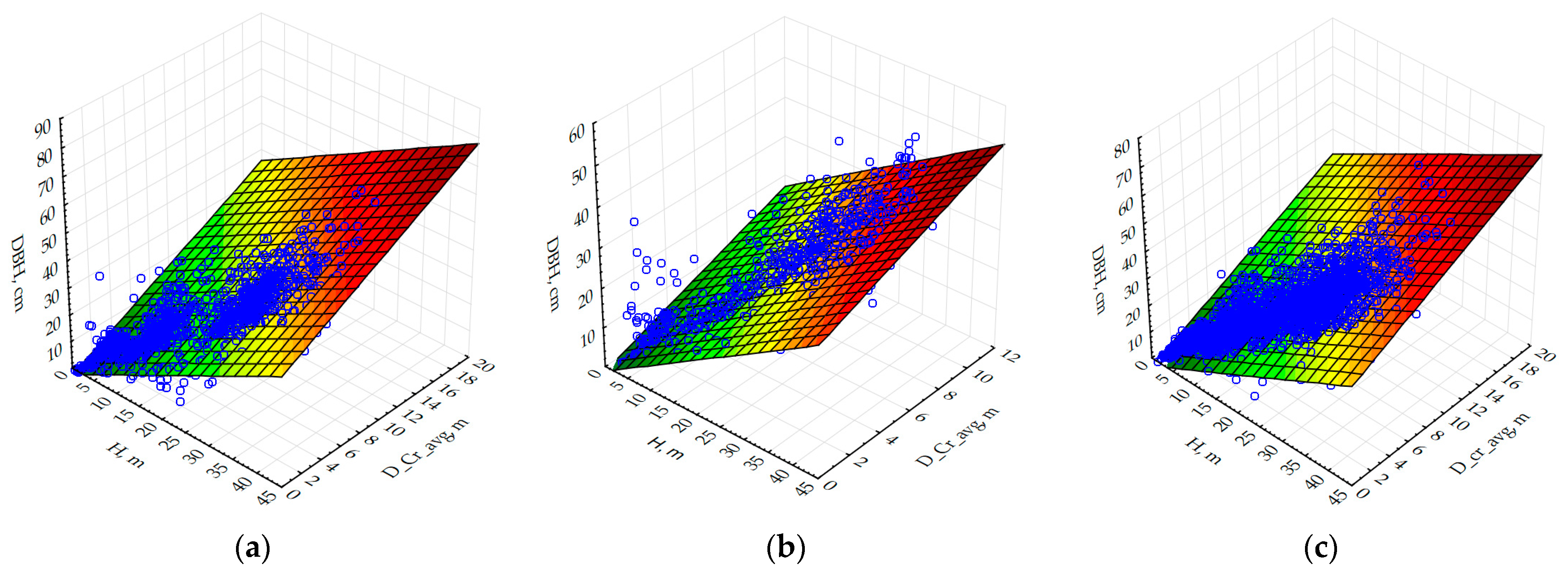
The results of the regression analysis improve the explanatory capacity of the models by 30–40% when several of the most significant morphometric indicators are used for prediction. Therefore, preference should be given to two- and multifactor models. Calculations based on the developed allometric models provide the acceptable error in determining stem diameter of almost all tree species (except for oak)—for aspen, pine, and birch, the equations provide the most accurate estimates of the considered taxation characteristics (Figure 15) and therefore could be applied in the analysis of the Lidar survey results.
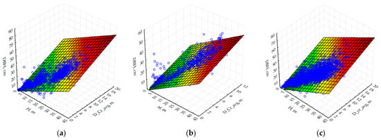
Figure 15.
Relationship between stem diameter (DBH, cm) and mean crown diameter (D_cr_avg, m) and tree height (H, m) for main tree species in the Central Forest Steppe of the East European Plain for different tree species: (a) Scots pine (Pinus sylvestris L.); (b) birch (Betula pendula L.); (c) aspen (Populus tremula L.).
3.3. Validation of the Proposed Phytomass Estimation Toolkit
The next stage of the study comprised testing the toolkit developed to determine the phytomass of the forest stands. The comparison was made between the results obtained by interpretation of imagery and the results of the ground-based inventory of trees on the sample plots.
The estimation of the phytomass by remote sensing was carried out using data on species composition and stand health (based on the RGB and hyperspectral imagery), stem diameter (derived from the allometric equations), and stand height (derived from the Lidar imagery). Average data from Table 4 and Table 5 were used to calculate understory and shrub phytomass. Additionally, dead wood was taken into account, based on the RGB and hyperspectral surveys.
The detailed data on the amount and fractional structure of phytomass obtained by ground-based inventory of sampling plots are shown in Table 6.

Table 6.
Phytomass stocks of the forest stands (age of 90–100 years) on the sample plots (SP) in the fresh forest growth conditions of the Central Forest Steppe of the East European Plain (kg ha−1 dry weight).
An analysis of Table 6 suggests that the maximum aboveground phytomass stocks in the forests of the Voronezh Region were in mixed oak–pine stands, reaching 303.0–340.3 t ha−1 (SP 1 and SP 8). Significant stocks of the aboveground phytomass (up to 309.4 t ha−1) were also found in the birch forest with ash and linden. The lowest values of the phytomass were observed predominantly in the coniferous stands (dominated by Scots pine)—up to 153.2 t ha−1 (SP 10, SP 11).
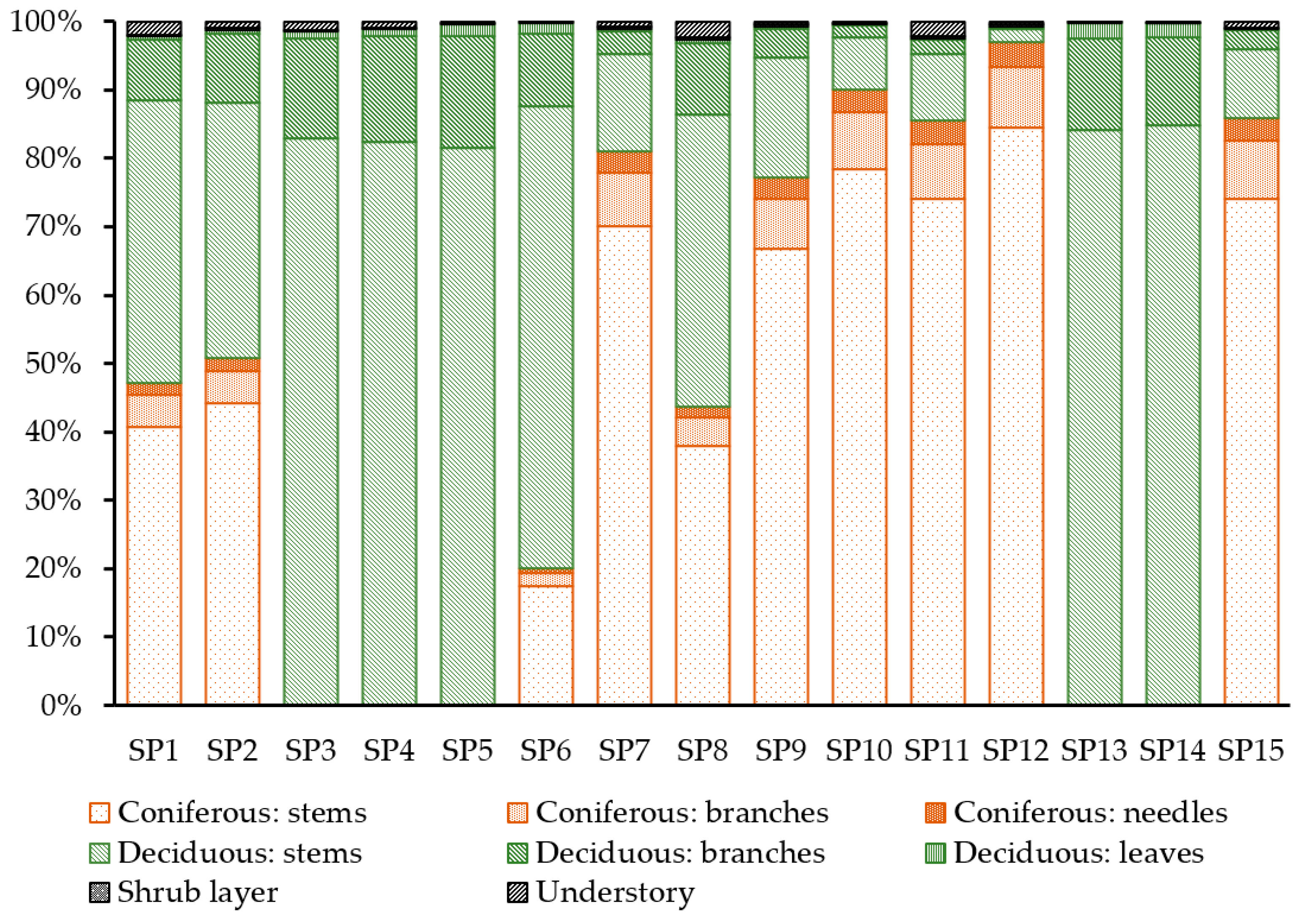
Understory and shrub layer together contribute about 1–2% of total phytomass. The lowest contribution of the lower forest layers to the total forest stand phytomass was observed in mixed birch–pine forest stands—0.2% (SP 6, SP 13)—and the highest proportion of the total phytomass was in subcanopy layers of mixed oak–pine forest stands—2.6% (SP 8) (Figure 16).
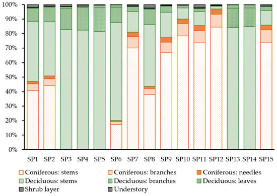
Figure 16.
Fractional composition of the phytomass on the sample plots. Sample plot numbers are marked on the horizontal axis.
Generally, the fraction in tall (over 2 m in height) undergrowth tends to be higher than in the comparable category of undergrowth. The undergrowth fraction varies over the wide range of two orders of magnitude, from 75 to 8044 kg ha−1. Contribution of the undergrowth to the total phytomass on the investigated sample plots was not significant and did not exceed 0.5%. Its stocks vary from 142 kg ha−1 in mixed birch–pine forests to 954 kg ha−1 in mixed stands with Scots pine predominance.
Stem wood accounts for at least 81% of the total phytomass of the stand. The analysis of the ratio of woody phytomass fractions clearly shows the pattern of increasing contribution of branches in mixed forests with the predominance of deciduous species, and deciduous forests—up to 15–16%—while the proportion of branches in coniferous forests accounts for less than 9–10% of total phytomass.
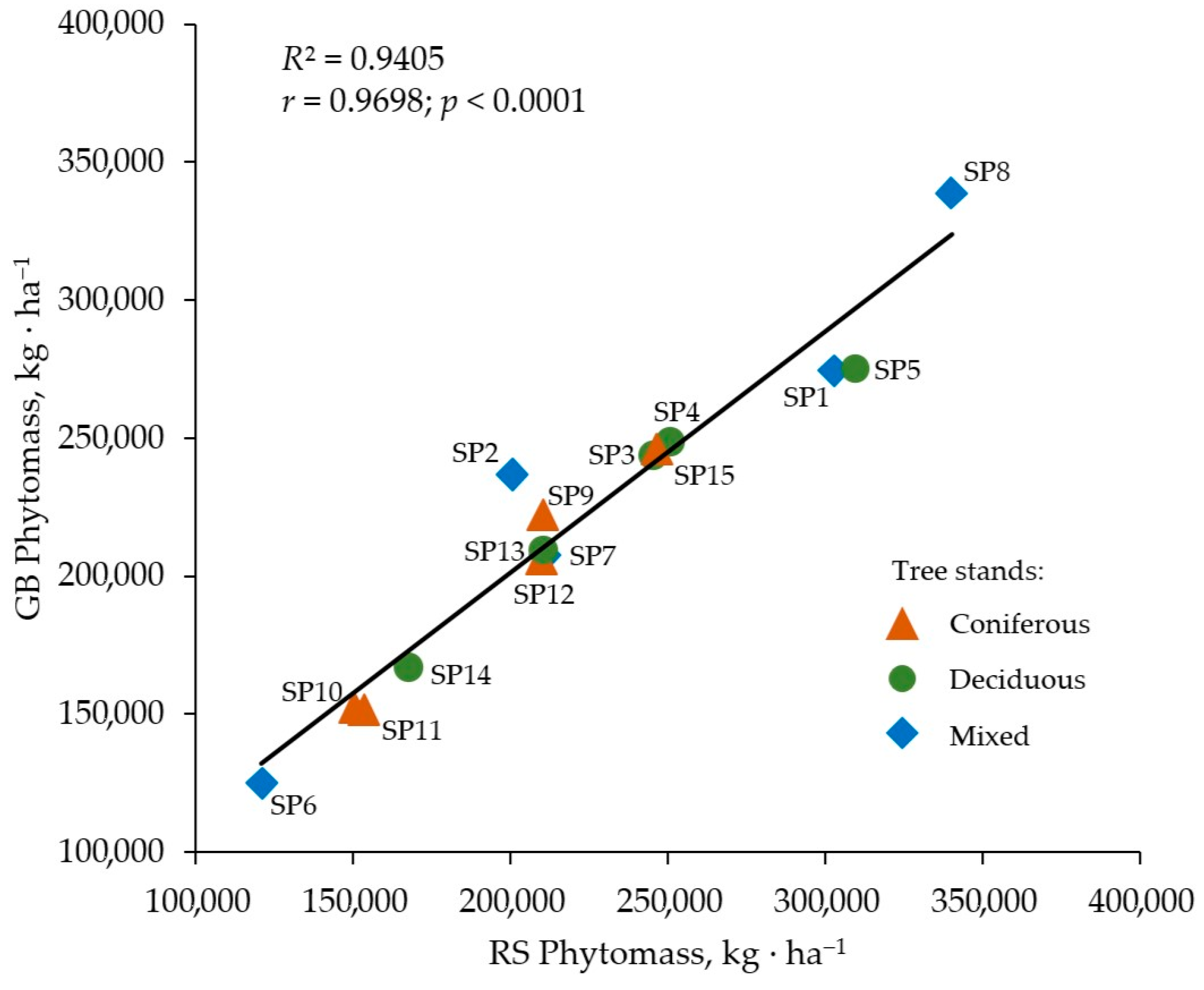
The statistical processing of the results was performed using the ANOVA (Table 7) to determine the significance of differences between the average values of the tree stand characteristics and the total amount of phytomass in stands, determined by ground-based and remote sensing methods (Figure 17).

Table 7.
Significance of differences between the mean values of phytomass in the forest stands (ta-b) determined by ground-based (a) and remote sensing (b) methods.
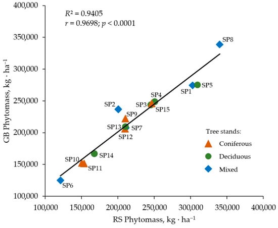
Figure 17.
Total phytomass of different tree stand types on the sample plots (SP) determined by ground-based (GB) and remote sensing (RS) methods.
Significant differences (at the significance level of p < 0.05) between the average values of the total phytomass from the ground-based and remote sensing methods were found in 33% of the cases. However, the maximum difference (observed at SP 5) in the approximation of the data did not exceed 15%. In 66% of the cases, the average phytomass values determined by the different methods did not differ significantly from each other. This demonstrates the high accuracy of the information obtained by remote sensing, using the proposed technical–methodological approach.
Remote sensing performed on the basis of the proposed methodology is comparable in accuracy to ground-based methods for determining the carbon stock in aboveground phytomass. This is achieved by taking into account undergrowthand dead wood.
The similarity of phytomass values obtained by the ground-based and the remote sensing methods was statistically confirmed: Pearson criterion χ2 (0.05; 5) = 2.79; P(χ2) = 0.68 > 0.05 was found to causeslight differences in the results of calculating phytomass by different methods. Consequently, we can reliably use the distance-based phytomass estimation technique to calculate the carbon storage of forest stands.
3.4. Calculation of Carbon Stock from Phytomass Measurements
The carbon stock calculations for the aboveground phytomass of the forest stands in the sample plots are summarized in Table 8.

Table 8.
Aboveground carbon stock of the forest stands (age of 90–100 years) on the sample plots (SP) in the fresh forest growth conditions of the Central Forest Steppe of the East European Plain (kg ha−1).
The total carbon stocks in the forest stands varied from 58.6 t ha−1 in birch-dominated stands (SP6), where minimal stem wood stocks were observed, to 167.8 t ha−1 in mixed pine-dominated stands (SP8). The shrub layer and understory contributed no more than 3.8 t C ha to the total carbon stocks. In most cases, the carbon stocks in their aboveground phytomass did not exceed 1.0 t ha−1.
4. Discussion
The hyperspectral and Lidar data complement each other. The synergy between the technologies used can be referred to as 3D-imaging spectroscopy, which has been explored in the works of several authors [104,105]. The proposed methodology is primarily based on the use of the RGB and Lidar sensors estimating as much of the forest stand phytomass as possible and allows consideration of all carbon pools for the rapid and reliable calculation of the carbon storage [106,107,108].
Similar methods for remotely estimating stands and determining the accumulation of forest phytomass using the Lidar system were used for the tree species Quercus semicarpifolia (Sm.) and Pinus roxburghii (Sarg), when calculating the carbon stock in the subtropical and temperate forests of India [108,109,110]. The proposed method was based on the assessment of ground phytomass and carbon only for the tree layer, which is not appropriate and objective when assessing forest phytocoenosis as the whole. Please note that the machine learning models used are developed on a regional basis.
In monitoring the ecological state of vegetation and carbon reserves, great importance belongs to the qualitative and quantitative characteristics of the productivity of aboveground phytomass of individual plants and phytocoenoses. Moreover, in contrast to the traditionally implemented assessment of the carbon pool in the aboveground phytomass of tree stands [33,34,64], we have studied the parameters of the accumulation of aboveground phytomass and carbon in other tiers of the forest phytocoenoses. This also indicates the feasibility and objectivity of the assessment.
In addition to the required technical and software tools, adequate methodological apparatus is required. In our case, a comprehensive technical and methodological approach was used. We believe that the assessment required data from our ground-based monitoring on the morphometric characteristics of plants and their condition. This was confirmed by a correlation analysis. Positive correlations between the morphometric parameters of the woody plants were obtained. In particular, the parameters of tree height and crown diameter are important for remote environmental monitoring of the forest phytocoenoses. They can be determined by ground-based methods and remotely (from RGB images and through Lidar surveys). Multivariate regression analysis makes it possible to develop models for determining the diameter of the tree trunk, using morphometric parameters. The values of the species-specific coefficients for the number of the tree species are given. Priority should be given to two- and multifactor models when predicting the necessary morphometric parameters of ecologically and economically valuable plants. The validation of the proposed set of tools is disclosed and explanations are given for estimating phytomass using the example of the forest phytocoenoses.
The data obtained from ground-based monitoring and remote monitoring were compared differentially for the tree stands, undergrowth, shrub layer, and in general (Table 6). The major advantage of the methodology proposed for remote monitoring and control of the carbon storage compared to existing analogues is the minimization of the amount of groundwork and, consequently, the reduction inlabor costs without loss of information quality. Reliable information on the phytomass volumes will allow for operational control of forest carbon storage, which is essential for timely management decisionmaking. The proposed methodology is useful for analyzing the possibilities of sequestration of carbon and other elements in plant phytomass and soils in forested, agricultural, and populated areas. Of great importance is the application of the described methodology for studying the ecosystem-related, ecological–protective, and phytomeliorative properties of tree stands and other vegetation elements in relation to agrophytocoenoses.
Wu et al. [111], Reinmann et al. [112], Junfang et al. [113], and thenumber of other researchers [114,115,116] believe that the quantification of the aboveground forest phytomass and carbon cycle studies in general is a highly relevant and current issue, which will provide the theoretical basis for the study of the carbon cycle and global climate change. Obtaining information on the forest ecosystems and carbon storage will make it possible to identify the inverse relationship between the processes occurring in forests and climate change. It also seems promising to analyze the state of tree plantations and forests, the accumulation of their phytomass to consider the balance of the carbon and nutrient cycles, to assess degradation processes due to environmental and climatic transformations in the environment and in the forest natural ecosystems and cultural ecosystems [117,118,119]. Data on the formation of the phytomass of the forests and plantations can be used as the basis for environmental and climate–economic management of natural and cultural ecosystems. This is consistent with the results of other authors [120,121,122,123]. This seems possible in geographically, ecologically, and economically diverse areas. The presented methodology for integrated carbon monitoring allows us to identify the ecological state, the limits of sustainability, and the resource base of the corresponding natural phytocoenoses and agrophytocoenoses. The proposed universal methodology can be of decisive importance in the selection of plant species and varieties for afforestation, landscaping, horticulture, protection, and restoration of soil ecosystems, and the protection of and increase in the resource attractiveness of landscapes on the East European Plain and other territories.
5. Conclusions
The use of UAVs for the remote sensing of forest ecosystems in the Eastern European Plain is the issue that is becoming more and more important. Estimating the amount of carbon stored in forests is the critical undertaking. At present, there is no single system that integrates the collection, storage, and analysis of data on forest ecosystem health and structure, leading to significant uncertainties in current biomass assessment methods. It is crucial to enhance existing methods and develop new approaches for estimating forest phytomass and calculating carbon stocks.
The estimation of the carbon storage of the forests is based on the calculation of the phytomass of the stand and other components of the forest ecosystem. Meanwhile, woody phytomassis based on the application of allometric equations or conversion factors, defined as the ratio of total stand phytomass (including aboveground, belowground, and understory) to the stemwood stock. The conversion factors are differentiated according to the age of the stand and other taxonomic indicators obtained by ground-based forest inventory.
In the study area, on average, up to 81% of the total volume of formed phytomass is stem wood. To complete the assessment, the contribution of other layers of forest vegetation was also established. The undergrowth and shrub layer are responsible for the formation of aboveground phytomass in the volume of up to 2% of the total volume of aboveground phytomass of forest phytocenoses. Phytocenoses of the oak, oak–pine, pine, and birch forests are natural ecological frameworks for the ecosystems they form and for the ecosystems adjacent to them. The total carbon reserves in the aboveground phytomass of phytocenoses varied, depending on their composition. The total carbon reserve reached its maximum value (163.6 t ha−1) in plantations of mixed species composition with the predominance of the pine.
To integrate and approximate data obtained during ground surveys and data obtained during remote monitoring based on the UAVs, technical and methodological tools have been developed. This toolkit allows you to analyze and decipher information. The technical and methodological tools used in forest sensing using the UAVs are based on machine learning technology using the neural network method. The proposed integrated approach makes it possible to determine taxation indicators of plantings and volumes of aboveground phytomass in the automated mode (or with elements of automation). To achieve automation of the process, data of three categories (RGB, Lidar, hyperspectrum) were collected and artificial intelligence methods based on the ultra-precise neural network were applied.
The remote determination of the main forest stands’ taxation indices and, accordingly, the volume of the phytomass of the key carbon pools will also make it possible to remotely determine the carbon storage of forest ecosystems. This will allow the remote monitoring of carbon storage over large areas.
The similarity of phytomass values obtained by ground-based and remote sensing methods was statistically confirmed: Pearson criterion χ2 (0.05; 5) = 2.79. Consequently, we can reliably use the distance-based phytomass estimation technique to calculate the carbon storage of forest stands.
The use of the UAVs with appropriate hardware will make it possible to obtain the forest characteristics necessary for the determination of the carbon storage as the need arises: to determine baseline characteristics at the start of forest climate projects, when monitoring the dynamics of carbon storage, and so on. It is also possible to determine the characteristics of forests after selective logging and after fires of different intensities. Of great importance is the possibility of using the scientific idea of the work and the described methodology to assess and predict the condition of the trees and shrubs as ecological frameworks and complex phytomeliorants on lands of different target categories. The methodological approach we propose is easily compatible with current technologies in the field of conservation, protection, and reproduction of forests in the Central Forest Steppe Region in the East European Plain. This allows the approach to be successfully integrated into the general system of forest monitoring and the assessment of stocks of wood and other plant resources, and into environmental and economic management in different types of cultural and natural ecosystems and in different landscapes.
Author Contributions
Conceptualization, V.S., M.V.L. and N.D.; methodology, V.S. and D.L.; formal analysis, V.S., S.S., S.M. and M.V.L.; investigation, V.S., S.S., S.M. and M.V.L.; data processing and analysis, A.S.; writing—original draft preparation, V.S., D.L., S.M., M.V.L., A.S. and P.L.; writing—review and editing, V.S., D.L., S.S., S.M. and M.V.L.; organizational conceptualization and administrative support, V.S. and M.V.L.; participation in correction—V.S., M.V.L. and N.D.; visualization, V.S. All authors have read and agreed to the published version of the manuscript.
Funding
This research was funded the research was carried out within the state assignment of Ministry of Science and Higher Education of the Russian Federation (theme No. FZUR-2024-0002) “Development of a technological solutions aimed at increasing the efficiency of forest fire monitoring and detailed assessment of the consequences of forest fires in the conditions of the Central forest steppe”(State contract No. 075-03-2024-166). The research was supported by the Interdisciplinary Scientific and Educational School of Moscow University “Brain, Cognitive Systems, Artificial Intelligence”.
Institutional Review Board Statement
Not applicable.
Informed Consent Statement
Not applicable.
Data Availability Statement
The data presented in this study are available on request from the corresponding author. The data are not publicly available due to privacy restrictions.
Conflicts of Interest
The authors declare no conflicts of interest.
References
- Hoegh-Guldberg, O.; Jacob, D.; Taylor, M.; Guillen Bolanos, T.; Bindi, M.; Brown, S.; Camilloni, I.; Diedhiou, A.; Djalante, R.; Ebi, K.; et al. The human imperative of stabilizing global climate change at 1.5 °C. Science 2019, 365, eaaw6974. [Google Scholar] [CrossRef] [PubMed]
- Sippel, S.; Meinshausen, N.; Fischer, E.M.; Szekely, E.; Knutti, R. Climate change now detectable from any single day of weather at global scale. Nat. Clim. Change 2020, 10, 35–41. [Google Scholar] [CrossRef]
- Malysheva, N.V.; Moiseev, B.N.; Filipchuk, A.N.; Zolina, T.A. Methods for assessing the carbon balance in forest ecosystems and the possibility of their use for calculating annual carbon sequestration. For. Bull. 2017, 21, 4–13. [Google Scholar] [CrossRef]
- Zhang, X.; Liu, D.; Ma, J.; Wang, X.; Li, Z.; Zheng, D. Visible Near-Infrared Hyperspectral Soil Organic Matter Prediction Based on Combinatorial Modeling. Agronomy 2024, 14, 789. [Google Scholar] [CrossRef]
- Braga, C.I.; Crisan, V.E.; Petritan, I.C.; Scarlatescu, V.; Vasile, D.; Lazar, G.; Petritan, A.M. Short-Term Effects of Anthropogenic Disturbances on Stand Structure, Soil Properties, and Vegetation Diversity in a Former Virgin Mixed Forest. Forests 2023, 14, 742. [Google Scholar] [CrossRef]
- Chhabra, A.; Palria, S.; Dadhwal, V.K. Spatial distribution of phytomass carbon in Indian forests. Glob. Change Biol. 2002, 8, 1230–1239. [Google Scholar] [CrossRef]
- Chen, L.; Song, M.; Song, T.-Q.; Wang, H.; Zeng, F.-P.; Peng, W.-X.; Du, H.; Han, C.; Su, L. Carbon storage and its allocation in soft broadleaved forests with different stand ages in Guangxi. Chin. J. Ecol. 2017, 36, 592–600. [Google Scholar] [CrossRef]
- Braga, C.I.; Petrea, S.; Radu, G.R.; Cucu, A.B.; Serban, T.; Zaharia, A.; Leca, S. Carbon Sequestration Dynamics in Peri-Urban Forests: Comparing Secondary Succession and Mature Stands under Varied Forest Management Practices. Land 2024, 13, 492. [Google Scholar] [CrossRef]
- Zhou, Y.; She, J.; Zhu, X. Dynamic analysis of biodiversity, carbon storage and environmental factors of coniferous forest in Loudi City, Hunan Province. Int. J. Low-Carbon Technol. 2022, 17, 831–840. [Google Scholar] [CrossRef]
- Zielonka, A.; Drewnik, M.; Musielok, Ł.; Dyderski, M.K.; Struzik, D.; Smułek, G.; Ostapowicz, K. Biotic and Abiotic Determinants of Soil Organic Matter Stock and Fine Root Biomass in Mountain Area Temperate Forests—Examples from Cambisols under European Beech, Norway Spruce, and Silver Fir (Carpathians, Central Europe). Forests 2021, 12, 823. [Google Scholar] [CrossRef]
- Bisht, S.; Bargali, S.S.; Bargali, K.; Rawat, G.S.; Rawat, Y.S.; Fartyal, A. Influence of Anthropogenic Activities on Forest Carbon Stocks—A Case Study from Gori Valley, Western Himalaya. Sustainability 2022, 14, 16918. [Google Scholar] [CrossRef]
- Diao, J.; Liu, J.; Zhu, Z.; Wei, X.; Li, M. Active forest management accelerates carbon storage in plantation forests in Lishui, southern China. For. Ecosyst. 2022, 9, 100004. [Google Scholar] [CrossRef]
- Indriyani, L.; Bana, S.; Yasin, A.; Sudia, L.B.; Kahirun; Midi, L.O. Hardin The Potential of Blue Carbon Stocks and Carbon Dioxide Absorption in Mangrove Forests to Support Low Carbon Emission Development in Southeast Sulawesi Province, Indonesia. Int. J. Adv. Sci. Eng. Inf. Technol. 2020, 10, 2526–2535. [Google Scholar] [CrossRef]
- Molotoks, A.; Stehfest, E.; Doelman, J.; Albanito, F.; Fitton, N.; Dawson, T.P.; Smith, P. Global projections of future cropland expansion to 2050 and direct impacts on biodiversity and carbon storage. Glob. Change Biol. 2018, 24, 5895–5908. [Google Scholar] [CrossRef] [PubMed]
- Payne, N.J.; Cameron, D.A.; Leblanc, J.D.; Morrison, I.K. Carbon storage and net primary productivity in Canadian boreal mixedwood stands. J. For. Res. 2019, 30, 1667–1678. [Google Scholar] [CrossRef]
- Tian, L.; Tao, Y.; Fu, W.X.; Li, T.; Ren, F.; Li, M.Y. Dynamic Simulation of Land Use/Cover Change and Assessment of Forest Ecosystem Carbon Storage under Climate Change Scenarios in Guangdong Province, China. Remote Sens. 2022, 14, 2330. [Google Scholar] [CrossRef]
- Xiao, J.F.; Chevallier, F.; Gomez, C.; Guanter, L.; Hicke, J.A.; Huete, A.R.; Ichii, K.; Ni, W.J.; Pang, Y.; Rahman, A.F.; et al. Remote sensing of the terrestrial carbon cycle: A review of advances over 50 years. Remote Sens. Environ. 2019, 233, 111383. [Google Scholar] [CrossRef]
- Strandberg, G.; Kjellström, E. Climate Impacts from Afforestation and Deforestation in Europe. Earth Interact. 2018, 23, 1–27. [Google Scholar] [CrossRef]
- Veiga, J.; Lima, A.L.; Brito, A. Effects of deforestation at different spatial scales on the climate of the Amazon basin. Clim. Res. 2023, 91, 21. [Google Scholar] [CrossRef]
- Volodkin, A.A.; Volodkina, O.A.; Larionov, M.V. Dynamics of reproduction of forest plantations in the forest-steppe zone of the Middle Volga Region. IOP Conf. Ser. Earth Environ. Sci. 2022, 979, 012101. [Google Scholar] [CrossRef]
- Chmura, D.J.; Modrzynski, J. Sensitivity of height growth response to climate change does not vary with age in common garden among Norway spruce populations from elevational gradients. For. Ecol. Manag. 2023, 542, 121118. [Google Scholar] [CrossRef]
- Sitková, Z.; Hlásny, T. Editorial to the thematic issue: Ecological interactions in Central European forest under climate change. Cent. Eur. For. J. 2020, 66, 189–190. [Google Scholar] [CrossRef]
- Vedernikov, K.E.; Bukharina, I.L.; Udalov, D.N.; Pashkova, A.S.; Larionov, M.V.; Mazina, S.E.; Galieva, A.R. The State of Dark Coniferous Forests on the East European Plain Due to Climate Change. Life 2022, 12, 1874. [Google Scholar] [CrossRef] [PubMed]
- Vinceti, B.; Manica, M.; Lauridsen, N.; Verkerk, P.J.; Lindner, M.; Fady, B. Managing forest genetic resources as a strategy to adapt forests to climate change: Perceptions of European forest owners and managers. Eur. J. For. Res. 2020, 139, 1107–1119. [Google Scholar] [CrossRef]
- Gibadulina, I.I.; Larionov, M.V.; Maslennikova, N.N. Anatomical and morphological features of the leaves of Tilia cordata Mill. as an indicator of the adaptive capabilities of the species to the conditions of the urban environment. IOP Conf. Ser. Earth Environ. Sci. 2022, 988, 032082. [Google Scholar] [CrossRef]
- Hruška, J.; Oulehle, F.; Chuman, T.; Kolář, T.; Rybníček, M.; Trnka, M.; McDowell, W.H. Forest growth responds more to air pollution than soil acidification. PLoS ONE 2023, 18, e0256976. [Google Scholar] [CrossRef]
- Larionov, M.V.; Larionov, N.V.; Siraeva, I.S.; Gromova, T.S. Ecological and aesthetic significance of an auto-trophic component of artificial ecosystems in ensuring of the environmental comfort and the public health protection. IOP Conf. Ser. Earth Environ. Sci. 2020, 421, 082002. [Google Scholar] [CrossRef]
- Larionov, M.V.; Soldatova, V.V.; Logacheva, E.A.; Larionov, N.V. An ecological analysis of the composition and condition of woody plants in urban and suburban ecosystems of the Khopyor River Region. IOP Conf. Ser. Earth Environ. Sci. 2020, 421, 062025. [Google Scholar] [CrossRef]
- Larionov, M.V.; Tarakin, A.V.; Minakova, I.V.; Sentishcheva, E.A.; Bukreeva, T.N. Creation of artificial phytocenoses with controlled properties as a tool for managing cultural ecosystems and landscapes. IOP Conf. Ser. Earth Environ. Sci. 2021, 848, 012127. [Google Scholar] [CrossRef]
- Bolte, A.; Lambertz, B.; Steinmeyer, A.; Kallweit, R.; Meesenburg, H. Zur Funktion der Bodenvegetation im Nährstoffhaushalt von Wäldern—Studien auf Dauerbeobachtungsflächen des EU Level II-Programms in Norddeutschland (The role of the herbaceous vegetation in forest nutrient cycling—Studies on permanent plots of the EU Level II program in North Germany). Forstarchiv 2004, 75, 207–220. [Google Scholar] [CrossRef]
- Davis, Z.; Nesbitt, L.; Guhn, M.; van den Bosch, M. Assessing changes in urban vegetation using Normalised Difference Vegetation Index (NDVI) for epidemiological studies. Urban For. Urban Green. 2023, 88, 128080. [Google Scholar] [CrossRef]
- Kaul, M.; Mohren, G.M.J.; Dadhwal, V.K. Phytomass carbon pool of trees and forests in India. Clim. Change 2011, 108, 243–259. [Google Scholar] [CrossRef]
- Larionov, M.V.; Volodkin, A.A.; Volodkina, O.A.; Lebedev, E.V.; Khanbabayeva, O.E.; Tazina, S.V.; Kozlova, E.A.; Orlova, E.E.; Zubik, I.N.; Bogdanova, V.D.; et al. Features of the Territorial Distribution, Composition and Structure of Phytocenoses with the Participation of Fraxinus excelsior, Their Resource Qualities, Ecological and Economic Importance (Southeastern Part of the East European Plain). Life 2023, 13, 93. [Google Scholar] [CrossRef] [PubMed]
- Lebedev, V.M.; Lebedev, E.V.; Sorokopudov, V.N.; Larionov, M.V. Root Nutrition, Photosynthesis, and Net Primary Production in Tree Stands of the genus Picea at the Organism Level within the Range in Russia. Lesn. Zhurnal 2023, 1, 38–50. [Google Scholar] [CrossRef]
- Mayer, M.; Prescott, C.E.; Abaker, W.E.A.; Augusto, L.; Cécillon, L.; Ferreira, G.W.D.; James, J.; Jandl, R.; Katzensteiner, K.; Laclau, J.-P.; et al. Tamm Review: Influence of Forest Management Activities on Soil Organic Carbon Stocks: A Knowledge Synthesis. For. Ecol. Manag. 2020, 466, 118127. [Google Scholar] [CrossRef]
- Li, D.R.; Wang, C.W.; Hu, Y.M.; Liu, S.G. General Review on Remote Sensing-Based Biomass Estimation. Geomat. Inform. Sci. Wuhan Univ. 2012, 37, 631–635. [Google Scholar] [CrossRef]
- Slavskiy, V.A.; Mironenko, A.V.; Matveev, S.M.; Litovchenko, D.A. Taxation-interpretation indicators of plantations as the basis for the development of machine learning models for remote monitoring of forests. Proc. St. Petersburg Res. Inst. For. 2022, 4, 99–114. [Google Scholar] [CrossRef]
- Ameray, A.; Bergeron, Y.; Valeria, O.; Montoro Girona, M.; Cavard, X. Forest Carbon Management: A Review of Silvicultural Practices and Management Strategies Across Boreal, Temperate and Tropical Forests. Curr. For. Rep. 2021, 7, 245–266. [Google Scholar] [CrossRef]
- Wijedasa, L.S.; Jain, A.; Ziegler, A.D.; Evans, T.A.; Fung, T. Estimating Carbon Biomass in Forests Using Incomplete Data. Biotropica 2021, 53, 397–408. [Google Scholar] [CrossRef]
- Shvidenko, A.Z.; Shepaschenko, D.G. Carbon budget of Russian forests. Sib. For. J. 2014, 1, 69–92. Available online: https://xn--80abmehbaibgnewcmzjeef0c.xn--p1ai/articles/archive/arkhiv-2014/uglerodnyy-byudzhet-lesov-rossii/ (accessed on 21 March 2024).
- Schepaschenko, D.; McCallum, I.; Shvidenko, A.; Fritz, S.; Kraxner, F.; Obersteiner, M. A new hybrid land cover dataset for Russia: A methodology for integrating statistics, remote sensing and in-situ information. J. Land Use Sci. 2011, 6, 245–259. [Google Scholar] [CrossRef]
- Pilli, R.; Alkama, R.; Cescatti, A.; Kurz, W.A.; Grassi, G. The European Forest Carbon Budget under Future Climate Conditions and Current Management Practices. Biogeosciences 2022, 19, 3263–3284. [Google Scholar] [CrossRef]
- Liang, L.; Geng, D.; Yan, J.; Qiu, S.; Shi, Y.; Wang, S.; Wang, L.; Zhang, L.; Kang, J. Remote Sensing Estimation and Spatiotemporal Pattern Analysis of Terrestrial Net Ecosystem Productivity in China. Remote Sens. 2022, 14, 1902. [Google Scholar] [CrossRef]
- Heath, L.; Nichols, M.; Smith, J.; Mills, J. FORCARB2. An Updated Version of U.S. Forest Carbon Budget Model; General Technical Report; NRS-67 USDA Forest Service, Northern Research Station: Newtown Square, PA, USA, 2010; 52p, Available online: http://nrs.fs.fed.us/pubs/35613 (accessed on 21 March 2024).
- Liu, S.; Bond-Lamberty, B.; Hicke, J.A. Simulation the impacts of disturbances on forest carbon cycling in North America: Processes, data, models and challenges. J. Geophys. Res. 2011, 116, 22. [Google Scholar] [CrossRef]
- Ma, L.; Hurtt, G.; Tang, H.; Lamb, R.; Lister, A.; Chini, L.; Dubayah, R.; Armston, J.; Campbell, E.; Duncanson, L.; et al. Spatial heterogeneity of global forest aboveground carbon stocks and fluxes constrained by spaceborne lidar data and mechanistic modeling. Glob. Change Biol. 2023, 29, 3378–3394. [Google Scholar] [CrossRef] [PubMed]
- Vahedi, A.A. Monitoring soil carbon pool in the Hyrcanian coastal plain forest of Iran: Artificial neural network application in comparison with developing traditional models. CATENA 2017, 152, 182–189. [Google Scholar] [CrossRef]
- Yu, Y.; Guo, B.; Wang, C.; Zang, W.; Huang, X.; Wu, Z.; Xu, M.; Zhou, K.; Li, J.; Yang, Y. Carbon storage simulation and analysis in Beijing-Tianjin-Hebei region based on CA-plus model under dual-carbon background. Geomat. Nat. Hazards Risk 2023, 14, 1. [Google Scholar] [CrossRef]
- Nyamukuru, A.; Whitney, C.; Tabuti, J.R.S.; Esaete, J.; Low, M. Allometric models for aboveground biomass estimation of small trees and shrubs in African savanna ecosystems. Trees For. People 2023, 11, 100377. [Google Scholar] [CrossRef]
- Sarker, M.L.R.; Nichol, J.; Iz, H.B.; Bin Ahmad, B.; Rahman, A.A. Forest Biomass Estimation Using Texture Measurements of High-Resolution Dual-Polarization C-Band SAR Data. IEEE Trans. Geosci. Remote 2013, 51, 3371–3384. [Google Scholar] [CrossRef]
- Ali, A.; Lin, S.L.; He, J.K.; Kong, F.M.; Yu, J.H.; Jiang, H.S. Climate and soils determine aboveground biomass indirectly via species diversity and stand structural complexity in tropical forests. For. Ecol. Manag. 2019, 432, 823–831. [Google Scholar] [CrossRef]
- Strategy for the Development of the Forest Complex of the Russian Federation until 2023 (Decree of the Government of the Russian Federation dated 11 February 2021 No. 312-r). Available online: https://docs.cntd.ru/document/573658653 (accessed on 1 September 2023).
- Deng, L.; Liu, S.G.; Kim, D.G.; Peng, C.H.; Sweeney, S.; Shangguan, Z.P. Past and future carbon sequestration benefits of China’s grain for green program. Glob. Environ. Change 2017, 47, 13–20. [Google Scholar] [CrossRef]
- Gong, W.; Sun, J.; Shi, S.; Yang, J.; Du, L.; Zhu, B.; Song, S. Investigating the Potential of Using the Spatial and Spectral Information of Multispectral LiDAR for Object Classification. Sensors 2015, 15, 21989–22002. [Google Scholar] [CrossRef] [PubMed]
- Slavskiy, V.A.; Matveev, S.M. Some aspects of the laying of permanent trial plots during the state inventory of forests. Lesotechnical J. 2021, 11, 56–63. [Google Scholar] [CrossRef] [PubMed]
- Huang, H.B.; Liu, C.X.; Wang, X.Y.; Zhou, X.L.; Gong, P. Integration of multi-resource remotely sensed data and allometric models for forest aboveground biomass estimation in China. Remote Sens. Environ. 2019, 221, 225–234. [Google Scholar] [CrossRef]
- Zhang, R.; Zhou, X.H.; Ouyang, Z.T.; Avitabile, V.; Qi, J.G.; Chen, J.Q.; Giannico, V. Estimating aboveground biomass in subtropical forests of China by integrating multisource remote sensing and ground data. Remote Sens. Environ. 2019, 232, 111341. [Google Scholar] [CrossRef]
- Zhang, Y.Z.; Liang, S.L.; Yang, L. A Review of Regional and Global Gridded Forest Biomass Datasets. Remote Sens. 2019, 11, 2744. [Google Scholar] [CrossRef]
- Chopping, M.; Wang, Z.S.; Schaaf, C.; Bull, M.A.; Duchesne, R.R. Forest aboveground biomass in the southwestern United States from a MISR multi-angle index, 2000–2015. Remote Sens. Environ. 2022, 275, 112964. [Google Scholar] [CrossRef]
- Li, Y.; Xiao, J.; Cong, N.; Yu, X.; Lin, Y.; Liu, T.; Qi, G.; Ren, P. Modeling Ecological Resilience of Alpine Forest under Climate Change in Western Sichuan. Forests 2023, 14, 1769. [Google Scholar] [CrossRef]
- Zhang, Z.; Tian, X.; Chen, R.X.; He, Q.S. Review of methods on estimating forest above ground biomass. J. Beijing For. Univ. 2011, 33, 144–150. Available online: https://www.researchgate.net/publication/286837566_Review_of_methods_on_estimating_forest_above_ground_biomass (accessed on 21 March 2024).
- Demina, N.A.; Karpov, A.A.; Voronin, V.V.; Lopatin, E.V.; Bogdanov, A.P. Possible use of remote sensing for reforestation processes in Arctic zone of European Russia. Arct. Environ. Res. 2018, 18, 106–113. [Google Scholar] [CrossRef]
- Malysheva, N.V.; Zolina, T.A.; Dedova, V.Y. Estimation of carbon accumulation by Russian forests: Geospatial aspect. InterCarto InterGIS 2017, 1, 373–382. [Google Scholar] [CrossRef][Green Version]
- Filipchuk, A.N.; Moiseev, B.N.; Malysheva, N.V. Methodology for taking into account the absorption of CO2 by forests in Russia. In Proceedings of the 2nd International Scientific and Technical Conference “Forests of Russia: Politics, Industry, Science, Education”, St. Petersburg, Russia, 24–26 May 2017; Volume 2, pp. 155–158. [Google Scholar]
- Baccini, A.; Walker, W.; Carvalho, L.; Farina, M.; Sulla-Menashe, D.; Houghton, R.A. Tropical forests are a net carbon source based on aboveground measurements of gain and loss. Science 2017, 358, 230–233. [Google Scholar] [CrossRef] [PubMed]
- Beaudoin, A.; Bernier, P.Y.; Guindon, L.; Villemaire, P.; Guo, X.J.; Stinson, G.; Bergeron, T.; Magnussen, S.; Hall, R.J. Mapping attributes of Canada’s forests at moderate resolution through kNN and MODIS imagery. Can. J. For. Res. 2014, 44, 521–532. [Google Scholar] [CrossRef]
- Dube, T.; Mutanga, O. Evaluating the utility of the medium-spatial resolution Landsat 8 multispectral sensor in quantifying aboveground biomass in uMgeni catchment, South Africa. ISPRS J. Photogramm. 2015, 101, 36–46. [Google Scholar] [CrossRef]
- Powell, S.L.; Cohen, W.B.; Healey, S.P.; Kennedy, R.E.; Moisen, G.G.; Pierce, K.B.; Ohmann, J.L. Quantification of live aboveground forest biomass dynamics with Landsat time-series and field inventory data: A comparison of empirical modeling approaches. Remote Sens. Environ. 2010, 114, 1053–1068. [Google Scholar] [CrossRef]
- Fremout, T.; Vinatea, J.C.D.; Thomas, E.; Huaman-Zambrano, W.; Salazar-Villegas, M.; de la Fuente, D.L.; Bernardino, P.N.; Atkinson, R.; Csaplovics, E.; Muys, B. Site-specific scaling of remote sensing-based estimates of woody cover and aboveground biomass for mapping long-term tropical dry forest degradation status. Remote Sens. Environ. 2022, 276, 113040. [Google Scholar] [CrossRef]
- Fan, W.Y.; Li, M.Z.; Yang, J.M. Forest Biomass Estimation Models of Remote Sensing in Changbai Mountain Forests. Sci. Silvae Sinicae 2011, 47, 16–20. [Google Scholar] [CrossRef]
- Hopkinson, C.; Chasmer, L.; Gynan, C.; Mahoney, C.; Sitar, M. Multisensor and Multispectral LiDAR Characterization and Classification of a Forest Environment. Can. J. Remote Sens. 2016, 42, 501–520. [Google Scholar] [CrossRef]
- Zou, X.; Zhao, G.; Li, J.; Yang, Y.; Fang, Y. 3D Land Cover Classification Based on Multispectral Lidar Point Clouds. Int. Arch. Photogramm. Remote Sens. Spatial Inf. Sci. 2016, XLI-B1, 741–747. [Google Scholar] [CrossRef]
- Kukkonen, M.; Maltamo, M.; Korhonen, L.; Packalen, P. Multispectral Airborne LiDAR Data in the Prediction of Boreal Tree Species Composition. IEEE Trans. Geosci. Remote Sens. 2019, 57, 3462–3471. [Google Scholar] [CrossRef]
- Dalponte, M.; Ene, L.T.; Gobakken, T.; Næsset, E.; Gianelle, D. Prediction of Forest Attributes with Multispectral Lidar Data. In Proceedings of the IGARSS 2018—2018 IEEE International Geoscience and Remote Sensing. Symposium, Valencia, Spain, 22–27 July 2018; pp. 7528–7531. [Google Scholar] [CrossRef]
- Dalla Corte, A.P.; Souza, D.V.; Rex, F.E.; Sanquetta, C.R.; Mohan, M.; Silva, C.A.; Almeyda-Zambrano, A.M.; Prata, G.; de Almeida, D.R.; Trautenmüller, J.W.; et al. Forest inventory with high-density UAV-Lidar: Machine learning approaches for predicting individual tree attributes. Comput. Electron. Agric. 2020, 179, 105815. [Google Scholar] [CrossRef]
- Immitzera, M.; Stepperb, C.; Böcka, S.; Straubb, C.; Atzbergera, C. Use of WorldView-2 stereo imagery and National Forest Inventory data for wall-to-wall mapping of growing stock. For. Ecol. Manag. 2016, 359, 232–246. [Google Scholar] [CrossRef]
- Shang, C.; Coops, N.C.; Wulder, M.A.; White, J.C.; Hermosilla, T. Update and spatial extension of strategic forest inventories using time series remote sensing and modeling. Int. J. Appl. Earth Obs. Geoinf. 2020, 84, 1229–1241. [Google Scholar] [CrossRef]
- Liang, X.; Hyyppä, J.; Kaartinen, H.; Lehtomäki, M.; Pyörälä, J.; Pfeifer, N.; Holopainen, M.; Brolly, G.; Pirotti, F.; Hackenberg, J.; et al. International benchmarking of terrestrial laser scanning approaches for forest inventories. ISPRS J. Photogramm. Remote Sens. 2018, 144, 137–179. [Google Scholar] [CrossRef]
- Noordermeer, L.; Gobakken, T.; Næsset, E.; Bollandsas, O.-M. Predicting and mapping site index in operational forest inventories using bitemporal airborne laser scanner data. For. Ecol. Manag. 2020, 457, 117768. [Google Scholar] [CrossRef]
- Lu, D.S.; Chen, Q.; Wang, G.X.; Liu, L.J.; Li, G.Y.; Moran, E. A survey of remote sensing-based aboveground biomass estimation methods in forest ecosystems. Int. J. Digit. Earth. 2016, 9, 63–105. [Google Scholar] [CrossRef]
- Morsy, S.; Shaker, A.; El-Rabbany, A.; LaRocque, P.E. Airborne multispectral lidar data for land-cover classification and land/water mapping using different spectral indexes. ISPRS Ann. Photogramm. Remote Sens. Spat. Inf. Sci. 2016, 3, 217–224. [Google Scholar] [CrossRef]
- Budei, B.C.; St-Onge, B.; Hopkinson, C.; Audet, F.A. Identifying the genus or species of individual trees using a three-wavelength airborne lidar system. Remote Sens. Environ. 2018, 204, 632–647. [Google Scholar] [CrossRef]
- Ekhtari, N.; Glennie, C.; Fernandez-Diaz, J.C. Classification of Airborne Multispectral Lidar Point Clouds for Land Cover Mapping. IEEE J. Sel. Top. Appl. Earth Obs. Remote Sens. 2018, 11, 2068–2078. [Google Scholar] [CrossRef]
- Wichmann, V.; Bremer, M.; Lindenberger, J.; Rutzinger, M.; Georges, C.; Petrini-Monteferri, F. Evaluating the potential of multispectral airborne lidar for topographic mapping and land cover classification. ISPRS Ann. Photogram. Remote Sens. Spat. Inform. Sci. 2015, 3, 113–119. [Google Scholar] [CrossRef]
- Shokurov, A.V. System for remote size-adaptive variable detail raster image fragment retriever. Probl. Inform. 2012, 1, 25–39. Available online: https://cyberleninka.ru/article/n/sistema-udalennogo-izvlecheniya-fragmenta-rastrovogo-izobrazheniya-izmenyaemoy-detalizatsii-adaptirovannaya-k-ego-razmeru (accessed on 21 March 2024).
- Shokurov, A.V. Irregularly Detailed Raster Image Coding Software Design with Respect to Adaptive and Interactive Image Analysis. Softw. Eng. 2011, 5, 17–28. Available online: http://iipo.tu-bryansk.ru/fileadmin/user_upload/_content_admins/Journal_PrI/ZHurnal_Programmnaja_Inzhenerija_2011_No_5.pdf (accessed on 21 March 2024).
- Rules of Sanitary Safety in Forests: Decree of the Government of the Russian Federation of 9 December 2020 No. 2047. On the Rules of Sanitary Safety in Forests//Collection of Legislation. 2020. Available online: http://docs.cntd.ru/document/436736467 (accessed on 1 September 2023).
- Lukina, N.V.; Tikhonova, E.V.; Danilova, M.A.; Bakhmet, O.N.; Kryshen, A.M.; Tebenkova, D.N.; Kuznetsova, A.I.; Smirnov, V.E.; Braslavskaya, T.Y.; Gornov, A.V.; et al. Associations between forest vegetation and the fertility of soil organic horizons in northwestern Russia. For. Ecosyst. 2019, 6, 34. [Google Scholar] [CrossRef]
- Order of the Federal Forestry Agency. On Approval of Guidelines for the State Forest Inventory. 10 November 2011. Available online: http://docs.cntd.ru/document/436736785 (accessed on 3 September 2023).
- Slavskiy, V.; Litovchenko, D.; Matveev, S.; Sheshnitsan, S.; Larionov, M.V. Assessment of Biological and Environmental Factors Influence on Fire Hazard in Pine Forests: A Case Study in Central Forest-Steppe of the East European Plain. Land 2023, 12, 103. [Google Scholar] [CrossRef]
- Order of the Ministry of Natural Resources and Ecology of the Russian Federation dated December 29, 2021 No. 1024 “On Approval of the Rules for Reforestation, the Form, Composition, Procedure for Approving a Reforestation Project, Grounds for Refusing to Approve it, as well as Requirements for the Format in the Electronic Form of a Reforestation Project”. Available online: https://docs.cntd.ru/document/728111110 (accessed on 4 September 2023).
- On Approval of the Forest Management Instruction/Order of the Ministry of Natural Resources of Russia (Ministry of Natural Resources and Ecology of the Russian Federation) dated August 05 2022 No. 510. Available online: http://publication.pravo.gov.ru/Document/View/0001202209300058 (accessed on 4 September 2023).
- Usoltsev, V.A.; Shobairi, S.O.R.; Chasovskikh, V.P. Comparing of Allometric Models of Single-tree Biomass Intended for Airborne Laser Sensing and Terrestrial Taxation of Carbon Pool in the Forests of Eurasia. Nat. Resour. Model. 2019, 32, e12187. [Google Scholar] [CrossRef]
- Utkin, A.I.; Zamolodchikov, D.G.; Gulbe, T.A.; Gulbe, Y.A. Allometric equations for phytomass based on the data on pine, spruce, birch and aspen trees in European Russia. Lesovedenie 1996, 6, 36–46. Available online: https://elibrary.ru/item.asp?id=21266850 (accessed on 21 March 2024).
- STATISTICA (13.0-StatSoft, 2021). Available online: https://statsoftstatistica.ru/ (accessed on 4 September 2023).
- Tian, X.; Yan, M.; van der Tol, C.; Li, Z.; Su, Z.B.; Chen, E.X.; Li, X.; Li, L.H.; Wang, X.F.; Pan, X.D.; et al. Modeling forest above-ground biomass dynamics using multi-source data and incorporated models: A case study over the qilian mountains. Agric. For. Meteorol. 2017, 246, 1–14. [Google Scholar] [CrossRef]
- Mehtatalo, L.; Lappi, J. Biometry for Forestry and Environmental Data: With Examples in R, 1st ed.; Chapman and Hall/CRC: New York, NY, USA, 2020. [Google Scholar] [CrossRef]
- Lüdecke, D.; Makowski, D.; Waggoner, P.; Patil, I. Assessment of Regression Models Performance; CRAN: Indianapolis, IN, USA, 2020. [Google Scholar] [CrossRef]
- Wang, J.; Yan, M.; Huang, Q.; Huang, R.; Zheng, Q. Diameter Distribution of Semi-natural Mixed Forest of Pinus massoniana and Broadleaved Trees Based on Stratification. For. Res. 2021, 34, 72–80. [Google Scholar] [CrossRef]
- Yu, C.; Mao, J.-H.; Huang, X.; Zhang, Y. Carbon capture by phytomass storage and trading to mitigate climate change and preserve natural resources. Environ. Sustain. Indic. 2024, 22, 100358. [Google Scholar] [CrossRef]
- GOST R 59328-2021 Topographic Aerial Photography. “Technical Requirements”. Standartinform. 2021. Available online: https://rkc56.ru/attach/orenburg/docs/kodeks/gost_r_59328-2021-aerofotosemka.pdf (accessed on 4 September 2023).
- Yang, B.; Zhang, W.; Lu, Y.; Zhang, W.; Wang, Y. Carbon Storage Dynamics of Secondary Forest Succession in the Central Loess Plateau of China. Forests 2019, 10, 342. [Google Scholar] [CrossRef]
- Fatehi, P.; Damm, A.; Schaepman, M.E.; Kneubuhler, M. Estimation of Alpine Forest Structural Variables from Imaging Spectrometer Data. Remote Sens. 2015, 7, 16315–16338. [Google Scholar] [CrossRef]
- Zhang, G.; Ganguly, S.; Nemani, R.R.; White, M.A.; Milesi, C.; Hashimoto, H.; Wang, W.L.; Saatchi, S.; Yu, Y.F.; Myneni, R.B. Estimation of forest aboveground biomass in California using canopy height and leaf area index estimated from satellite data. Remote Sens. Environ. 2014, 151, 44–56. Available online: https://scholar.google.com/scholar_lookup?title=Estimation+of+forest+aboveground+biomass+in+California+using+canopy+height+and+leaf+area+index+estimated+from+satellite+data&author=Zhang,+G.&author=Ganguly,+S.&author=Nemani,+R.R.&author=White,+M.A.&author=Milesi,+C.&author=Hashimoto,+H.&author=Wang,+W.L.&author=Saatchi,+S.&author=Yu,+Y.F.&author=Myneni,+R.B.&publication_year=2014&journal=Remote+Sens.+Environ.&volume=151&pages=44%E2%80%9356&doi=10.1016/j.rse.2014.01.025 (accessed on 10 February 2024). [CrossRef]
- Levick, S.R.; Shendryk, Y.; Setterfield, S.A.; Rossiter-Rachor, N.A. Evaluation of Satellite Remote Sensing Pathways for Mapping and Monitoring of Gamba Grass for the Savanna Fire Management Methodology; CSIRO and Charles Darwin University: Darwin, Australia, 2018; Volume 20, 27p, Available online: https://nesplandscapes.edu.au/wp-content/uploads/2019/10/Evaulation-of-remote-sensing-for-mapping-monitoring-gamba.pdf (accessed on 10 February 2024).
- Hill, S.; Latifi, H.; Heurich, M.; Müller, J. Individual-tree- and stand-based development following natural disturbance in a heterogeneously structured forest: A LiDAR-based approach. Ecol. Inform. 2017, 38, 12–25. [Google Scholar] [CrossRef]
- Marselis, S. Mapping Forest Fuel Structure with LiDAR; Australian National University Press: Canberra, Australia, 2014; pp. 1–35. [Google Scholar]
- Pierfranco Costabile, P.; Carmelina Costanzo, C.; Gianluca De Lorenzo, G.; De Santis, R.; Penna, N.; Macchione, F. Terrestrial and airborne laser scanning and 2-D modelling for 3-D flood hazard maps in urban areas: New opportunities and perspectives. Environ. Model. Softw. 2021, 135, 104889. [Google Scholar] [CrossRef]
- Patil, P.; Dutta, D.; Biradar, C.; Singh, M. Quantification of the terrestrial phytomass and carbon in the mountainous forest ecosystem using remote sensing and in-situ observations. Int. Arch. Photogramm. Remote Sens. Spatial Inf. Sci. 2015, XL-7/W3, 483–487. [Google Scholar] [CrossRef]
- Heyojoo, B.P.; Nandy, S. Estimation of above-ground phytomass and carbon in tree resources outside the forest (TROF): A geo-spatial approach. Banko Janakari 2015, 24, 34–40. [Google Scholar] [CrossRef][Green Version]
- Tian, L.; Wu, X.; Tao, Y.; Li, M.; Qian, C.; Liao, L.; Fu, W. Review of Remote Sensing-Based Methods for Forest Aboveground Biomass Estimation: Progress, Challenges, and Prospects. Forests 2023, 14, 1086. [Google Scholar] [CrossRef]
- Reinmann, A.B.; Smith, I.A.; Thompson, J.R.; Hutyra, L.R. Urbanization and fragmentation mediate temperate forest carbon cycle response to climate. Environ. Res. Lett. 2020, 15, 114036. [Google Scholar] [CrossRef]
- Zhao, J.; Liu, D.; Zhu, Y.; Peng, H.; Xie, H. A review of forest carbon cycle models on spatiotemporal scales. J. Clean. Prod. 2022, 339, 130692. [Google Scholar] [CrossRef]
- Liu, D.; Yan, H.; Yu, C.L.; Yin, S.P.; Wang, C.W.; Gong, L.J. Quantitative Assessment of Climate Change Impacts on Forest Ecosystems Get access Arrow. For. Sci. 2022, 69, 143–157. [Google Scholar] [CrossRef]
- Singh, K.; Sharma, P.C. Above-ground tree outside forest (TOF) phytomass and carbon estimation in the semi-arid region of southern Haryana: A synthesis approach of remote sensing and field data. J. Earth Syst. Sci. 2013, 121, 1469–1482. [Google Scholar] [CrossRef]
- Suthari, S.; Raju, V.S.; Singh, S. An assessment of the aboveground phytomass and carbon levels of the forests of northern Telangana, India, using a geospatial technique. Biodiversity 2020, 21, 227–237. [Google Scholar] [CrossRef]
- Mudrák, O.; Angst, Š.; Angst, G.; Veselá, H.; Schnablová, R.; Herben, T.; Frouz, J. Ecological significance of standing dead phytomass: Marcescence as a puzzle piece to the nutrient cycle in temperate ecosystems. J. Ecol. 2023, 111, 2245–2256. [Google Scholar] [CrossRef]
- Nandy, S.; Ghosh, S.; Kushwaha, S.P.S.; Senthil Kumar, A. Remote Sensing-Based Forest Biomass Assessment in Northwest Himalayan Landscape. In Remote Sensing of Northwest Himalayan Ecosystems; Navalgund, R., Kumar, A., Nandy, S., Eds.; Springer: Singapore, 2017. [Google Scholar] [CrossRef]
- Schiffman, P.M.; Johnson, W.C. Phytomass and detrital carbon storage during forest regrowth in the southeastern United States Piedmont. Can. J. For. Res. 2011, 19, 69–78. [Google Scholar] [CrossRef]
- Hetemäki, L.; Jyrki, K.; Peltola, H. (Eds.) Forest Bioeconomy and Climate Change; Series: Managing Forest Ecosystems, MAFE; Springer Nature Switzerland AG: Cham, Switzerland, 2022; Volume 42, 257p. [Google Scholar] [CrossRef]
- Ho, K.V.; Kröel-Dulay, G.; Tölgyesi, C.; Bátori, Z.; Tanács, E.; Kertész, M.; Török, P.; Erdős, L. Non-native tree plantations are weak substitutes for near-natural forests regarding plant diversity and ecological value. For. Ecol. Manag. 2023, 531, 120789. [Google Scholar] [CrossRef]
- Sena, K.N.; Maltoni, K.; Troleis, M.J.B.; Faria, G.A. Forest harvest management systems and residual phytomass affecting physical properties of a sandy soil. Rev. Bras. de Ciência do Solo 2021, 45, e0200190. [Google Scholar] [CrossRef]
- Zhao, H.; Zhao, D.; Jiang, X.; Zhang, S.; Lin, Z. Assessment of Urban Forest Ecological Benefit Based on the i-Tree Eco Model—A Case Study of Changchun Central City. Forests 2023, 14, 1304. [Google Scholar] [CrossRef]
Disclaimer/Publisher’s Note: The statements, opinions and data contained in all publications are solely those of the individual author(s) and contributor(s) and not of MDPI and/or the editor(s). MDPI and/or the editor(s) disclaim responsibility for any injury to people or property resulting from any ideas, methods, instructions or products referred to in the content. |
© 2024 by the authors. Licensee MDPI, Basel, Switzerland. This article is an open access article distributed under the terms and conditions of the Creative Commons Attribution (CC BY) license (https://creativecommons.org/licenses/by/4.0/).

