Cardio-Diagnostic Assisting Computer System


Abstract
:1. Introduction
1.1. Background
- Kubios: Time and Frequency analysis, Poincaré plot, DFA; ApEn, Recurrence plot, Entropy;
- CODESNA_HRV: Time and Frequency analysis, Entropy;
- KARDIA: Time and Frequency analysis, DFA;
- SinusCor: Time and Frequency analysis, Time-Frequency analysis (Fast Fourier Transform and AutoRegressive method);
- POLYAN: Time and Frequency analysis, Nonlinear methods;
- gHRV: Time and Frequency analysis, Poincaré plot, Entropy, Fractal Dimension;
- rHRV: Time and Frequency analysis, Poincaré plot.
1.2. The Purpose of This Article
2. Materials and Methods
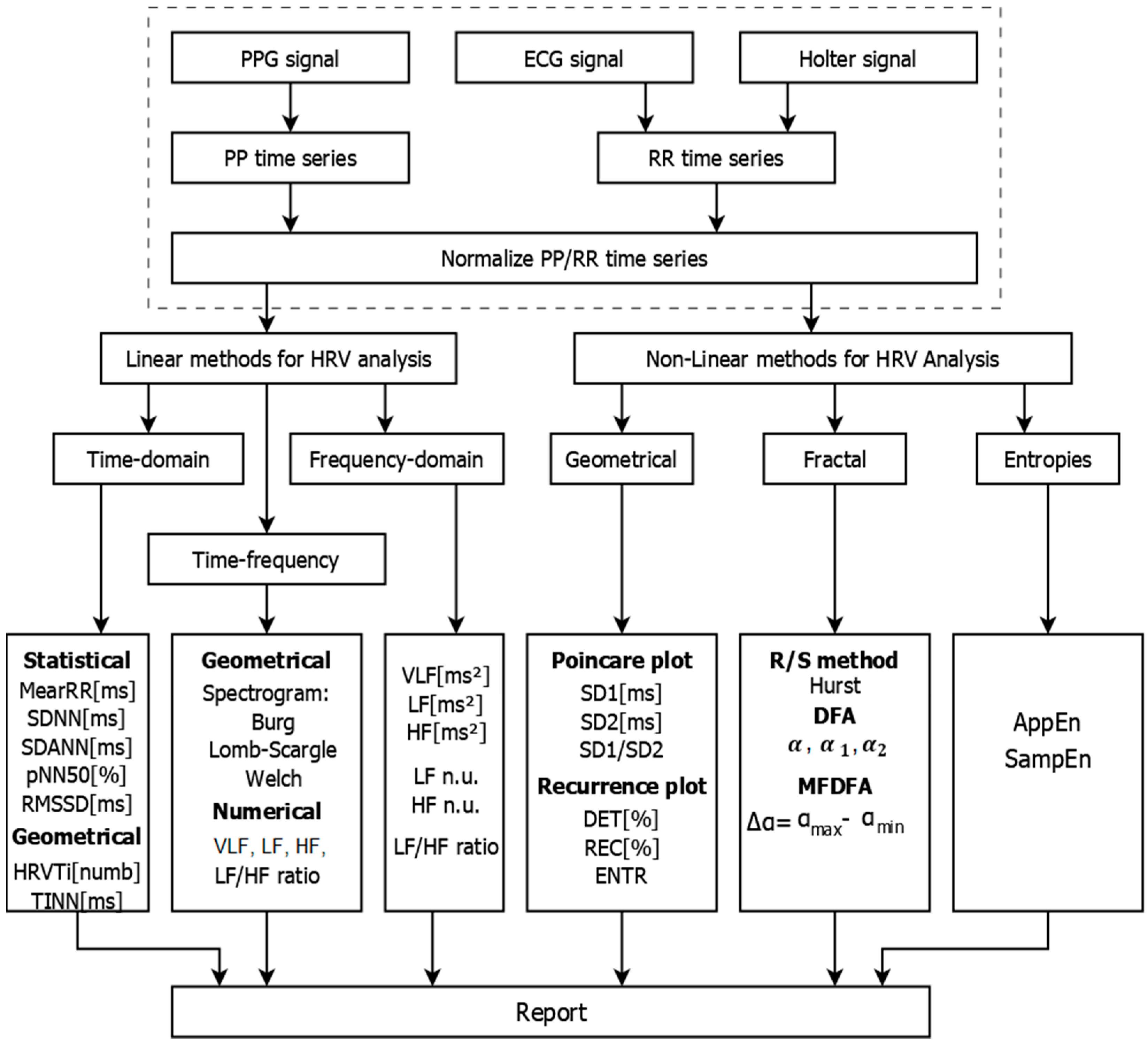
2.1. A Computer System for Analysis and Evaluation of HRV
- Cardiology registration via ECG, PPG and Holter devices and receipt of PP/RR time series;
- Mathematical analysis of the recorded data by applying linear and nonlinear methods. The results of the analysis are presented in tabular and graphical form;
- Creating a Report based on the results obtained, which can be stored in the patient database for later review and/or printing. In addition to the patient data, the database contains graphical information obtained through the graphical methods of analysis of HRV characteristics of various cardiovascular diseases.
- Linear methods: Time-Domain, Frequency-Domain, and Time-Frequency analysis;
- Nonlinear methods: Poincaré plot, Recurrence plot, Hurst R/S method, DFA, Multi-Fractal DFA, AppEn and SampEn.
2.2. Linear Methods for HRV Analysis
2.2.1. Time-Domain Analysis
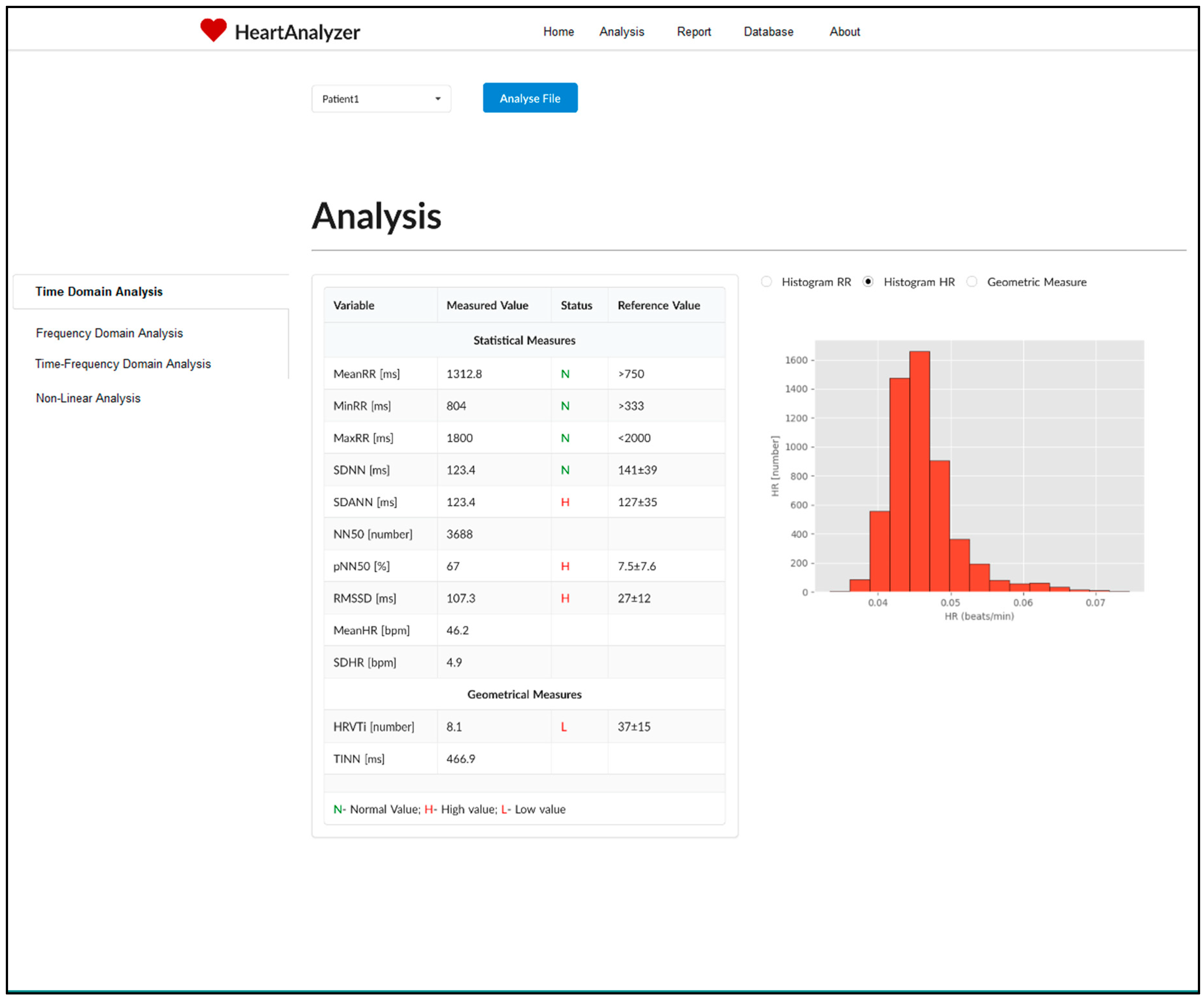
- SDNN (ms)—this parameter calculates the standard deviation from the average duration of RR intervals over the entire study period. It is used to evaluate total HRV and especially its parasympathetic component. The longer the study lasts, the more total HRV accumulates, so it is necessary that the compared signals have the same duration;
- SDANN (ms)—it defines the standard deviation from the average length of RR intervals by calculating the 5-minute segments. The registration period is split when a 24-hour ECG recording is used. This parameter is used to evaluate the low frequency components of HRV;
- SDNN index—determines the average of standard deviations from the average duration of RR intervals for all 5-minute periods divided by the observation period;
- RMSSD (ms)—determines the root mean square difference between the duration of adjacent RR intervals. This parameter reflects the fast, high frequency variability changes;
- NN50—the number of the pairs of consecutive NN intervals differing by more than 50 ms obtained over the entire recording period;
- pNN50—the percentage of consecutive intervals that differ by more than 50 ms. Because this parameter is determined by adjacent intervals, it reflects fast, high frequency variability changes.
- TINN—the distribution of RR intervals is approximated to a triangle and its base is measured in milliseconds. The essence of the algorithm is the following: the histogram is conventionally represented as a triangle, the base of the triangle is calculated by the formula: b = 2A/h, where h is the largest number of RR intervals, and A is the area of the whole histogram, i.e., the total number of all RR intervals analysed. This parameter avoids taking into account the RR intervals associated with artifacts and extrasystoles that form additional peaks and domes of the histogram;
- HRV triangular index—this parameter plot a histogram of RR intervals at 7.8125 ms (1/128 s). The total number of RR intervals is divided by the peak height of the histogram. This index reflects total HRV and is directly proportional to parasympathetic activity.
2.2.2. Frequency-Domain Analysis
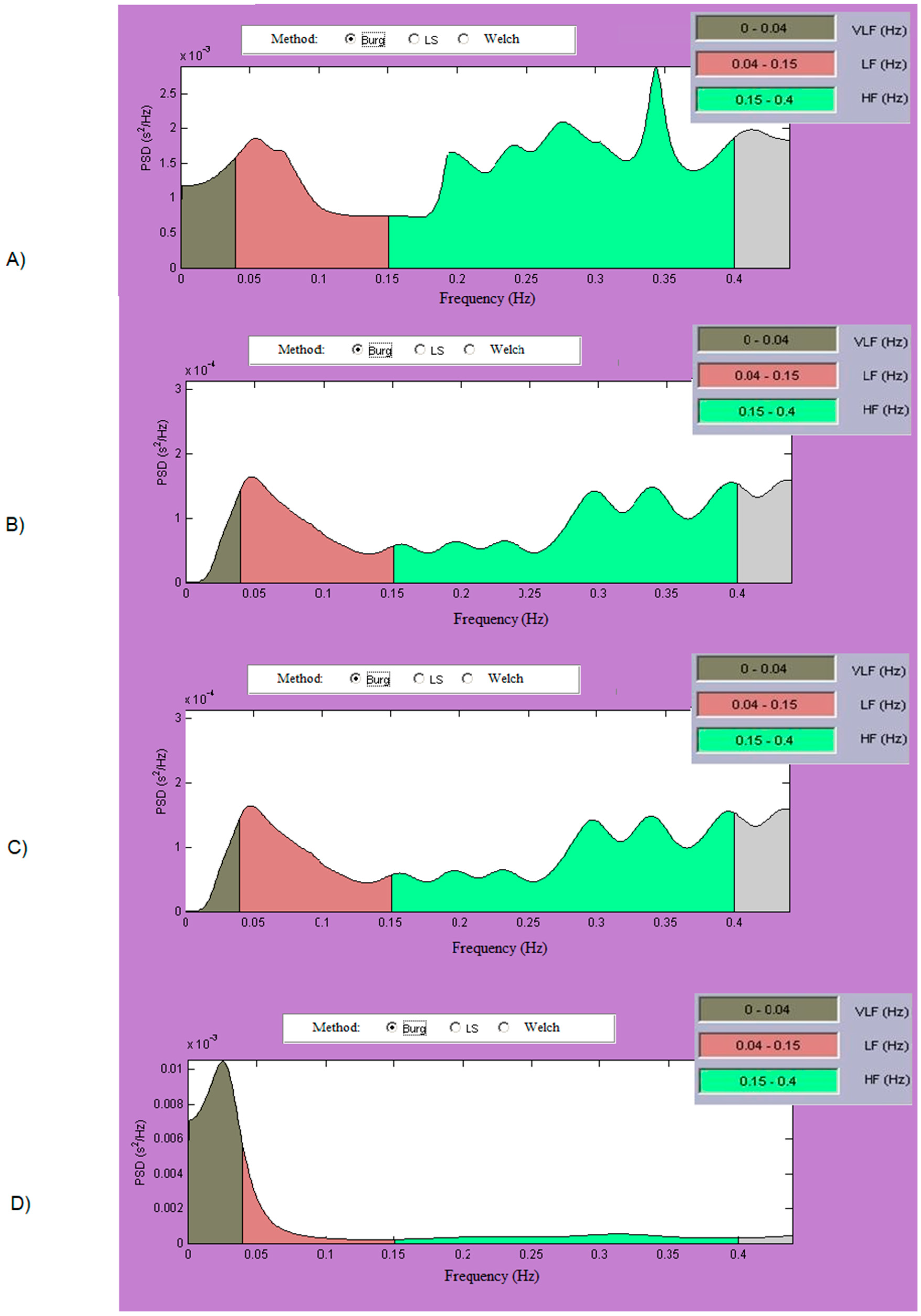
- Very low frequency—VLF: from 0.003 Hz to 0.04 Hz;
- Low frequency—LF: from 0.04 Hz to 0.15 Hz;
- High frequency—HF: from 0.15 Hz to 0.4 Hz.
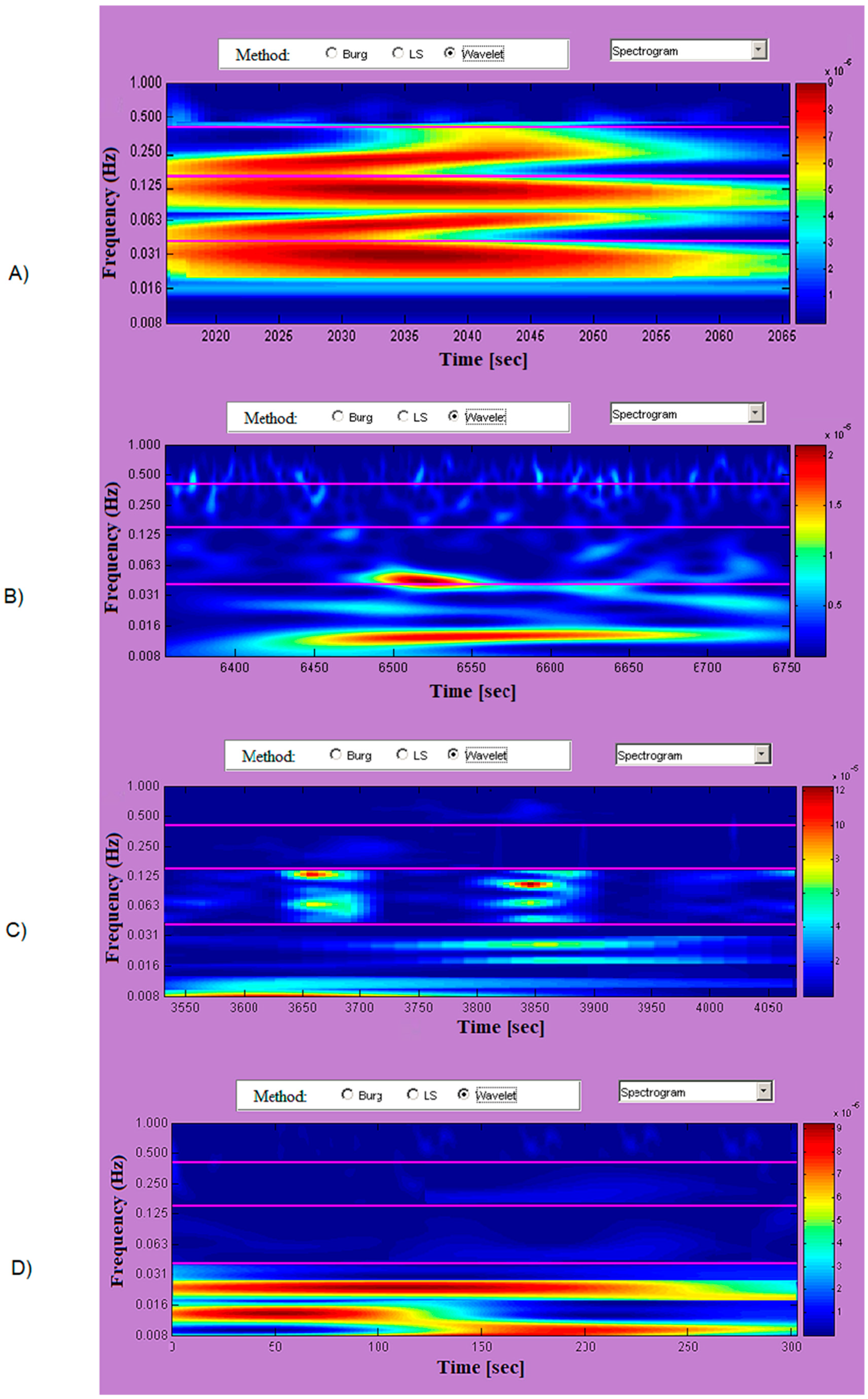
2.2.3. Time-Frequency Analysis
- Burg method—this method uses an autoregressive model of a different order, spline interpolation, Heming window, and window overlap apply;
- LombScargle method—the method calculates a non-normalized Lomb–Scargle periodogram;
- Wavelet method—based on the application of wavelet theory methods; applies wavelet interpolation of the investigated data, uses different wavelet bases (Morlet, Dobeshi, bi-orthogonal wavelets, and other wavelet bases) and calculates a continuous wavelet spectrum.
2.3. Nonlinear Methods for HRV Analysis
2.3.1. Geometric Nonlinear Methods
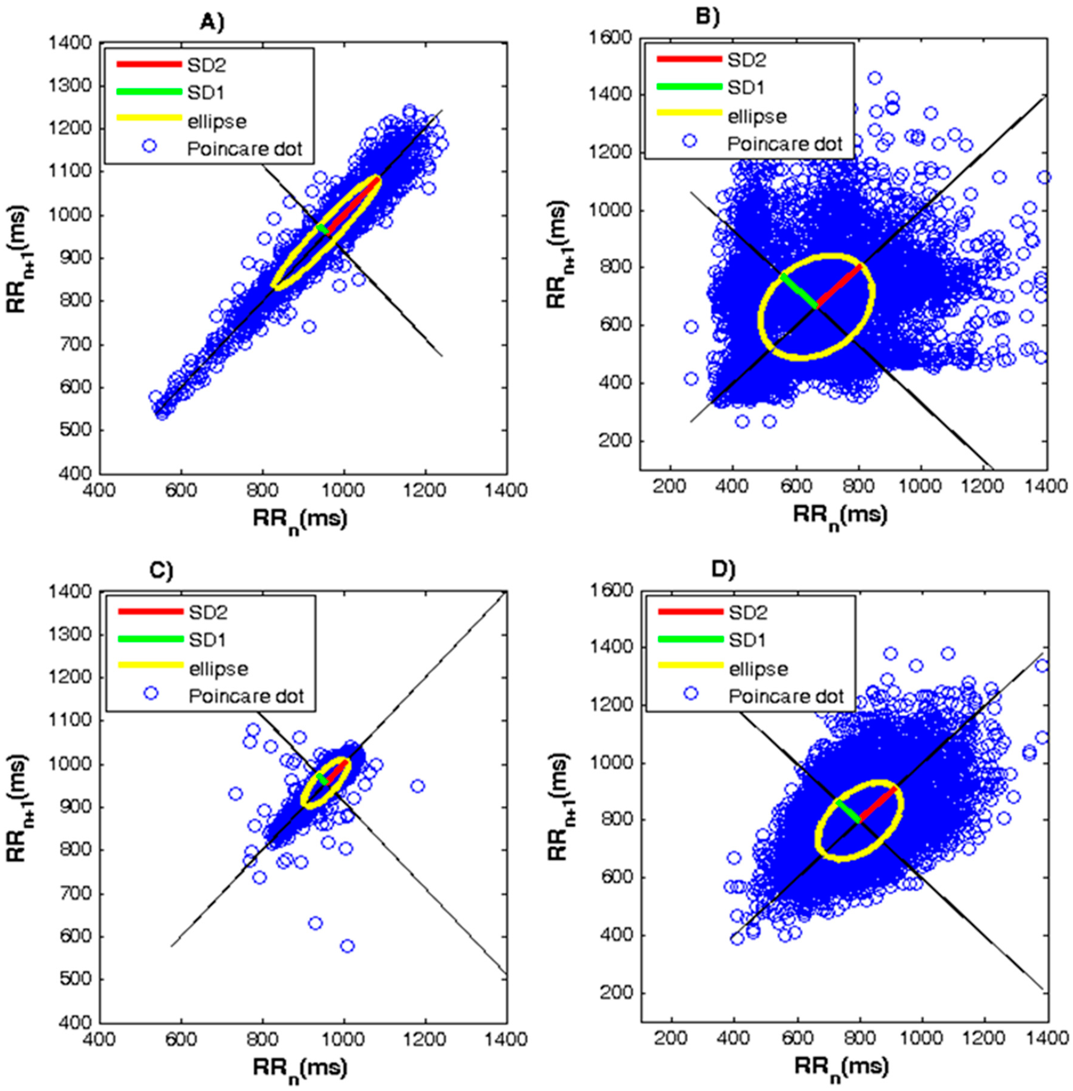
- Ellipse length (SD2 [ms] parameter)—corresponds to long-term variability of RR intervals and reflects total HRV;
- Ellipse Width (SD1 [ms] parameter)—represents the scattering of the dots perpendicular to the identity line and is associated with rapid variations between heart beats;
- The SD1/SD2 ratio reflects the relationship between short- and long-term HRV.
- The healthy subject’s graph has one major segment of points, which has the shape of a comet with a narrow bottom and gradually expanding to the top;
- The chart of the sick subject has the form of a torpedo, a fan or a complex form (consisting of several segments) depending on the type of disease.
- The graphic of a healthy subject has a clear ellipse;
- If the graph looks like a compressed segment of dots, then the narrow "compressed" ellipse means low HRV and is an indicator of a disease state;
- If the length and width of the ellipse are approximately equal and it approaches a circle, in this case, the HRV is low, which is an indicator of the disease state;
- If the points in the graph are symmetrical relative to the identity line, then there is no rhythm disturbance;
- If the points in the graph are asymmetric relative to the identity line, then the patient has rhythmic disturbances.
- Homogeneous processes with independent random values;
- Processes with slowly changing parameters;
- Periodic or oscillating processes, etc.
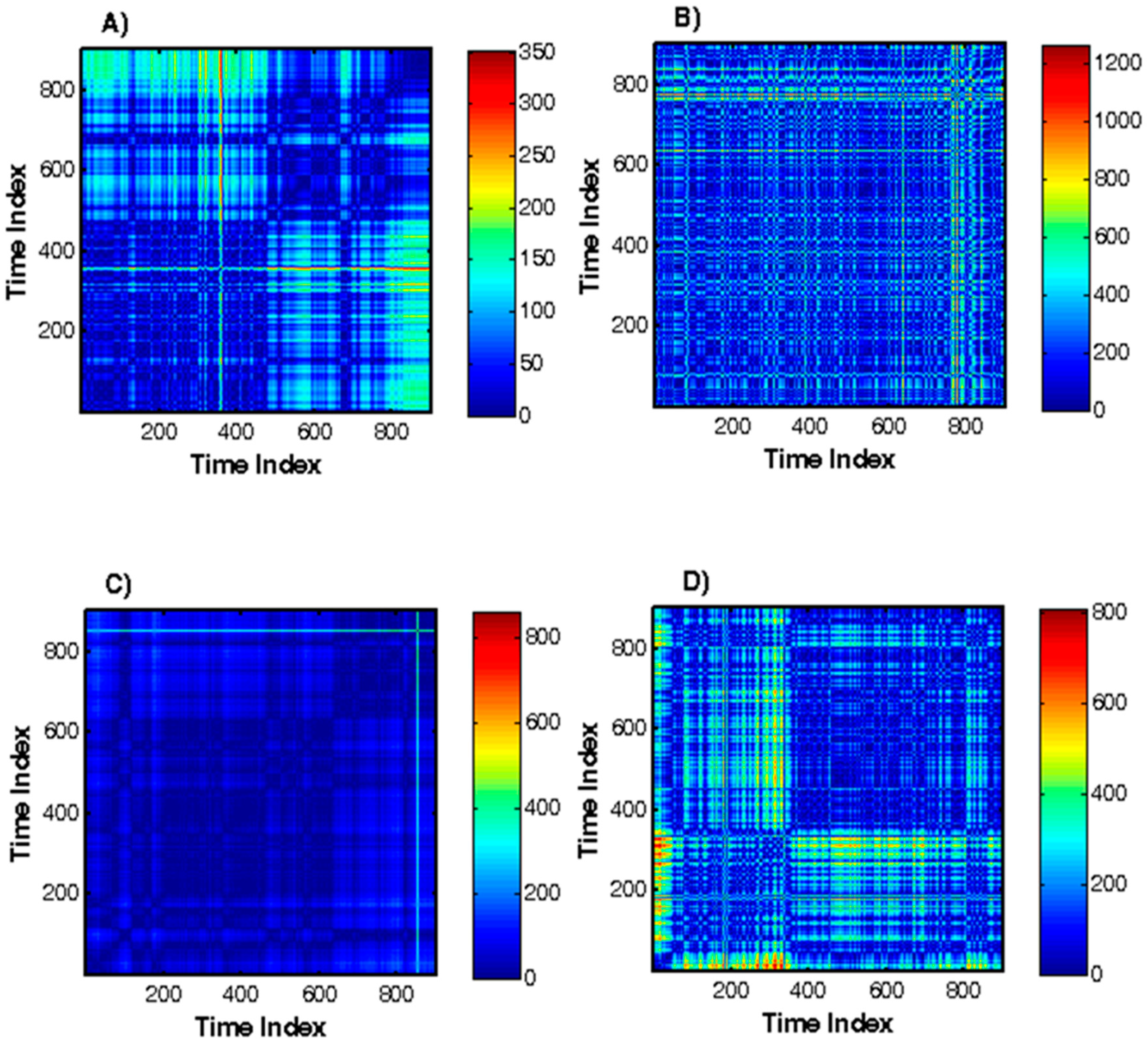
- Recurrence rate (REC%)—this parameter reflects the level of recurrence, indicating the probability of finding a recurring point in the RR series, that is, determining the probability of a recurrence of the condition. This variable ranges from 0% to 100%.
- Determinism (DET%)—this parameter is a characteristic of the predictability of the system. It is defined as the ratio between the number of recurrent points located on diagonal lines and the total number of recurrent points.
- ENTR—this parameter is related to Shannon entropy.
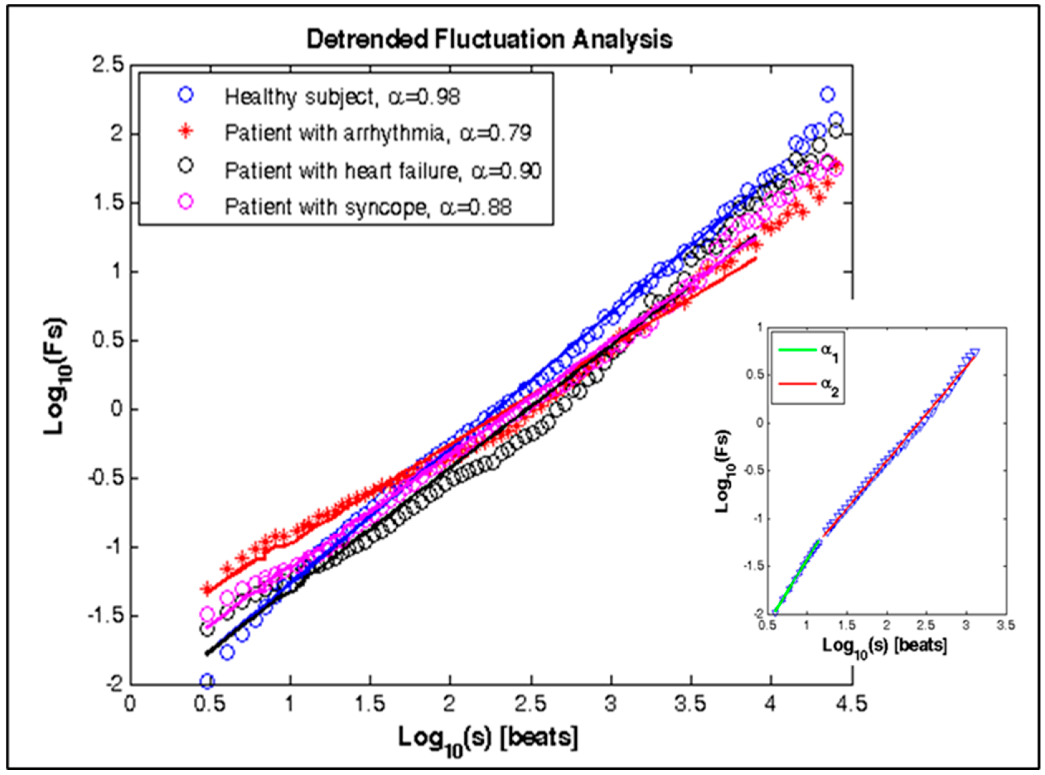
2.3.2. Fractal Methods
- β0—the point at which the regression line intersects the ordinate;
- β1—the slope of the regression line.
- H = α if 0< α <1;
- H = α-1 if α ≥ 1.
2.3.3. Entropies Methods
2.4. Data Collection
2.5. Statistical Analysis
3. Results
3.1. Linear Methods for HRV Analysis
3.2. Nonlinear Methods for HRV Analysis
4. Discussion
4.1. Linear Analysis
4.2. Nonlinear Analysis
5. Limitations
6. Conclusions
Author Contributions
Funding
Conflicts of Interest
References
- Shaffer, F.; Ginsberg, J.P. An Overview of Heart Rate Variability Metrics and Norms. Front. Public Health 2017, 5, 258. [Google Scholar] [CrossRef] [PubMed] [Green Version]
- Reed, M.J.; Robertson, C.E.; Addison, P.S. Heart rate variability measurements and the prediction of ventricular arrhythmias. QJM Int. J. Med. 2005, 98, 87–95. [Google Scholar] [CrossRef] [PubMed] [Green Version]
- Elgendi, M.; Norton, I.; Brearley, M.; Dokos, D.; Abbott, D.; Schuurmans, D. A pilot study: Can heart rate variability (HRV) be determined using short-term photoplethysmograms? F1000Research 2016, 5, 2354. [Google Scholar] [CrossRef] [Green Version]
- Evans, S.; Seidman, L.C.; Tsao, J.C.; Lung, K.C.; Zeltzer, L.K.; Naliboff, B.D. Heart rate variability as a biomarker for autonomic nervous system response differences between children with chronic pain and healthy control children. J. Pain Res. 2013, 6, 449–457. [Google Scholar] [CrossRef] [Green Version]
- Deldar, K.; Bahaadinbeigy, K.; Tara, S.M. Teleconsultation and Clinical Decision Making: A Systematic Review. Acta Inform. Med. 2016, 24, 286–292. [Google Scholar] [CrossRef] [Green Version]
- Jan, H.; Chen, M.; Fu, T.; Lin, W.; Tsai, C.; Lin, K. Evaluation of Coherence Between ECG and PPG Derived Parameters on Heart Rate Variability and Respiration in Healthy Volunteers With/Without Controlled Breathing. J. Med. Biol. Eng. 2019, 39, 783–795. [Google Scholar] [CrossRef] [Green Version]
- Reynders, T.; Gidron, Y.; De Ville, J.; Bjerke, M.; Weets, I.; Van Remoortel, A.; Devolder, L.; D’haeseleer, M.; De Keyser, J.; Nagels, G.; et al. Relation between Heart Rate Variability and Disease Course in Multiple Sclerosis. J. Clin. Med. 2020, 9, 3. [Google Scholar] [CrossRef] [Green Version]
- Kim, H.; Ishag, M.; Piao, M.; Kwon, T.; Ryu, K. A Data Mining Approach for Cardiovascular Disease Diagnosis Using Heart Rate Variability and Images of Carotid Arteries. Symmetry 2016, 8, 47. [Google Scholar] [CrossRef] [Green Version]
- Park, H.; Dong, S.Y.; Youm, M. The Role of Heart-Rate Variability Parameters in Activity Recognition and Energy-Expenditure Estimation Using Wearable Sensors. Sensors 2017, 17, 1698. [Google Scholar] [CrossRef]
- Acharya, U.R.; Ghista, D.; Yi, Z.; Min, L.; Ng, E.; Sree, S.; Faust, O.; Weidong, L.; Alvin, A. Integrated index for cardiac arrythmias diagnosis using entropies as features of heart rate variability signal. In Proceedings of the 2011 1st Middle East. Conference on Biomedical Engineering, Sharjah, UAE, 21–24 February 2011; pp. 371–374. [Google Scholar] [CrossRef]
- Inan, O.T.; Giovangrandi, L.; Kovacs, G.T.A. Robust neural-network based classification of premature ventricular contractions using wavelet transform and timing interval features. IEEE Trans. Biomed. Eng. 2006, 53, 2507–2515. [Google Scholar] [CrossRef]
- Faust, O.; Ng, E. Computer aided diagnosis for cardiovascular diseases based on ECG signals: A survey. J. Mech. Med. Biol. 2016, 16, 1640001. [Google Scholar] [CrossRef]
- Wei, H.-C.; Ta, N.; Hu, W.-R.; Wang, S.-Y.; Xiao, M.-X.; Tang, X.-J.; Chen, J.-J.; Wu, H.-T. Percussion Entropy Analysis of Synchronized ECG and PPG Signals as a Prognostic Indicator for Future Peripheral Neuropathy in Type 2 Diabetic Subjects. Diagnostics 2020, 10, 32. [Google Scholar] [CrossRef] [PubMed] [Green Version]
- Onchis, D.; Istin, C.; Tudoran, C.; Tudoran, M.; Real, P. Timely-Automatic Procedure for Estimating the Endocardial Limits of the Left Ventricle Assessed Echocardiographically in Clinical Practice. Diagnostics 2020, 10, 40. [Google Scholar] [CrossRef] [PubMed] [Green Version]
- Yamashita, Y.; Tanioka, K.; Kawaji, Y.; Tamura, T.; Nuta, J.; Hatamaru, K.; Itonaga, M.; Yoshida, T.; Ida, Y.; Maekita, T.; et al. Utility of Contrast-Enhanced Harmonic Endoscopic Ultrasonography for Early Diagnosis of Small Pancreatic Cancer. Diagnostics 2020, 10, 23. [Google Scholar] [CrossRef] [Green Version]
- Kubios (version 3.3). User’s Guide. 2019. Available online: https://www.kubios.com/downloads/Kubios_HRV_Users_Guide.pdf (accessed on 5 June 2019).
- Mourot, L. CODESNA_HRV, a new tool to assess the activity of the autonomic nervous system from heart rate variability. Phys. Med. Rehabil. Res. 2018, 3, 1–6. [Google Scholar] [CrossRef] [Green Version]
- Perakakis, P.; Joffily, M.; Taylor, M.; Guerraa, P.; Vila, J. KARDIA: A Matlab software for the analysis of cardiac interbeat intervals. Comput. Methods Programs Biomed. 2010, 98, 83–89. [Google Scholar] [CrossRef]
- Bartels, R.; Neumamm, L.; Pecanha, T.; Carvalho, S. SinusCor: An advanced tool for heart rate variability analysis. BioMed. Eng. 2017, 16, 110–124. [Google Scholar] [CrossRef]
- Pichot, V.; Roche, F.; Celle, S.; Barthélémy, J.C.; Chouchou, F. HRV analysis: A Free Software for Analyzing Cardiac Autonomic Activity. Front. Physiol. 2016, 7, 557. [Google Scholar] [CrossRef]
- Rodrίguez-Liñres, L.; Lado, M.J.; Vila, X.A.; Méndz, A.J.; Guesta, P. gHRV: Heart Rate Variability analysis made easy. Comput. Methods Programs Biomed. 2014, 116, 26–38. [Google Scholar] [CrossRef]
- García Martínez, C.A.; Otero Quintana, A.; Vila, X.A.; Lado Touriño, M.J.; Rodríguez-Liñares, L.; Rodríguez Presedo, J.M.; Méndez Penín, A.J. HRV Analysis with the R package RHRV; Springer International Publishing AG: Cham, Switzerland, 2017. [Google Scholar] [CrossRef]
- Malik, M. Task Force of the European Society of Cardiology and the North American Society of Pacing and Electrophysiology, heart rate variability—Standards of measurement, physiological interpretation, and clinical use. Circulation 1996, 93, 1043–1065. [Google Scholar] [CrossRef] [Green Version]
- Ernst, G. Heart Rate Variability; Springer: London, UK, 2014. [Google Scholar]
- Welch, P. The use of fast Fourier transform for the estimation of power spectra: A method based on time averaging over short, modified periodograms. IEEE Trans. Audio Electroacoust. 1967, 15, 70–73. Available online: https://pdfs.semanticscholar.org/e633/45b4243e2376720a4e66373fdffe7a7d6be0.pdf (accessed on 12 March 2020). [CrossRef] [Green Version]
- Goldberger, A.; Rigney, D.; West, B. Science in Pictures: Chaos and Fractals in Human Physiology. Sci. Am. 1990, 262, 42–49. Available online: https://www.scientificamerican.com/article/science-in-pictures-chaos-and-fract/ (accessed on 12 March 2020). [CrossRef] [PubMed]
- Peng, C.-K.; Havlin, S.; Stanley, H.E.; Goldberger, A.L. Quantification of Scaling Exponents and Crossover Phenomena in Nonstationary Heartbeat Time Series. CHAOS 1995, 5, 82–87. [Google Scholar] [CrossRef] [PubMed]
- Tayel, M.B.; AlSaba, E.I. Poincaré Plot for Heart Rate Variability. Int. J. Biomed. Biol. Eng. 2015, 9, 708–711. [Google Scholar] [CrossRef]
- Khandoker, A.H.; Karmakar, G.; Brennan, M.; Voss, A.; Palaniswami, M. Poincare Plot Methods for Heart Rate Variability Analysis; Springer: Berlin/Heidelberg, Germany, 2013. [Google Scholar]
- Marwan, N.; Romano, M.C.; Thiel, M.; Kurths, J. Recurrence plots for the analysis of complex systems. Phys. Rep. 2007, 438, 237–329. [Google Scholar] [CrossRef]
- Acharya, U.R.; Faust, O.; Dhanjoo, N.; Ghista, S.; Sree, V.; Alvin, A.; Chattopadhyay, S.; Lim, Y.; Ng, E.; Yu, W. A Systems Approach to Cardiac Health Diagnosis. J. Med Imaging Health Inform. 2013, 3, 1–7. [Google Scholar] [CrossRef]
- Acharya, U.R.; Suri, J.S.; Spaan, J.A.E.; Krishnan, S.M. Advances in Cardiac Signal. Processing; Springer: Berlin/Heidelberg, Germany, 2007. [Google Scholar]
- Bhavsar, R.; Davey, N.; Helian, N.; Sun, Y.; Steffert, T.; Mayor, D. Time Series Analysis using Embedding Dimension on Heart Rate Variability. Procedia Comput. Sci. 2018, 145, 89–96. [Google Scholar] [CrossRef]
- Nayak, S.K.; Bit, A.; Dey, A.; Mohapatra, B.; Pa, K. A Review on the Nonlinear Dynamics System Analysis of Electrocardiogram Signal. J. Healthc. Eng. 2018, 6920420. [Google Scholar] [CrossRef] [Green Version]
- Tsuji, S.; Aihara, K. Criterion for determining the optimal delay of attractor reconstruction using persistent homology. Nonlinear Theory Appl. IEICE 2019, 10, 74–89. [Google Scholar] [CrossRef]
- Guler, N.F.; Ubeyly, E.D.; Guler, I. Recurrent neural networks employing Lyapunov exponents for RRG signals classification. Expert Syst. Appl. 2005, 29, 506–514. [Google Scholar] [CrossRef]
- Rosenstein, M.T.; Collins, J.J.; Luca, C.J. A practical method for calculating largest Lyapunov exponents from small data sets. In NeuroMuscular Research Center and Department of Biomedical Engineering; Boston University: Boston, MA, USA, 1992; Available online: https://archive.physionet.org/physiotools/lyapunov/RosensteinM93.pdf (accessed on 12 March 2020).
- Kale, M.; Butar, F.B. Fractal analysis of Time Series and Distribution Properties of Hurst Exponent. J. Math. Sci. Math. Educ. 2011, 5, 8–19. Available online: http://msme.us/2011-1-2.pdf (accessed on 12 March 2020).
- Sheluhin, O.I.; Smolskiy, S.M.; Osin, A.V. Self-Similar Processes in Telecommunications; John Wiley & Sons, Ltd.: Chichester, UK, 2007. [Google Scholar]
- Mandelbrot, B. Fractals and Scaling in Finance; Springer: New York, NY, USA, 1997. [Google Scholar]
- Mulligan, R. Fractal analysis of highly volatile markets: An application to technology equities. Q. Rev. Econ. Financ. 2004, 44, 155–179. Available online: https://ideas.repec.org/a/eee/quaeco/v44y2004i1p155-179.html (accessed on 12 March 2020). [CrossRef]
- Golińska, A.K. Detrended Fluctuation Analysis (DFA) in Biomedical Signal Processing: Selected Examples. Stud. Logic Gramm. Rhetor. 2012, 29, 107–115. Available online: https://philpapers.org/rec/KITDFA (accessed on 12 March 2020).
- Maraun, D.; Rust, H.W.; Timmer, J. Tempting long-memory—On the interpretation of DFA results. Nonlinear Process. Geophys. Eur. Geosci. Union (EGU) 2004, 11, 495–503. [Google Scholar] [CrossRef] [Green Version]
- Kantelhardt, J.W.; Zschiegner, S.A.; Koscielny-Bunde, E.; Havlin, S.; Bunde, A.; Stanley, H.E. Multifractal detrended fluctuation analysis of nonstationary time series. Phys. A Stat. Mech. Appl. 2002, 316, 87–114. [Google Scholar] [CrossRef] [Green Version]
- Biswas, A.; Zeleke, T.B.; Si, B.C. Multifractal detrended fluctuation analysis in examining scaling properties of the spatial patterns of soil water storage. Nonlinear Process. Geophys. 2012, 19, 227–238. [Google Scholar] [CrossRef] [Green Version]
- Li, E.; Mu, X.; Zhao, G.; Gao, P. Multifractal Detrended Fluctuation Analysis of Streamflow in the Yellow River Bain, China. Water 2015, 7, 1670–1686. [Google Scholar] [CrossRef] [Green Version]
- Kalisky, T.; Ashkenazy, Y.; Havlin, S. Volatility of fractal and multifractal time series. Isr. J. Earth Sci. 2007, 65, 47–56. [Google Scholar] [CrossRef] [Green Version]
- Al-Angari, H.M.; Sahakian, A.V. Use of Sample Entropy Approach to Study Heart Rate Variability in Obstructive Sleep Apnea Syndrome. IEEE Trans. Biomed. Eng. 2007, 54, 1900–1904. [Google Scholar] [CrossRef]


| Parameter | Group 1 (mean ± SD) n = 48 | Group 2 (mean ± SD) n = 56 | Group 3 (mean ± SD) n = 59 | Group 4 (mean ± SD) n = 49 | Statistical p-Value | ||
|---|---|---|---|---|---|---|---|
| Gr1,2 | Gr1,3 | Gr1,4 | |||||
| Statistical measurement | |||||||
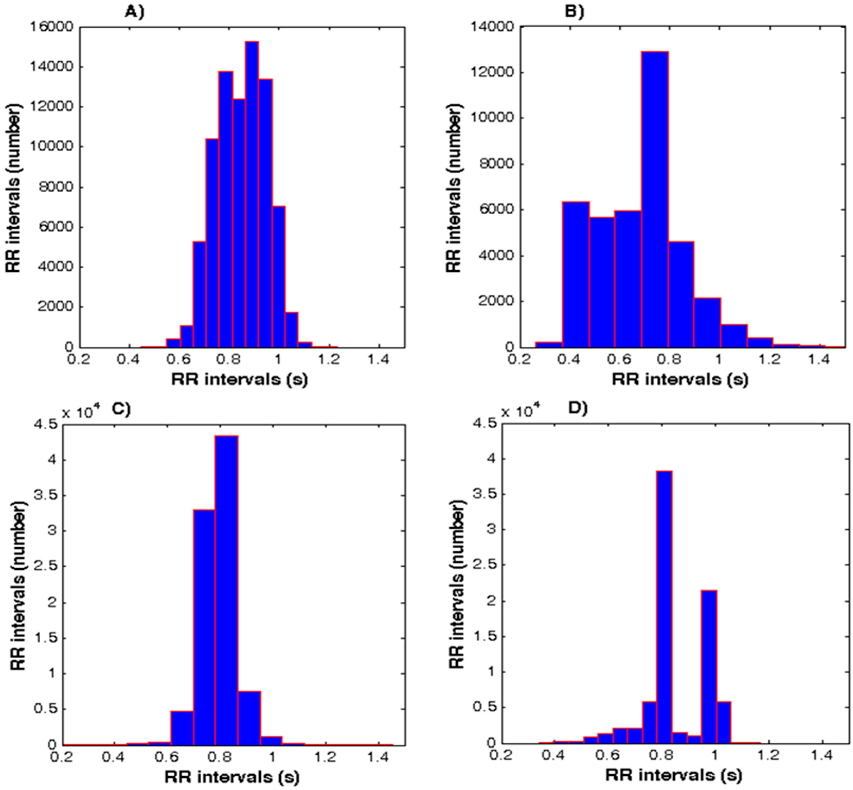
| MeanRR [ms] | 849 ± 28 | 679 ± 18 | 880 ± 20 | 855 ± 35 | 0.0001 | 0.0005 | 0.0001 |
| SDNN [ms] | 121.8 ± 21 | 62 ± 15 | 72 ± 18 | 60 ± 15 | 0.0001 | 0.0001 | 0.0001 |
| SDANN [ms] | 140 ± 15 | 64 ± 10 | 70 ± 12 | 28 ± 4 | 0.0001 | 0.0001 | 0.0001 |
| pNN50 [%] | 14.8 ± 3 | 13 ± 5 | 9.1 ± 2 | 6.7 ± 1 | 0.03 | 0.0001 | 0.0001 |
| RMSSD [ms] | 25.8 ± 9 | 17 ± 2 | 16 ± 3 | 12 ± 5 | 0.0001 | 0.0001 | 0.0001 |
| Geometrical measurement | |||||||
| HRVti [numb] | 21.8 ± 10 | 6.2 ± 2.7 | 1.5 ± 1.2 | 3.1 ± 1.6 | 0.0001 | 0.0001 | 0.0001 |
| TINN [ms] | 493 ± 80 | 542 ± 70 | 381 ± 60 | 52 ± 11 | 0.002 | 0.0001 | 0.0001 |
| Parameter | Group 1 (mean ± SD) n = 48 | Group 2 (mean ± SD) n = 56 | Group 3 (mean ± SD) n = 59 | Group 4 (mean ± SD) n = 49 | Statistical p-Value | ||
|---|---|---|---|---|---|---|---|
| Gr1,2 | Gr1,3 | Gr1,4 | |||||
| VLF Power [ms2] | 13226.42 ± 674.12 | 12602.93 ±984.17 | 11939.57 ± 489.73 | 17846.84 ± 692.41 | 0.0004 | 0.0001 | 0.0001 |
| LF Power [ms2] | 1198.88 ± 562.93 | 549.98 ± 181.42 | 411.82 ± 247.79 | 486.26 ± 164.33 | 0.0001 | 0.0007 | 0.0001 |
| HF Power [ms2] | 791.03 ±243.18 | 675.71 ± 269.14 | 301.93 ± 354.81 | 534.35 ± 388.96 | 0.0234 | 0.002 | 0.0002 |
| LF Power nu | 0.602 ± 0.23 | 0.449 ± 0.11 | 0.577 ± 0.19 | 0.476 ± 0.21 | 0.0001 | NS * (0.5393) | 0.0059 |
| HF Power nu | 0.398 ± 0.19 | 0.551 ± 0.13 | 0.423 ± 0.08 | 0.524 ± 0.195 | 0.0001 | NS * (0.3615) | 0.0018 |
| LF/HF | 1.52 ± 0.57 | 0.81 ± 0.22 | 1.36 ± 0.07 | 0.91 ± 0.68 | 0.0001 | 0.0475 | 0.0001 |
| Parameter | Group 1 (mean ± SD) n = 48 | Group 2 (mean ± SD) n = 56 | Group 3 (mean ± SD) n = 59 | Group 4 (mean ± SD) n = 49 | Statistical p-Value | ||
|---|---|---|---|---|---|---|---|
| Gr1,2 | Gr1,3 | Gr1,4 | |||||
| Poincaré plot | |||||||
| SD1 [ms] | 61.2 ± 10.3 | 55.5 ± 12.8 | 49.8 ± 9.9 | 45.1 ± 11.0 | 0.014 | 0.0001 | 0.0001 |
| SD2 [ms] | 218.1 ± 26.2 | 73.3 ± 10.5 | 106.2 ± 11.9 | 96.1 ± 9.2 | 0.0001 | 0.0001 | 0.0001 |
| SD1/SD2 | 0.31 ± 0.7 | 0.87 ± 0.11 | 0.54 ± 0.2 | 0.52 ± 0.12 | 0.0001 | 0.0001 | 0.0001 |
| Recurrence plot | |||||||
| DET [%] | 90.8 ± 0.11 | 97.9 ± 0.13 | 99.06 ± 0.09 | 98.8 ± 0.1 | 0.0001 | 0.0001 | 0.0001 |
| REC [%] | 36.3 ± 0.2 | 43.4 ± 0.5 | 41.1 ± 0.3 | 39.5 ± 0.3 | 0.0001 | 0.0001 | 0.0001 |
| Lmax [beats] | 58 ± 12 | 136 ± 22 | 305 ± 31 | 104 ± 11 | 0.0001 | 0.0001 | 0.0001 |
| ENTR | 3.20 ± 0.3 | 3.48 ± 0.4 | 4.12 ± 0.1 | 3.80 ± 0.3 | 0.0001 | 0.0001 | 0.0001 |
| R/S method | |||||||
| Hurst | 0.98 ± 0.07 | 0.95 ± 0.04 | 0.96 ± 0.05 | 0.94 ± 0.13 | 0.06 | 0.09 | 0.06 |
| Detrended Fluctuation Analysis | |||||||
| α | 0.98 ± 0.03 | 0.77 ± 0.05 | 0.86 ± 0.06 | 0.81 ± 0.07 | 0.0001 | 0.0001 | 0.0001 |
| α1 | 1.16 ± 0.04 | 0.79 ± 0.04 | 0.89 ± 0.05 | 0.82 ± 0.06 | 0.0001 | 0.0001 | 0.0001 |
| α2 | 0.91 ± 0.03 | 0.68 ± 0.03 | 0.75 ± 0.04 | 0.72 ± 0.04 | 0.0001 | 0.0001 | 0.0001 |
| Multi-Fractal Detrended Fluctuation Analysis | |||||||
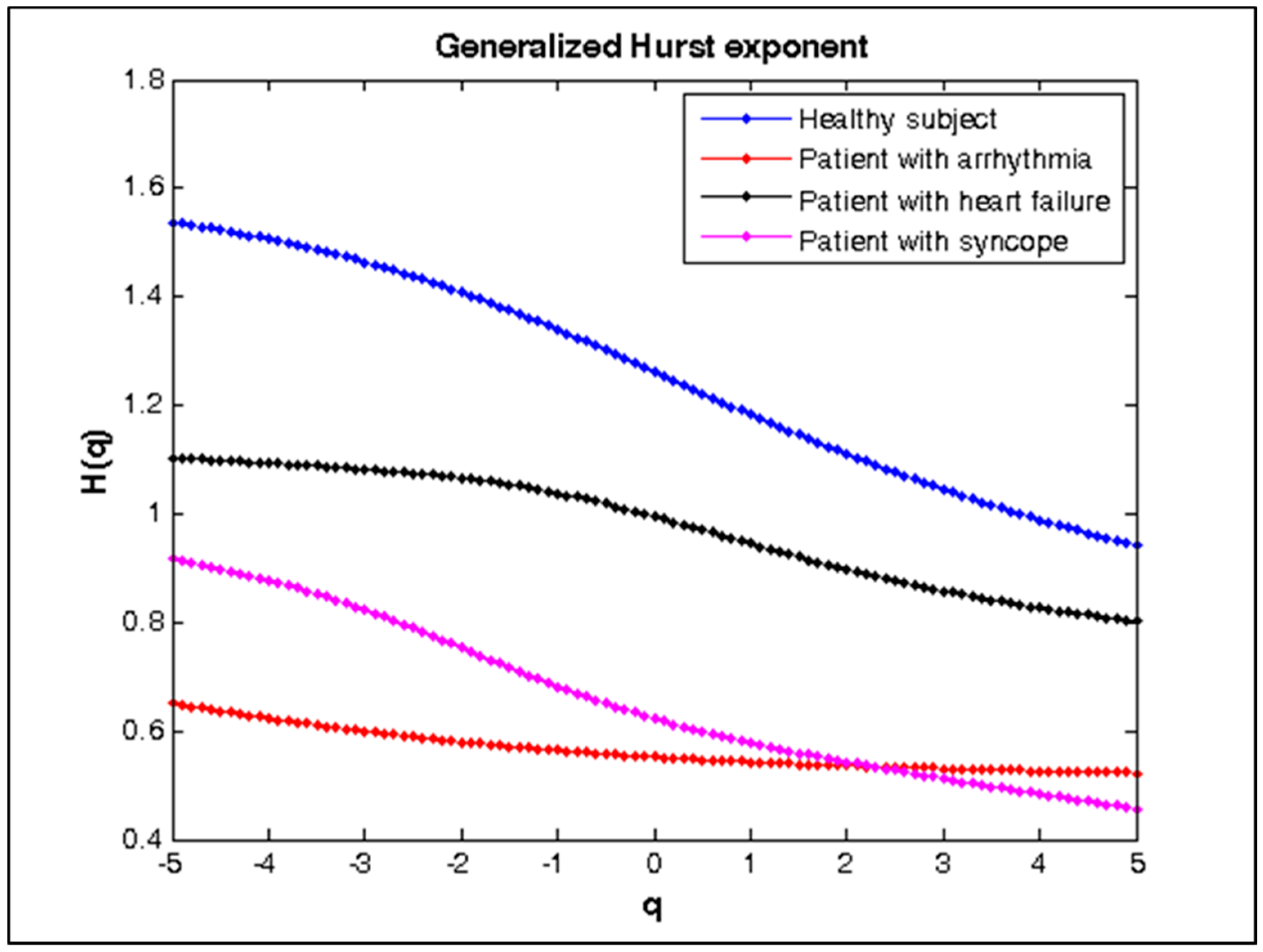
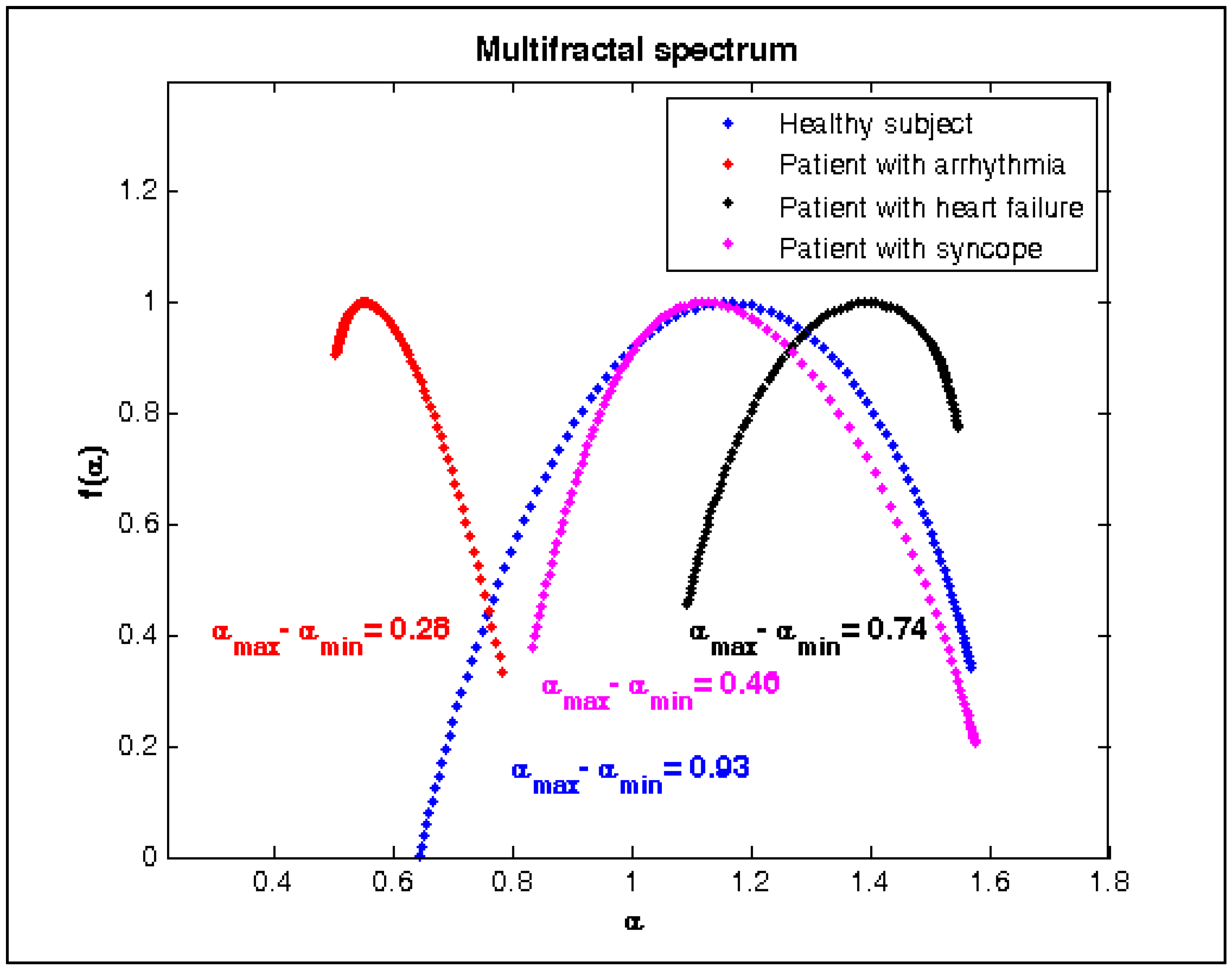
| Δα=αmax−αmin | 0.956 ± 0.05 | 0.281 ± 0.01 | 0.773 ± 0.03 | 0.494 ± 0.04 | 0.0001 | 0.0001 | 0.0001 |
| Entropies | |||||||
| AppEn | 1.57 ± 0.19 | 1.29 ± 0.25 | 1.08 | 1.32 | 0.0001 | 0.0001 | 0.0001 |
| SampEn | 1.53 ± 0.22 | 1.14 ± 0.21 | 1.17 | 1.25 | 0.0001 | 0.0001 | 0.0001 |
© 2020 by the authors. Licensee MDPI, Basel, Switzerland. This article is an open access article distributed under the terms and conditions of the Creative Commons Attribution (CC BY) license (http://creativecommons.org/licenses/by/4.0/).
Share and Cite
Georgieva-Tsaneva, G.; Gospodinova, E.; Gospodinov, M.; Cheshmedzhiev, K. Cardio-Diagnostic Assisting Computer System. Diagnostics 2020, 10, 322. https://doi.org/10.3390/diagnostics10050322
Georgieva-Tsaneva G, Gospodinova E, Gospodinov M, Cheshmedzhiev K. Cardio-Diagnostic Assisting Computer System. Diagnostics. 2020; 10(5):322. https://doi.org/10.3390/diagnostics10050322
Chicago/Turabian StyleGeorgieva-Tsaneva, Galya, Evgeniya Gospodinova, Mitko Gospodinov, and Krasimir Cheshmedzhiev. 2020. "Cardio-Diagnostic Assisting Computer System" Diagnostics 10, no. 5: 322. https://doi.org/10.3390/diagnostics10050322
APA StyleGeorgieva-Tsaneva, G., Gospodinova, E., Gospodinov, M., & Cheshmedzhiev, K. (2020). Cardio-Diagnostic Assisting Computer System. Diagnostics, 10(5), 322. https://doi.org/10.3390/diagnostics10050322