
Explainable Machine Learning Model for Glaucoma Diagnosis and Its Interpretation


Abstract
:1. Introduction
2. Materials and Methods
2.1. Participants
2.2. Prediction Model
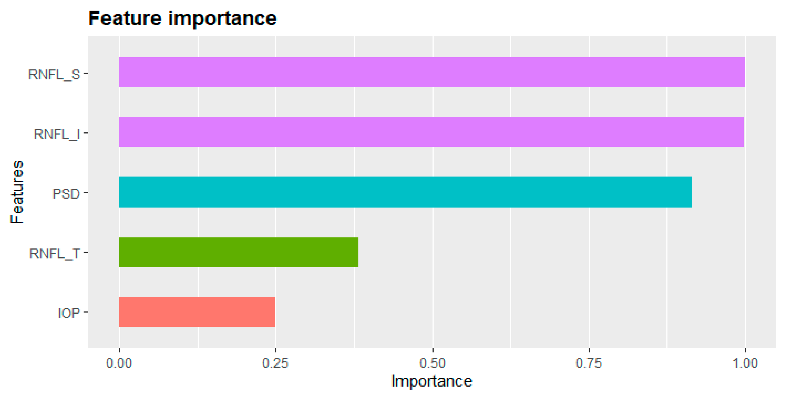
2.3. Explanations of an Individual Prediction
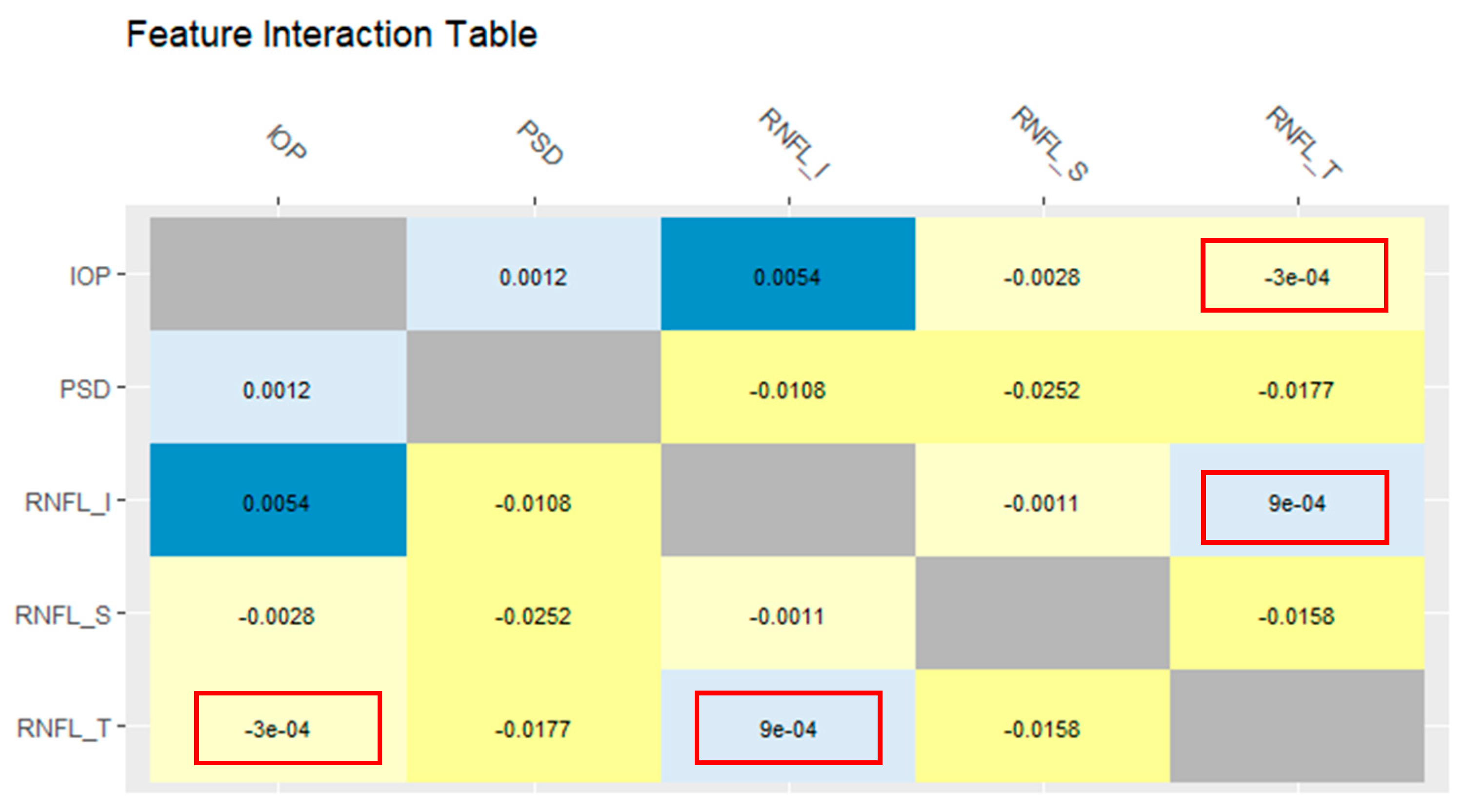
3. Results
4. Discussion
4.1. Diagnosis of Glaucoma
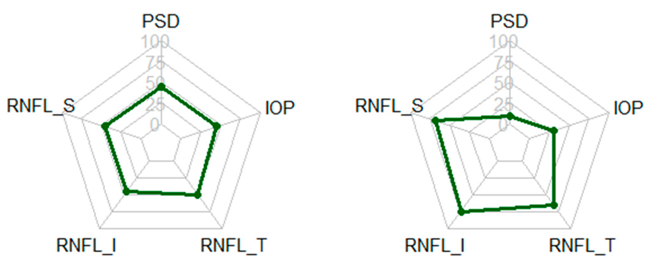
4.2. Case Analysis of Prediction Results
4.3. Analysis of Missed Predicted Cases
5. Conclusions
Supplementary Materials
Author Contributions
Funding
Institutional Review Board Statement
Informed Consent Statement
Data Availability Statement
Conflicts of Interest
References
- Shaikh, Y.; Yu, F.; Coleman, A.L. Burden of undetected and untreated glaucoma in the United States. Am. J. Ophthalmol. 2014, 158, 1121–1129.e1. [Google Scholar] [CrossRef] [PubMed]
- Taketani, Y.; Murata, H.; Fujino, Y.; Mayama, C.; Asaoka, R. How many visual felds are required to precisely predict future test results in glaucoma patients when using diferent trend analyses? Investig. Ophthalmol. Vis. Sci. 2015, 56, 4076–4082. [Google Scholar] [CrossRef] [PubMed] [Green Version]
- Asaoka, R.; Murata, H.; Iwase, A.; Araie, M. Detecting preperimetric glaucoma with standard automated perimetry using a deep learning classifer. Ophthalmology 2016, 123, 1974–1980. [Google Scholar] [CrossRef]
- An, G.; Omodaka, K.; Hashimoto, K.; Tsuda, S.; Shiga, Y.; Takada, N.; Kikawa, T.; Yokota, H.; Akiba, M.; Nakazawa, T. Glaucoma diagnosis with machine learning based on optical coherence tomography and color fundus images. J. Healthc. Eng. 2019, 1, 10. [Google Scholar] [CrossRef]
- Wang, P.; Shen, J.; Chang, R.; Moloney, M.; Torres, M.; Burkemper, B.; Jiang, X.; Rodger, D.; Varma, R.; Richter, G.M. Machine learning models for diagnosing glaucoma from retinal nerve fiber layer thickness maps. Ophthalmol. Glaucoma 2019, 2, 422–428. [Google Scholar] [CrossRef] [PubMed]
- Asaoka, R.; Murata, H.; Hirasawa, K.; Fujino, Y.; Matsuura, M.; Miki, A.; Kanamoto, T.; Ikeda, Y.; Mori, K.; Iwase, A.; et al. Using deep learning and transfer learning to accurately diagnose early-onset glaucoma from macular optical coherence tomography images. Am. J. Ophthalmol. 2019, 198, 136–145. [Google Scholar] [CrossRef]
- Barros, D.M.; Moura, J.C.; Freire, C.R.; Taleb, A.C.; Valentim, R.A.; Morais, P.S. Machine learning applied to retinal image processing for glaucoma detection: Review and perspective. BioMed Eng. OnLine 2020, 19, 1–21. [Google Scholar] [CrossRef] [Green Version]
- Thomas, P.B.; Chan, T.; Nixon, T.; Muthusamy, B.; White, A. Feasibility of simple machine learning approaches to support detection of non-glaucomatous visual fields in future automated glaucoma clinics. Eye 2019, 33, 1133–1139. [Google Scholar] [CrossRef]
- Lee, S.D.; Lee, J.H.; Choi, Y.G.; You, H.C.; Kang, J.H.; Jun, C.H. Machine learning models based on the dimensionality reduction of standard automated perimetry data for glaucoma diagnosis. Artif. Intell. Med. 2019, 94, 110–116. [Google Scholar] [CrossRef]
- Renukalatha, S.; Suresh, K.V. Classification of glaucoma using simplified-multiclass support vector machine. Biomed. Eng. 2019, 31, 1950039. [Google Scholar] [CrossRef]
- Maetschke, S.; Antony, B.; Ishikawa, H.; Wollstein, G.; Schuman, J.; Garnavi, R. A feature agnostic approach for glaucoma detection in OCT volumes. PLoS ONE 2019, 14, e0219126. [Google Scholar] [CrossRef]
- Mehta, P.; Petersen, C.; Wen, J.C.; Banitt, M.R.; Chen, P.P.; Bojikian, K.D.; Rokem, A. Automated detection of glaucoma with interpretable machine learning using clinical data and multi-modal retinal images. BioRxiv 2020, 1–20. [Google Scholar] [CrossRef] [Green Version]
- Liao, W.; Zou, B.; Zhao, R.; Chen, Y.; He, Z.; Zhou, M. Clinical Interpretable Deep Learning Model for Glaucoma Diagnosis. IEEE J. Biomed. Health 2019, 24, 1405–1412. [Google Scholar] [CrossRef] [PubMed]
- MacCormick, I.J.; Williams, B.M.; Zheng, Y.; Li, K.; Al-Bander, B.; Czanner, S.; Cheeseman, R.; Willoughby, C.E.; Brown, E.N.; Spaeth, G.L.; et al. Accurate, fast, data efficient and interpretable glaucoma diagnosis with automated spatial analysis of the whole cup to disc profile. PLoS ONE 2019, 14, e0209409. [Google Scholar]
- Mojab, N.; Noroozi, V.; Yu, P.; Hallak, J. Deep Multi-task Learning for Interpretable Glaucoma Detection. In Proceedings of the IEEE 20th International Conference on Information Reuse and Integration for Data Science (IRI), Los Angeles, CA, USA, 30 July–1 August 2019; pp. 167–174. [Google Scholar]
- Interpretable Machine Learning. 2019. Available online: https://christophm.github.io/interpretable-ml-book/ (accessed on 7 January 2021).
- Du, M.; Liu, N.; Hu, X. Techniques for interpretable machine learning. Commun. ACM 2019, 63, 68–77. [Google Scholar] [CrossRef] [Green Version]
- Hooker, G. Discovering additive structure in black box functions. In Proceedings of the Tenth ACM SIGKDD International Conference on Knowledge Discovery and Data Mining, Seattle, WA, USA, 22–25 August 2004; pp. 575–580. [Google Scholar]
- Ribeiro, M.T.; Singh, S.; Guestrin, C. “Why should I trust you?” Explaining the predictions of any classifier. In Proceedings of the 22nd ACM SIGKDD International Conference on Knowledge Discovery and Data Mining, San Francisco, CA USA, 13–17 August 2016; pp. 1135–1144. [Google Scholar]
- Messalas, A.; Kanellopoulos, Y.; Makris, C. Model-agnostic interpretability with shapley values. In Proceedings of the 2019 10th International Conference on Information, Intelligence, Systems and Applications (IISA), Achaia, Greece, 15–17 July 2019; pp. 1–7. [Google Scholar]
- Lundberg, S.M.; Lee, S.I. A unified approach to interpreting model predictions. In Proceedings of the 31st International Conference on Neural Information Processing Systems, Long Beach, CA, USA, 4–9 December 2017; pp. 4765–4774. [Google Scholar]
- Chen, T.; Guestrin, C. Xgboost: A scalable tree boosting system. In Proceedings of the 22nd ACM SIGKDD International Conference on Knowledge Discovery and Data Mining, San Francisco, CA, USA, 13–17 August 2016; pp. 785–794. [Google Scholar]
- Xgboost: Extreme Gradient Boosting. Available online: https://cran.r-project.org/web/packages/xgboost/xgboost.pdf (accessed on 3 December 2020).
- Wang, M.; Pasquale, L.R.; Shen, L.Q.; Boland, M.V.; Wellik, S.R.; De Moraes, C.G.; Myers, J.S.; Wang, H.; Baniasadi, N.; Li, D.; et al. Reversal of glaucoma hemifield test results and visual field features in glaucoma. Ophthalmology 2018, 125, 352–360. [Google Scholar] [CrossRef]
- Oh, S. Feature Interaction in Terms of Prediction Performance. Appl. Sci. 2019, 23, 5191. [Google Scholar] [CrossRef] [Green Version]
- Yadav, K.S.; Rajpurohit, R.; Sharma, S. Glaucoma: Current treatment and impact of advanced drug delivery systems. Life Sci. 2019, 221, 362–376. [Google Scholar] [CrossRef] [PubMed]
- Yadav, K.S.; Sharma, S.; Londhe, V.Y. Bio-tactics for neuroprotection of retinal ganglion cells in the treatment of glaucoma. Life Sci. 2020, 243, 117303. [Google Scholar] [CrossRef]
- Al-Aswad, L.A.; Kapoor, R.; Chu, C.K.; Walters, S.; Gong, D.; Garg, A.; Gopal, K.; Patel, V.; Sameer, T.; Rogers, T.W.; et al. Evaluation of a Deep Learning System For Identifying Glaucomatous Optic Neuropathy Based on Color Fundus Photographs. J. Glaucoma 2019, 28, 1029–1034. [Google Scholar] [CrossRef]
- Devalla, S.K.; Liang, Z.; Pham, T.H.; Boote, C.; Strouthidis, N.G.; Thiery, A.H.; Girard, M.J. Glaucoma management in the era of artificial intelligence. Br. J. Ophthalmol. 2019, 104, 301–311. [Google Scholar] [CrossRef] [PubMed]
- Hashimoto, Y.; Asaoka, R.; Kiwaki, T.; Sugiura, H.; Asano, S.; Murata, H.; Fujino, Y.; Matsuura, M.; Miki, A.; Mori, K.; et al. Deep learning model to predict visual field in central 10° from optical coherence tomography measurement in glaucoma. Br. J. Ophthalmol. 2020, 1–7. [Google Scholar] [CrossRef] [PubMed]
- Christopher, M.; Bowd, C.; Belghith, A.; Goldbaum, M.H.; Weinreb, R.N.; Fazio, M.A.; Girkin, C.A.; Liebmann, J.M.; Zangwill, L.M. Deep Learning Approaches Predict Glaucomatous Visual Field Damage from Optical Coherence Tomography Optic Nerve Head Enface Images and Retinal Nerve Fiber Layer Thickness Maps. Ophthalmology 2020, 127, 346–356. [Google Scholar] [CrossRef] [PubMed]


| Patient | Normal Group | Glaucoma Group | Total | p-Values * |
|---|---|---|---|---|
| Number of participants | 377 | 430 | 807 | - |
| Gender (male/female) | 201/176 | 260/170 | 461/346 | 0.04061 |
| Age (mean ± SD) | 51.7 ± 16.5 | 60.3 ± 14.1 | 56.9 ± 15.7 | <0.001 |
| Number of eyes | 564 | 680 | 1244 | - |
| Number of cases | 649 | 975 | 1624 | - |
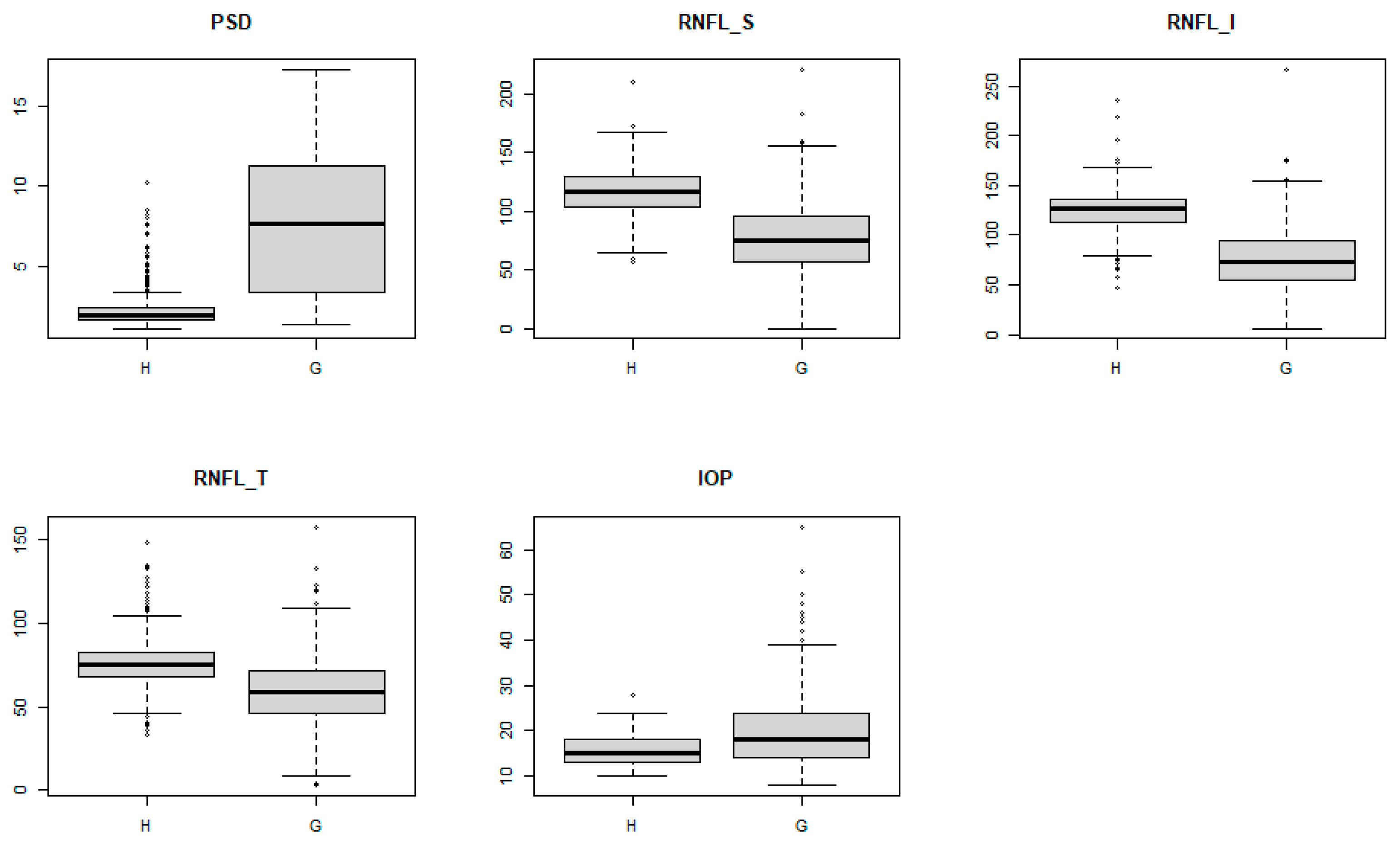
| No | Feature | Glaucoma Mean (SD 1) | Healthy Mean (SD) | p-Value |
|---|---|---|---|---|
| 1 | Sex | - | - | - |
| 2 | Age | 60.3 (14.13) | 51.7 (16.45) | <0.001 |
| 3 | GHT 2 | 4.28 (1.28) | 2.10 (1.53) | <0.001 |
| 4 | VFI 3 | 72.3 (32.24) | 95.7 (5.55) | <0.001 |
| 5 | MD 4 | −10.24 (9.72) | −2.33 (2.55) | <0.001 |
| 6 | Pattern standard deviation | 6.76 (4.27) | 2.49 (1.03) | <0.001 |
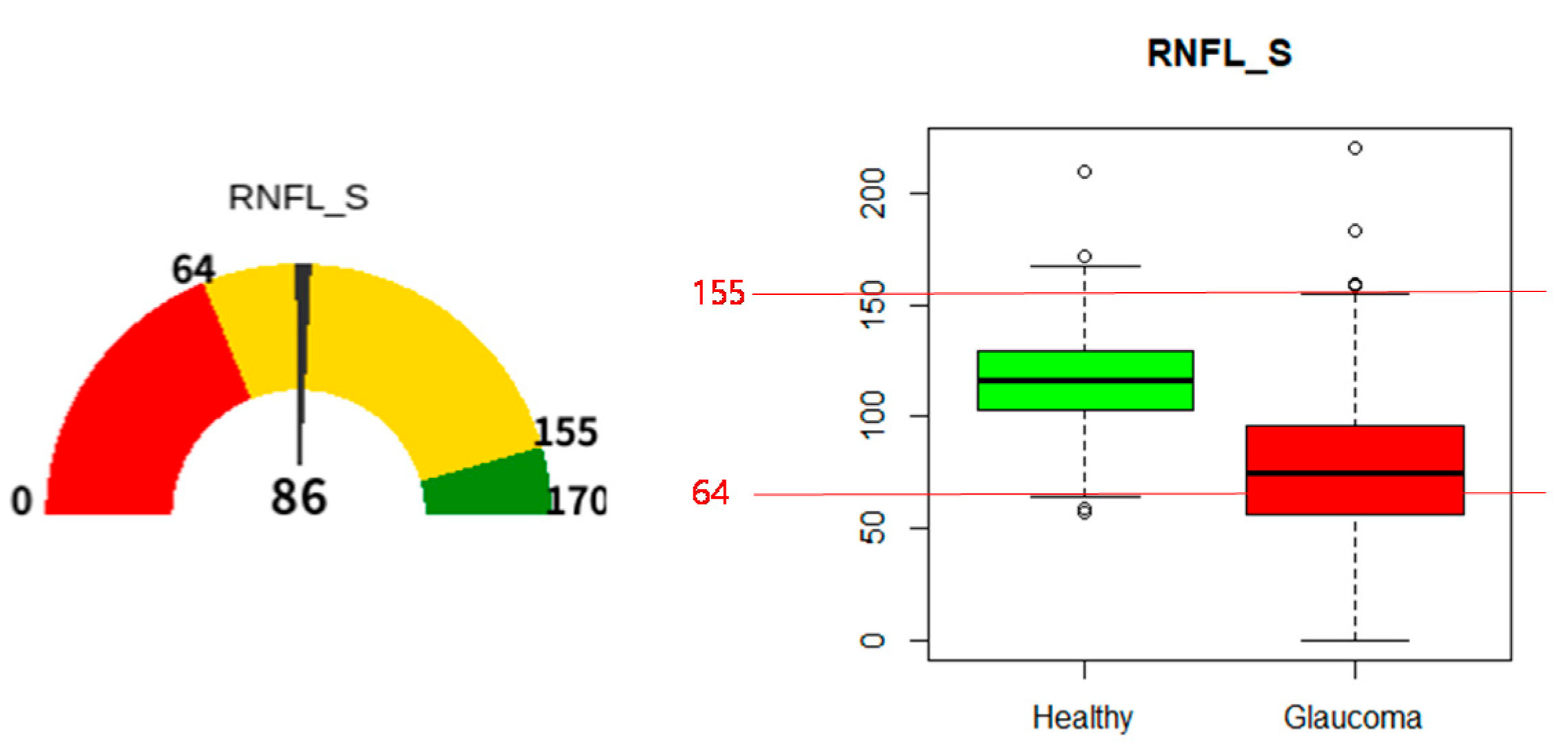
| 7 | RNFL 5 superior | 82.0 (27.71) | 112.6 (19.89) | <0.001 |
| 8 | RNFL Nasal | 56.1 (33.84) | 64.6 (16.64) | <0.001 |
| 9 | RNFL inferior | 79.9 (29.76) | 117.6 (20.28) | <0.001 |
| 10 | RNFL temporal | 58.6 (18.48) | 71.6 (15.01) | <0.001 |
| 11 | Mean of RNFL thickness | 68.5 (18.82) | 91.6 (12.60) | <0.001 |
| 12 | Intraocular pressure | 18.7 (8.69) | 15.7 (3.10) | <0.001 |
| 13 | Cornea thickness | 527.2 (34.15) | 530.1 (34.01) | <0.001 |
| 14 | BCVA 6 | 0.63 (0.31) | 0.73 (0.31) | 0.002 |
| 15 | Spherical equivalent | −1.63 (2.88) | −1.42 (3.08) | 0.12 |
| 16 | Axial length | 24.1 (1.81) | 24.1 (1.42) | 0.92 |
| 17 | Neuro-retinal rim | 0.79 (0.28) | 1.06 (0.21) | <0.001 |
| 18 | Cup | 0.47 (0.23) | 0.38 (0.43) | 0.16 |
| 19 | Disc | 1.97 (0.23) | 2.09 (0.43) | 0.25 |
| 20 | Mean of cup/disc ratio | 0.74 (0.11) | 0.65 (0.12) | <0.001 |
| 21 | vertical_cup/disc ratio | 0.73 (0.10) | 0.62 (0.16) | <0.001 |
| 22 | CNN 7 degree | 0.69 (0.18) | 0.53 (0.21) | <0.001 |
| No | Feature | Abbreviation | Source |
|---|---|---|---|
| 1 | pattern standard deviation | PSD | VF |
| 2 | RNFL superior | RNFL_S | RNFL optical coherence tomography (OCT) |
| 3 | RNFL inferior | RNFL_I | RNFL OCT |
| 4 | RNFL temporal | RNFL_T | RNFL OCT |
| 5 | intraocular pressure | IOP | IOP test |
| No | Hyper Parameter * | Value |
|---|---|---|
| 1 | booster | “gbtree” |
| 2 | eta | 0.7 |
| 3 | max_depth | 8 |
| 4 | gamma | 3 |
| 5 | subsample | 0.8 |
| 6 | colsample_bytree | 0.5 |
| 7 | objective | “multi:softprob” |
| 8 | eval_metric | “merror” |
| 9 | num_class | 2 |
| Metric | Support Vector Machine (SVM) | C50 | Random Forest (RF) | xgboost |
|---|---|---|---|---|
| Accuracy | 0.925 | 0.903 | 0.937 | 0.947 |
| Sensitivity | 0.933 | 0.874 | 0.924 | 0.941 |
| Specificity | 0.920 | 0.92 | 0.945 | 0.950 |
| AUC | 0.945 | 0.897 | 0.945 | 0.945 |
| Case | PSD | RNFL_S | RNFL_I | RNFL_T | IOP | Diagnosis | Prediction |
|---|---|---|---|---|---|---|---|
| 1 | 1.92 | 142 | 153 | 94 | 13 | Healthy | Healthy |
| 2 | 11.85 | 83 | 41 | 55 | 14 | Glaucoma | Glaucoma |
| 3 | 1.53 | 73 | 107 | 71 | 18 | Glaucoma | Healthy |
| 4 | 2.76 | 81 | 95 | 73 | 18 | Healthy | Glaucoma |
| 5 | 2.31 | 98 | 130 | 60 | 12 | Glaucoma | Healthy |
| Predict | |||
|---|---|---|---|
| Glaucoma | Healthy | ||
| Actual | Glaucoma | 916 | 59 |
| Healthy | 28 | 621 | |
| Case | PSD | RNFL_S | RNFL_I | RNFL_T | IOP |
|---|---|---|---|---|---|
| Correct prediction | 7.99 | 75.31 | 72.86 | 57.98 | 20.73 |
| Miss prediction | 2.65 | 111.12 | 122.69 | 71.25 | 15.78 |
| p-value | 2.23 × 10−55 | 2.74 × 10⁻²⁴ | 1.22 × 10⁻³⁴ | 3.09 × 10⁻¹⁰ | 1.39 × 10⁻¹⁷ |
| Case | PSD | RNFL_S | RNFL_I | RNFL_T | IOP |
|---|---|---|---|---|---|
| Correct prediction | 2.23 | 117.0 | 126.59 | 77.69 | 15.72 |
| Miss prediction | 3.84 | 90.40 | 91.21 | 61.89 | 15.68 |
| p-value | 1.64 × 10⁻³ | 1.74 × 10⁻⁸ | 2.66 × 10⁻¹¹ | 1.27 × 10⁻⁶ | 9.44 × 10⁻¹ |
Publisher’s Note: MDPI stays neutral with regard to jurisdictional claims in published maps and institutional affiliations. |
© 2021 by the authors. Licensee MDPI, Basel, Switzerland. This article is an open access article distributed under the terms and conditions of the Creative Commons Attribution (CC BY) license (http://creativecommons.org/licenses/by/4.0/).
Share and Cite
Oh, S.; Park, Y.; Cho, K.J.; Kim, S.J. Explainable Machine Learning Model for Glaucoma Diagnosis and Its Interpretation. Diagnostics 2021, 11, 510. https://doi.org/10.3390/diagnostics11030510
Oh S, Park Y, Cho KJ, Kim SJ. Explainable Machine Learning Model for Glaucoma Diagnosis and Its Interpretation. Diagnostics. 2021; 11(3):510. https://doi.org/10.3390/diagnostics11030510
Chicago/Turabian StyleOh, Sejong, Yuli Park, Kyong Jin Cho, and Seong Jae Kim. 2021. "Explainable Machine Learning Model for Glaucoma Diagnosis and Its Interpretation" Diagnostics 11, no. 3: 510. https://doi.org/10.3390/diagnostics11030510