Abstract
Volume of interest segmentation is an essential step in computer-aided detection and diagnosis (CAD) systems. Deep learning (DL)-based methods provide good performance for prostate segmentation, but little is known about the reproducibility of these methods. In this work, an in-house collected dataset from 244 patients was used to investigate the intra-patient reproducibility of 14 shape features for DL-based segmentation methods of the whole prostate gland (WP), peripheral zone (PZ), and the remaining prostate zones (non-PZ) on T2-weighted (T2W) magnetic resonance (MR) images compared to manual segmentations. The DL-based segmentation was performed using three different convolutional neural networks (CNNs): V-Net, nnU-Net-2D, and nnU-Net-3D. The two-way random, single score intra-class correlation coefficient (ICC) was used to measure the inter-scan reproducibility of each feature for each CNN and the manual segmentation. We found that the reproducibility of the investigated methods is comparable to manual for all CNNs (14/14 features), except for V-Net in PZ (7/14 features). The ICC score for segmentation volume was found to be 0.888, 0.607, 0.819, and 0.903 in PZ; 0.988, 0.967, 0.986, and 0.983 in non-PZ; 0.982, 0.975, 0.973, and 0.984 in WP for manual, V-Net, nnU-Net-2D, and nnU-Net-3D, respectively. The results of this work show the feasibility of embedding DL-based segmentation in CAD systems, based on multiple T2W MR scans of the prostate, which is an important step towards the clinical implementation.
1. Introduction
Prostate cancer is the most detected cancer in men and the second most common cause of cancer related death for men worldwide [1]. An early diagnosis of prostate cancer is essential for a better disease management [2]. Following reasonable suspicion of prostate cancer, based on elevated prostate-specific antigen (PSA) levels in blood and a digital rectal examination (DRE), the patient, in many countries, is likely to be referred to a pre-biopsy magnetic resonance imaging (MRI) to guide the collection of biopsies [3]. To improve the diagnostic process, the use of multi-parametric MRI (mpMRI) has been established through international guidelines [4,5,6]. Additionally, mpMRI has been employed in active surveillance programs to follow up the patients with indolent lesions [7], prostate cancer risk calculators [8], and treatment response monitoring [6,9]. Currently, the mpMR images are interpreted qualitatively by a radiologist, which is a tedious, time-consuming [10], and reader opinion-dependent [11,12] process. The resulting vulnerability to inter and intra-observer variability is problematic for clinical applications based on multiple scans in time, such as with active surveillance and response monitoring, where reproducibility of results is paramount. Automated computer-aided detection and diagnosis (CAD) systems have the potential to overcome the limitations of the traditional radiological reading by implementing quantitative models to automate, standardize, and support reproducible interpretations of radiological images [10,13,14,15].
Segmentation is an essential step for prostate CAD systems [13,15]. It helps locate the volume of interest (VOI), enabling subsequent extraction of quantitative features for radiomics-based approaches. Accurate segmentation is paramount as the following steps of a CAD system are dependent on it. Traditionally, the VOI segmentation is performed manually by a radiologist on T2-weighted (T2W) MR images. However, deep learning (DL)-based segmentation methods have shown promising performances [16,17,18,19,20]. Importantly, the inter-observer variability between DL-based segmentation methods and expert radiologists has been shown to be approximately equal to that between expert radiologists [21]. However, little is known about the reproducibility of DL-based segmentation methods for clinical MRI scans. To investigate the reproducibility of DL-based segmentation, radiomics shape features can be used. Shape features, like prostate volume, are already part of today’s clinical risk calculators for prostate cancer [8] and will likely play an important role in future radiomics-based clinical applications.
Recently, the reproducibility of several radiomics features, using manually segmented masks of the prostate on clinical MR images, has been investigated [22,23,24,25]. The study by Schwier et al. [22] was the only one that used segmentations of the whole prostate gland and zones. Their results showed high reproducibility of shape features, between manual segmentations on mpMRI scans, during a short time interval. Despite the useful information provided by these studies, they do not provide insight into the reproducibility of automatically generated segmentations. Furthermore, these studies did not focus on investigating the reproducibility of the segmentation masks themselves, as the manual segmentations were considered the reference. To the best of our knowledge, the reproducibility of DL-based segmentations of the prostate, on clinical MR images, has not been previously investigated.
The contribution of this study is the assessment of the reproducibility of DL-based segmentations of the whole prostate gland (WP), peripheral zone (PZ), and the remaining prostate zones (non-PZ; central, transition, and anterior fibro-muscular zones, combined) by comparing radiomics shape features from T2W MR images acquired with short time intervals.
2. Materials and Methods
2.1. Dataset
In this study, we used an in-house collected mpMRI dataset from 244 patients (median age = 65; range: 44–76 years) for retrospective analysis. This dataset came from a previous prospective study conducted by our group. The patients were examined at St. Olavs Hospital, Trondheim University Hospital, Trondheim, Norway between March 2015 and December 2017, due to suspicion of prostate cancer, via the Norwegian standardized care pathway, in which patients with elevated PSA and/or abnormal DRE results are referred for an initial mpMRI scan to identify suspicious cancerous tissue [26]. If the radiologist detected suspicious tissue in the aforementioned prospective study, patients were randomly selected for either standard transrectal ultrasound-guided biopsy or in-bore targeted MR-guided biopsy. The latter group (n = 62), therefore, had two mpMRI scans. The Regional Committee for Medical and Health Research Ethics (REC Central Norway) approved the use of the dataset (identifiers 2013/1869 and 2017/576). All the patients signed informed consent prior to the initiation of the prospective study.
The dataset (T2W images) was split into a training set (n = 182), to train the DL-based segmentation networks, and an investigation set (n = 62), to investigate the reproducibility of shape features extracted from the segmented prostate masks. The investigation set was acquired at two different time points: first, at the initial visit for the detection of prostate cancer (scan 1) and second, during an MR-guided biopsy procedure (scan 2). The interval between scans ranged from 1–71 (median = 7) days. Patients in the collected dataset with two scans were assigned to the investigation set. Those who had only one scan, acquired at the initial visit for detection of prostate cancer, were assigned to the training set.
T2W MRI was performed on a Magnetom Skyra 3 T MRI system (Siemens Healthineers, Erlangen, Germany) with a turbo spin-echo sequence. The scanning parameters details are given in Table 1.

Table 1.
Summary of MRI scanning parameters.
2.2. Prostate Segmentation
Manual segmentation of PZ and non-PZ for the in-house collected dataset was performed using ITK-SNAP [27] (version 3.6.0) by a radiology resident (E.S.) at St. Olavs Hospital, Trondheim University Hospital, Trondheim, Norway, under the supervision of a radiologist (S.L.) with more than 10 years’ experience in prostate imaging. PZ and non-PZ masks were used to generate the WP masks by merging. Lesion segmentation was beyond the scope of this study and was, therefore, not considered.
The DL-based segmentation was performed using three different convolutional neural networks (CNNs), which are all variants of the famous U-Net with an encoder-decoder scheme, along with long skip connections [28], further referred to as V-Net [18], nnU-Net-2D [16], and nnU-Net-3D [16]. These three networks were chosen for their popularity, good performance, and public availability. Unlike U-Net, V-Net is a residual learning network that replaces the maximum pooling operation with strided convolutions and the ReLU activation functions with PReLU activation functions [18]. On the other hand, nnU-Net does not introduce a new architecture, but it uses a 2D or 3D U-Net network with automatic self-configuration of pre-processing, network architecture, training, and post-processing [16]. nnU-Net-2D performed the segmentation on a 2D slice-by-slice basis, whereas V-Net and nnU-Net-3D performed the segmentation on a 3D volume basis. Prior to segmentation, all images were pre-processed in accordance with the corresponding segmentation method. The segmentation pre-processing, training, and testing were performed on a single NVIDIA Tesla P100 PCIe 16 GB GPU in Ubuntu 18.04.4 LTS.
V-Net was implemented with PyTorch [29] (version 1.4.0) using Python (version 3.6.9; Python Software Foundation, Wilmington, DE, USA) to generate two separate models for WP and PZ, which were used to generate non-PZ masks by subtraction. Each of the V-Net models was trained for 16,000 iterations with a batch size of 2. Adaptive moment estimation with momentum of 0.99, a weight decay of 1 × 10⁻⁸, and an initial learning rate of 1 × 10⁻⁴ were used for learning the network weights. The training time for each of the models was 10 h with cuDNN acceleration.
nnU-Net-2D (version 2.1) and nnU-Net-3D (version 2.1) were implemented with PyTorch (version 1.7.0) using Python (version 3.6.10) to generate one model for both PZ and non-PZ, which were used to generate the WP masks by merging. The nnU-Net-2D model was trained for 978 epochs with a batch size of 22. Stochastic gradient descent with Nesterov Momentum of 0.99, a weight decay of 3 × 10⁻⁵, and an initial learning rate of 1 × 10⁻² were used for learning the network weights. The training time of the model was 55 h with cuDNN acceleration. The nnU-Net-3D model was trained for 625 epochs with a batch size of 2. Stochastic gradient descent with Nesterov Momentum of 0.99, a weight decay of 3 × 10⁻⁵, and an initial learning rate of 1 × 10⁻² were used for learning the network weights. The training time of the model was 88 h with cuDNN acceleration.
The DL-based segmentations were post-processed to only keep the largest 3D connected component, using a pixel connectivity of 26.
2.3. Feature Extraction
Shape features were extracted from the 3D segmentation masks (Manual or DL-based) of PZ, non-PZ, and WP using Pyradiomics [30] (version 3.0; an open-source Python package). The following 14 shape features were extracted: Elongation, Flatness, Least Axis Length, Major Axis Length, Maximum 2D diameter (Column), Maximum 2D diameter (Row), Maximum 2D diameter (Slice), Maximum 3D diameter, Mesh Volume, Minor Axis Length, Sphericity, Surface Area, Surface Area to Volume ratio, and Voxel Volume. A detailed description of the features can be found at [31].
2.4. Investigation of Reproducibility
Reproducibility is defined as the “variability in measurements made on the same subject, but under changing conditions” [32]. The variability and reproducibility are inversely related, i.e., the higher the variability, the lower the reproducibility. In this work, scan 1 and scan 2 were performed on the same patients, but at different time points and using different scanning procedures.
To investigate the reproducibility, all extracted features from the two scans of 62 patients’ scans, using the manual and post-processed DL-based segmentations, were included. The reproducibility for each of the 14 shape features was investigated, separately, for each of the CNNs and compared to that of the corresponding feature from the manual segmentations. Furthermore, the DL-based segmentation performance and segmentation volume (Voxel Volume feature) in scan 1 and scan 2 were compared to those of manual segmentations.
In addition, the reproducibility results were compared to the corresponding results where (1) the post-processing step was excluded, and (2) patients with a poor segmentation quality score were excluded. To enable the last comparison, our previously proposed automated segmentation quality control system (SQCS) [33] was implemented, and the patients with a quality score of less than 85 for scan 1 or/and scan 2 were excluded from further analysis. As per [33], the SQCS was implemented using pre-processed T2W images and WP segmentations.
2.5. Statistical Analysis
The dice similarity coefficient (DSC) [34], between manual and DL-based segmentations, was calculated as a metric of segmentation performance.
The two-way random, single score intra-class correlation coefficient (ICC) [35,36] was used to measure the inter-scan reproducibility of each feature for each CNN and the manual segmentations. Statistical significance between features, from manual segmentation and each CNN, and between features, from including and excluding the post-processing step, was based on overlapping 95% confidence intervals (CI) [37].
The paired Wilcoxon signed rank test [38], followed by Benjamini–Hochberg correction for multiple testing [39], was used to assess the differences in DSC, the ICC values between VOIs, and segmentation volume between networks and scans.
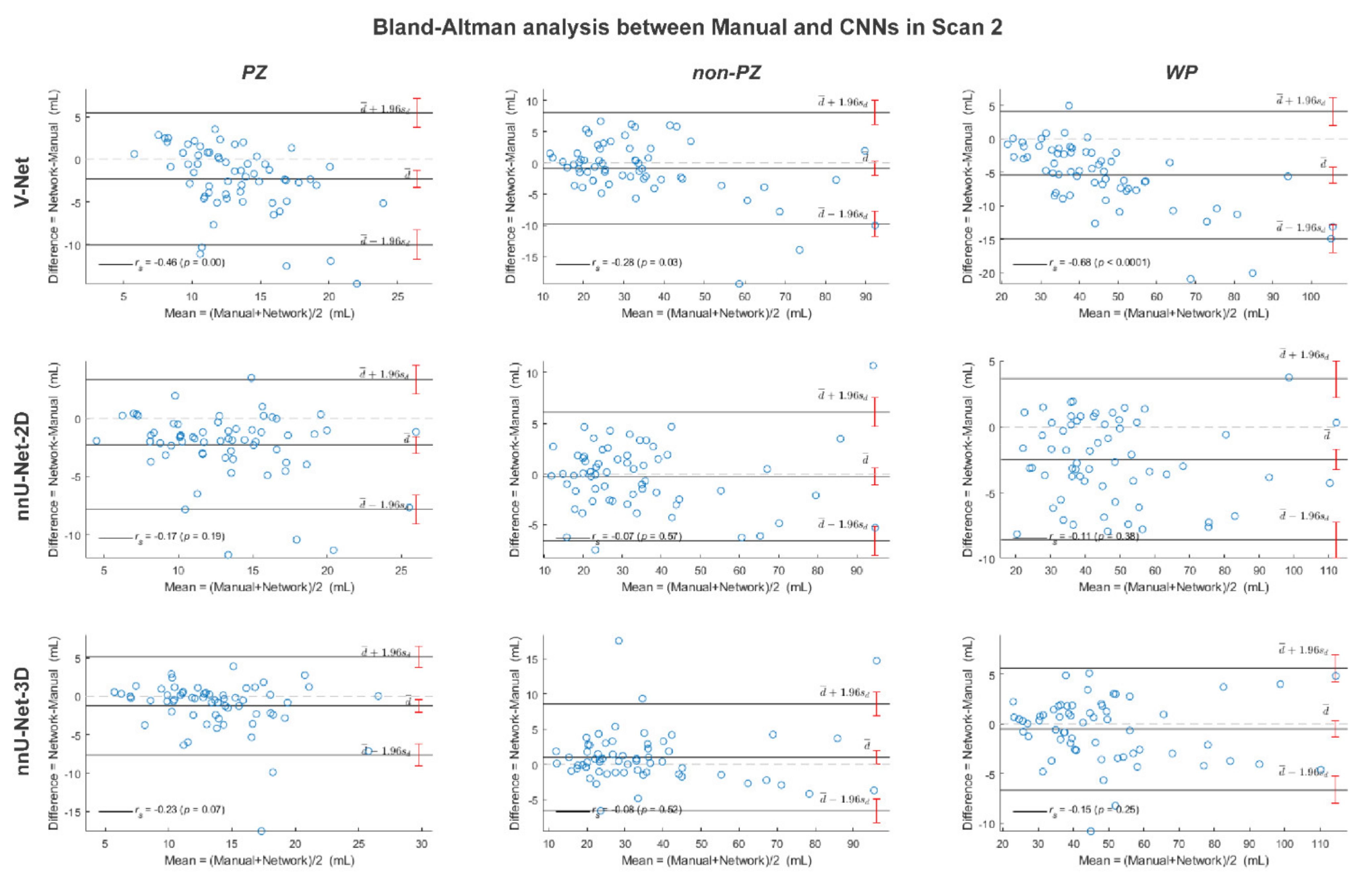
The Bland–Altman analysis [40] and Spearman’s rank test [38] were performed to assess the correlation between the segmentation volumes for scan 1 and scan 2 and between the segmentation volumes of each of the CNNs and the manual segmentations in scan 1 and scan 2.
To assess the difference in feature reproducibility, before and after implementing the SQCS, a permutation test [38] with 1000 runs was performed for each CNN. In each of these 1000 runs, the ICC value was calculated after randomly excluding the same number of cases as excluded by the SQCS. The improvement in ICC, after applying the SQCS, was considered significant if less than 50/1000 randomly permuted values were higher or equal to the ICC after the SQCS implementation.
MATLAB R2019b (MathWorks, Natick, MA, USA) was used for statistical analysis.
3. Results
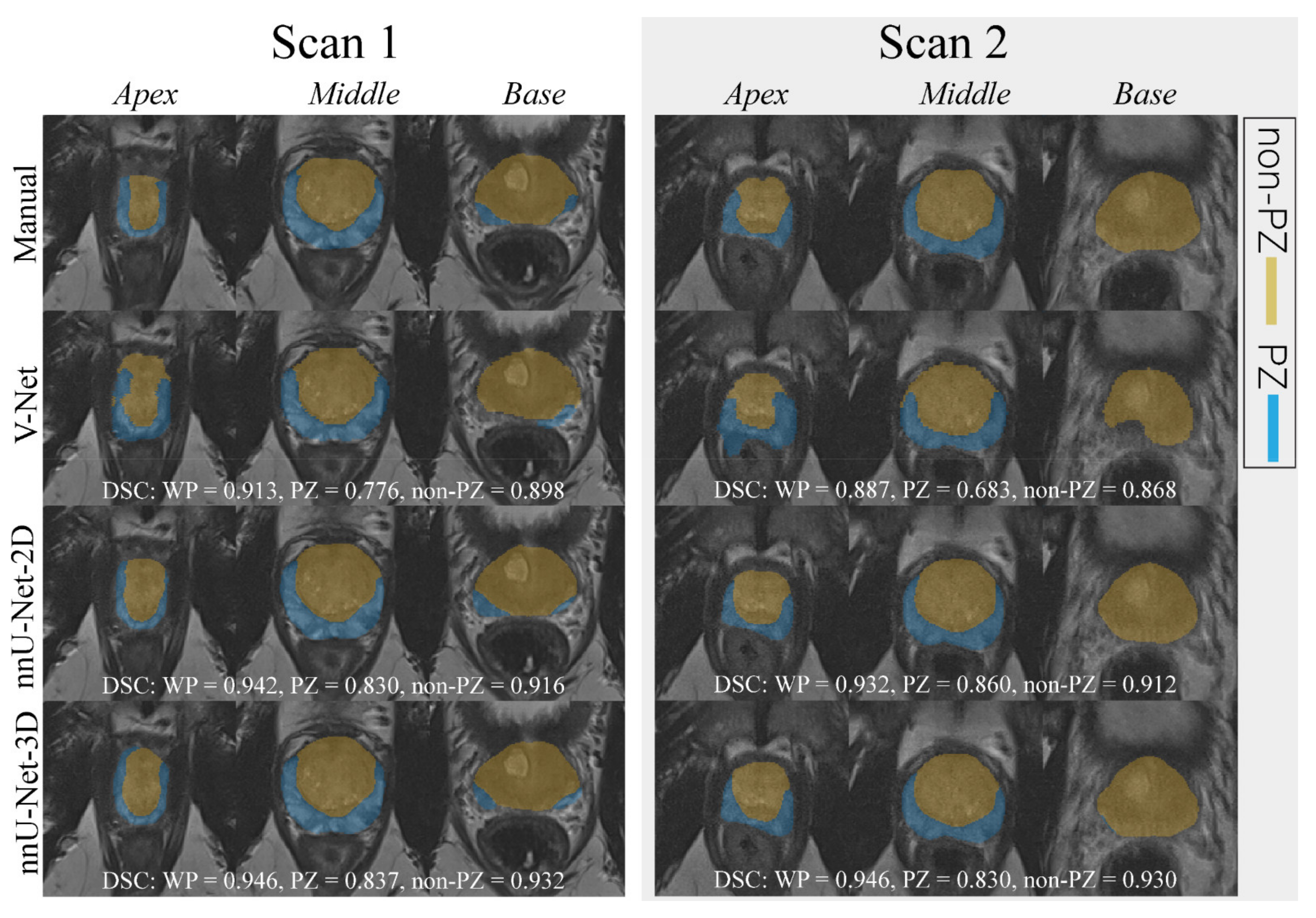
An example case segmented with the three investigated CNNs is shown in Figure 1.
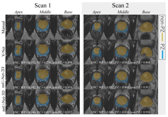
Figure 1.
The middle slice for the whole prostate, apex, and base of a randomly selected case was segmented (peripheral zone (PZ) and the remaining prostate zones (non-PZ)) by different approaches for scan 1 and 2. For each network, the dice similarity coefficient (DSC) of the 3D segmented volume is reported for the whole prostate gland (WP), PZ, and non-PZ.
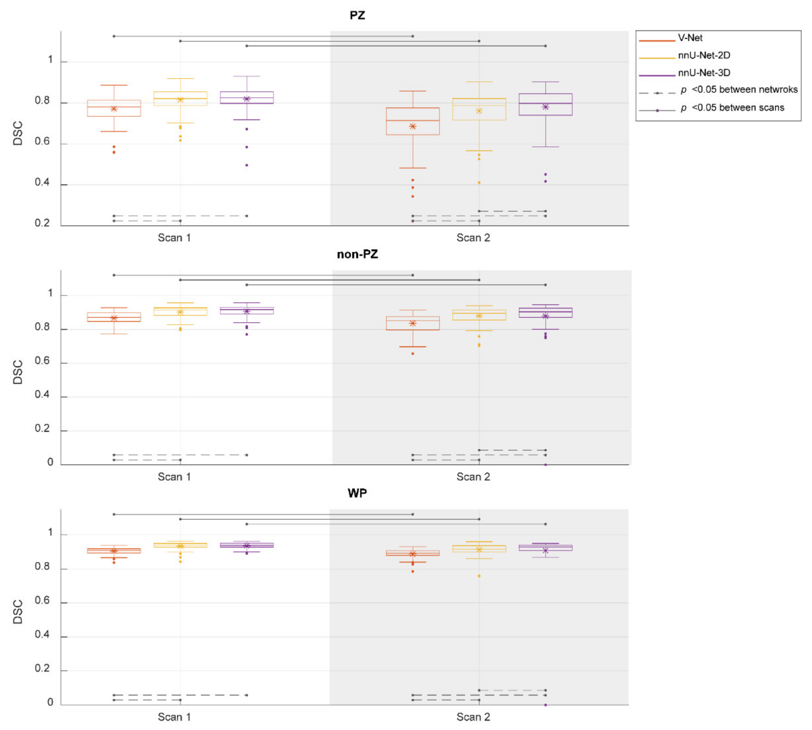
Figure 2 shows the performance of the investigated CNNs segmentations. The median DSCs were 0.781, 0.821, and 0.825 in PZ; 0.871, 0.916, and 0.917 in non-PZ; 0.909, 0.937, and 0.940 in WP for V-Net, nnU-Net-2D, and nnU-Net-3D, respectively, in scan 1; 0.714, 0.788, and 0.798 in PZ; 0.853, 0.896 and 0.904 in non-PZ; 0.893, 0.917, and 0.929 in WP for V-Net, nnU-Net-2D, and nnU-Net-3D, respectively, in scan 2. Median of DSC difference between the scans (scan 2–scan 1) was −9.49%, −4.06% and −3.65% in PZ; −3.12%, −1.80% and −1.08% in non-PZ; −1.98%, −1.95% and −1.39% in WP for V-Net, nnU-Net-2D and nnU-Net-3D, respectively. V-Net performed significantly lower (p < 0.001) than nnU-Net-2D and nnU-Net-3D in both of the scans and all of VOIs. nnU-Net-3D performed significantly higher (p < 0.01) than nnU-Net-2D in scan 2 for all of VOIs. In addition, each of the CNNs performed significantly lower (p < 0.001) in scan 2 compared to scan 1.
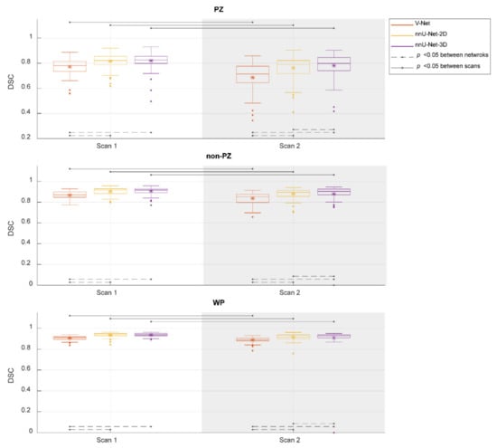
Figure 2.
The performance (dice similarity coefficient-DSC) of the segmentation methods for the whole prostate gland (WP), peripheral zone (PZ), and the remaining prostate zones (non-PZ). The Manual segmentations were considered as reference. The means are denoted by  , while the outliers are denoted by ●.
 , while the outliers are denoted by ●.
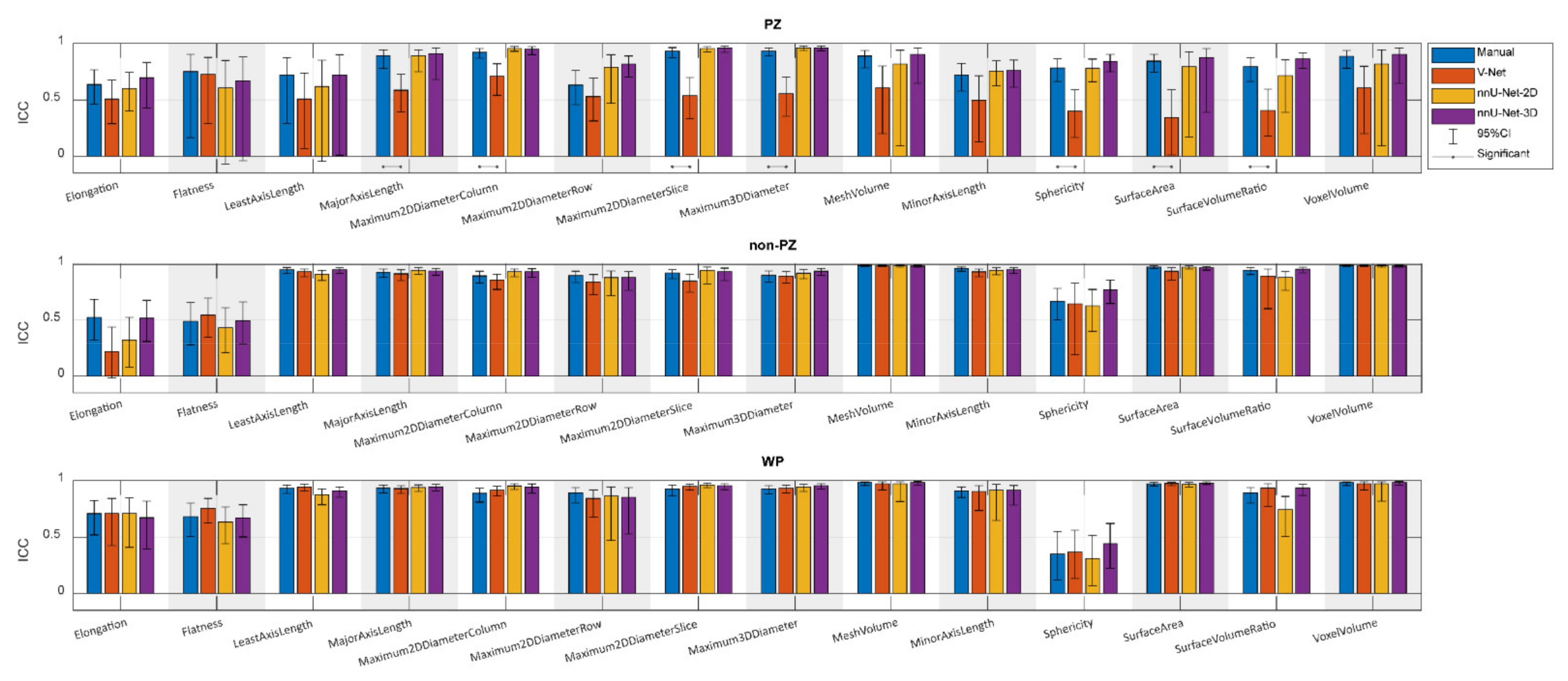
Figure 3 shows the ICCs from the extracted shape features from scan 1 and scan 2, where the segmentation post-processing step was included, and the segmentation quality control system was not implemented, demonstrating that the reproducibility of DL-based segmentation is comparable to manual segmentation for all networks (14/14 features), except for V-Net in PZ (7/14 features). In both manual and DL-based segmentations, Elongation, Flatness, and Sphericity had a remarkably lower ICC than the other features in WP and non-PZ. nnU-Net-3D showed higher reproducibility than the rest of the CNNs with a median difference in ICC equal to 54.03% and 9.06% in PZ; 3.95% and 0.38% in non-PZ; 0.95% and 1.09% in WP with V-Net and nnU-Net-2D, respectively. Additionally, in most cases, feature reproducibility in the non-PZ and WP was higher than in the PZ. V-Net had significantly higher (p < 0.01) ICCs in non-PZ and WP compared to PZ.
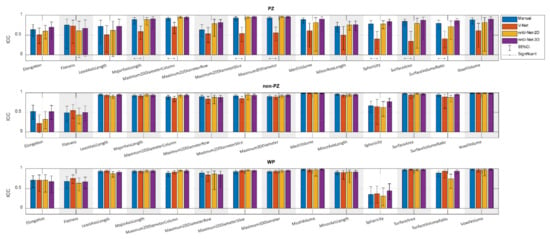
Figure 3.
The single score intra-class correlation coefficient (ICC), with the 95% confidence interval (95% CI), of the shape features extracted from the whole prostate gland (WP), peripheral zone (PZ), and the remaining prostate zones (non-PZ) for the investigated methods, where the segmentation post-processing step was included, and the segmentation quality control system was not implemented.
Comparing reproducibility when including (Figure 3) and excluding (Figure A1) the segmentation post-processing step, while SQCS was not implemented in any of them, shows that the reproducibility is remarkably enhanced when including the segmentation post-processing step. The ICC, after including the segmentation post-processing step, was significantly better in (4/14) features for V-Net in non-PZ; (14/14), (12/14), and (13/14) features for nnU-Net-2D in PZ, non-PZ, and WP, respectively; (13/14), (14/14), and (13/14) features for nnU-Net-3D in PZ, non-PZ, and WP, respectively.
Similarly, the reproducibility was increased with the SQCS implementation (Figure A2) compared to no implementation (Figure 3); the segmentation post-processing step was included in both cases. After implementing the SQCS, 10, 11, and 6 patient’s segmentations were excluded from V-Net, nnU-Net-2D, and nnU-Net-3D, respectively. The ICC after implementing the SQCS was significantly better in (3/14), (2/14), and (3/14) features for V-Net in PZ, non-PZ, and WP, respectively; in (7/14) and (2/14), features for nnU-Net-2D in non-PZ, and WP, respectively; in (1/14) and (5/14) features for nnU-Net-3D in non-PZ and WP, respectively.
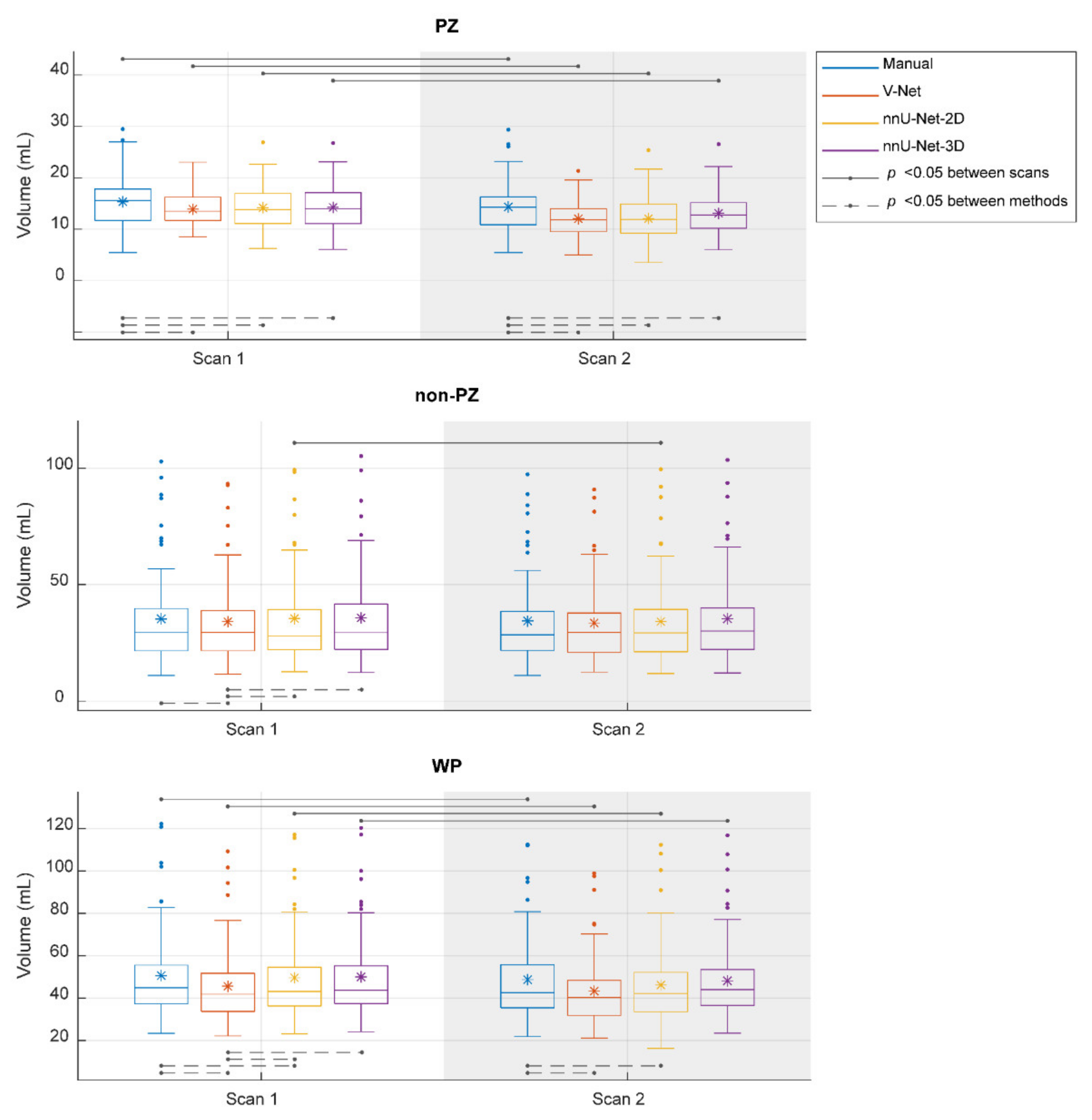
The segmented volume (Voxel Volume feature) was further investigated, as it is an important and in-use biomarker for multiple clinical applications [41,42,43]. Its ICC score, when the segmentation post-processing step was included and the SQCS was not implemented, was 0.888, 0.607, 0.819, and 0.903 in PZ; 0.988, 0.967, 0.986, and 0.983 in non-PZ; 0.982, 0.975, 0.973, and 0.984 in WP for manual, V-Net, nnU-Net-2D, and nnU-Net-3D, respectively. Figure 4 shows that the segmented volume was significantly lower in scan 2, compared to scan 1, for all the methods in PZ and WP (p < 0.001) and for nnU-Net-2D in non-PZ (p = 0.003). Bland–Altman analysis shows a similar bias for manual and DL-based methods (Figure A3). Median of volume difference between the scans (scan 2–scan 1) was −4.33%, −3.58%, −5.80%, and −3.32% in WP for manual, V-Net, nnU-Net-2D, and nnU-Net-3D, respectively. It also shows a small bias between the volumes of the DL-based and manual segmentations in scan 1 (Figure A4) and scan 2 (Figure A5). It was noticed that PZ has higher bias between scans and methods than non-PZ and WP. V-Net has also showed a slightly higher bias between scans and methods than nnU-Net-2D and nnU-Net-3D.
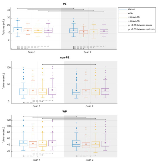
Figure 4.
The segmented volume of the whole prostate gland (WP), peripheral zone (PZ), and the remaining prostate zones (non-PZ) from the investigated methods in scan 1 and scan 2. The means are denoted by  , while the outliers are denoted by ●.
 , while the outliers are denoted by ●.
4. Discussion
VOI segmentation is an essential step in CAD systems. DL-based methods provide good performance for prostate segmentation, but little is known about their reproducibility. The reproducibility of radiomics shape features can be used as an indicator of the segmentation reproducibility. Therefore, in this paper, we investigated the reproducibility of the shape features extracted from DL-based segmentations of the WP, PZ, and non-PZ on T2W MR images, acquired with short time intervals (median = 7 days), and compared them to those of manual segmentations. Prostate gland volume is proportionally related to benign enlargement [44] and inversely related to prostate cancer [45]. Both of those conditions usually require long time to develop, thus no significant change in prostate gland volume is expected during a short time interval. Shape features, such as prostate volume, used to measure the PSA-density (PSA level/prostate volume) [46], are already part of today’s clinical risk calculators for prostate cancer [8] and will likely play an important role in future radiomics-based clinical applications. For clinical applications based on multiple scans in time, like active surveillance, it is key that extracted features are both accurate and reproducible.
The DSC values were in line with those expected from the literature [16,18], indicating that the trained networks have state-of-the-art performance. nnU-Net-3D had the best overall segmentation accuracy, while V-Net showed the lowest segmentation accuracy comparable to the manual segmentations. This work extends previous studies, showing the excellent performance of nnU-Net, specifically the 3D volume basis model, on a wide variety of medical image segmentation tasks [16]. The DSC values were slightly lower in scan 2 compared to scan 1. This is probably due to the nature of the segmentation training set, which consisted of cases acquired with a scan protocol similar to that of scan 1.
Based on ICCs of the shape features, nnU-Net-2D and nnU-Net-3D were shown to have comparable reproducibility to manual segmentations in all VOIs. WP and non-PZ showed higher ICCs compared to PZ, which was expected due to the low PZ segmentation performance. nnU-Net-3D provided higher ICCs compared to the other CNNs, which was expected as it had the highest segmentation performance among CNNs. Overall, the results show that DL-based segmentation methods can generate highly intra-patient reproducible masks for T2W images of the prostate. Good reproducibility gives potential for picking up changes in the prostate when they appear, an important step towards the clinical implementation of prostate CAD systems, based on multiple T2W MRI scans.
Including a post-processing step to the segmentation, where only the largest connected component in 3D volume is kept, was shown to remarkably enhance the features reproducibility. Similarly, the implementation of the SQCS significantly increased the reproducibility. Therefore, the implementation of these two post-processing steps in a CAD system pipeline is recommended to assure highly reproducible shape features. In clinical applications, the cases with low segmentation quality score, predicted by the SQCS, should be either referred to a radiologist for manual intervention or re-segmented using another CNN.
One possible explanation for the lower ICC of Elongation, Flatness, and Sphericity in WP and non-PZ is that the prostate gland in scan 2 was potentially compressed due to a guiding probe for the biopsy needle inside the patient’s rectum during the image acquisition. Moreover, the patients were scanned in prone position during scan 2, in contrast to scan 1, where they were scanned in supine position. The probe and the prone position would, indeed, not alter the volume of the prostate but might deform its shape slightly. In their study, Osman et al. [47] have investigated the endorectal coil effect on the WP volume and shape during prostate T2W MRI and concluded that, despite shape deformation, there is no significant change in the WP volume between including and excluding the endorectal coil. Although the needle guiding probe differs from the endorectal coil, its impact may be expected to be similar. In addition, the prostate gland might deform between scans due to other factors, e.g., different bladder/bowel loading, which were not taken into account in this study. The shape deformation may have had an impact on the decision of including or excluding a slice from the segmentation. We noticed that, overall, scan 2 had a lower number of segmented slices than scan 1. Median of the segmented slices number was 14, 14, 14, and 14 in WP for manual, V-Net, nnU-Net-2D, and nnU-Net-3D, respectively, in scan 1 and 13, 13.5, 13, and 14 in WP for manual, V-Net, nnU-Net-2D, and nnU-Net-3D, respectively, in scan 2. Although the difference between the numbers is small (≈1 slice), it will influence the segmented volumes, which were indeed slightly lower in scan 2 than in scan 1.
The reproducibility of the segmented volume might be the most important among the 14 investigated features. WP volume is used by the radiologist to measure the PSA-density, which is part of today’s clinical risk calculators [8], and can be used as a biomarker to evaluate prostate cancer progression and the need for re-biopsy [43]. An alternative biomarker to the traditional PSA-density is the zonal adjusted PSA-density, which depends on the segmented volume from various prostate gland zones, i.e., non-PZ volume [48,49]. Our study shows that the segmented volume feature is highly reproducible, and in agreement with manual volumes on both zonal and whole prostate-level.
In their work, Schwier et al. [22] used manual segmentations to assess the reproducibility of radiomics features on prostate T2W MR images. Their focus was mainly on the reproducibility of the radiomics textural features under different settings, but they have also included results on some of the shape features reproducibility. Although there is some similarity between their work and ours, our work focused on the reproducibility of DL-based segmentations. Like in our work, Schwier et al. showed that the reproducibility of shape features is high. Furthermore, they showed that the segmented volume reproducibility is higher in WP than in PZ, which was also in line with our findings. The high ICC values found in this work suggest that all the shape features, except for Elongation, Flatness, and Sphericity, extracted using DL-based segmentation methods, can be used in clinical applications based on multiple scans without being concerned about their reproducibility.
In this work, we used a dataset from prostate cancer patients referred and scanned according to prevailing guidelines. Consequently, the results represent the reproducibility of the DL-based segmentations in a real clinical setting. Nevertheless, our study has some limitations. The patient cohort was relatively small, and it was obtained from a single center. Conducting a multicenter study in the future might give additional insight on the reproducibility of DL-based segmentation across institutions. Moreover, the manual segmentations in this study have been performed by one reader. A set of manual segmentations, where multiple readers are included, will facilitate additional comparisons, which might provide us with more information, but this can be considered for a future work.
5. Conclusions
We investigated the reproducibility of the shape features, extracted from DL-based segmentations, of the prostate gland and zones on T2W MR images acquired with short time intervals. The reproducibility of the best-performing DL-based prostate segmentation methods is comparable to that of manual segmentations, which is important for clinical applications, based on multiple scans in time.
Author Contributions
Conceptualization, M.R.S.S., T.F.B. and M.E.; methodology, M.R.S.S., T.F.B. and M.E.; formal analysis, M.R.S.S.; investigation, M.R.S.S., K.M.S., E.S., H.B., T.F.B. and M.E.; resources, K.M.S., E.S., S.L. and H.B.; data curation, M.R.S.S., K.M.S., E.S. and S.L.; writing—original draft preparation, M.R.S.S.; writing—review and editing, M.R.S.S., K.M.S., E.S., S.L., H.B., T.F.B. and M.E.; supervision, T.F.B. and M.E. All authors have read and agreed to the published version of the manuscript.
Funding
This research was funded by the Norwegian University of Science and Technology (NTNU) Biotechnology (grant number 81770928), the Research Council of Norway (grant number 295013) and the liaison committee between the Central Norway Regional Health Authority and Central Norway Regional Health Authority (grant number 17/38297).
Institutional Review Board Statement
The study was conducted according to the guidelines of the Declaration of Helsinki, and the dataset use was approved by the Regional Committee for Medical and Health Research Ethics (REC Central Norway; identifiers 2013/1869 and 2017/576; approval dates: 27 March 2014 and 05 May 2017, respectively).
Informed Consent Statement
Written informed consent, including consent for publication, was obtained from the patient.
Data Availability Statement
The dataset used in this study are not publicly available due to specific institutional requirements governing privacy protection.
Acknowledgments
We would like to thank Fausto Milletari from the Technical University of Munich (Munich, Germany) and Fabian Isensee from the German Cancer Research Center (Heidelberg, Germany) for making their segmentation methods publicly available.
Conflicts of Interest
The authors declare no conflict of interest. The funders had no role in the design of the study; in the collection, analyses, or interpretation of data; in the writing of the manuscript, or in the decision to publish the results.
Appendix A
Figure A1.
The single score intra-class correlation coefficient (ICC) with its 95% confidence interval (95%CI) of the shape features extracted from the whole prostate gland (WP), peripheral zone (PZ) and the remaining prostate zones (non-PZ) for the investigated methods, where the segmentation post-processing step was skipped and the segmentation quality control system was not implemented.
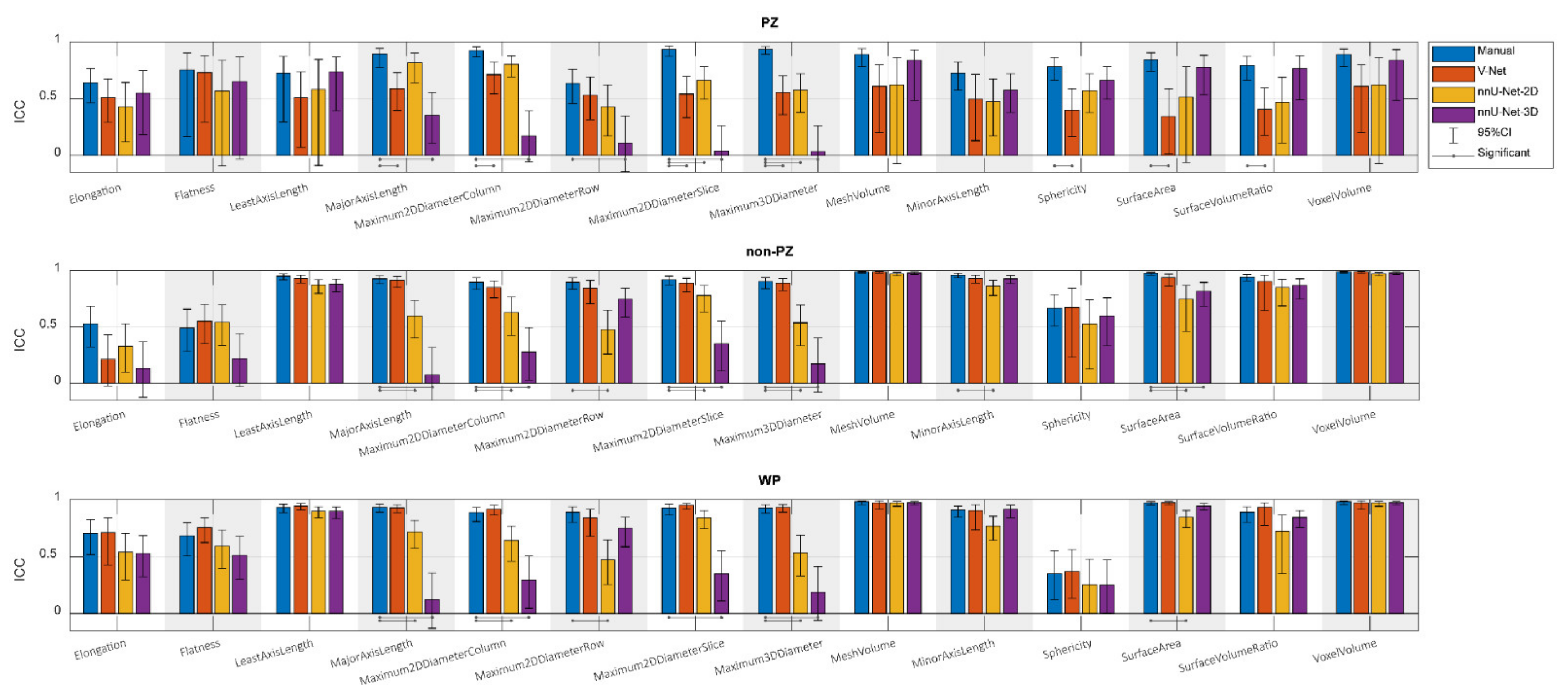
Figure A2.
The single score intra-class correlation coefficient (ICC) with its 95% confidence interval (95%CI) of the shape features extracted from the whole prostate gland (WP), peripheral zone (PZ) and the remaining prostate zones (non-PZ) for the investigated methods, where the segmentation post-processing step was included and the segmentation quality control system was implemented. The patients with a quality score less than 85 for scan 1 or/and scan 2 were excluded.
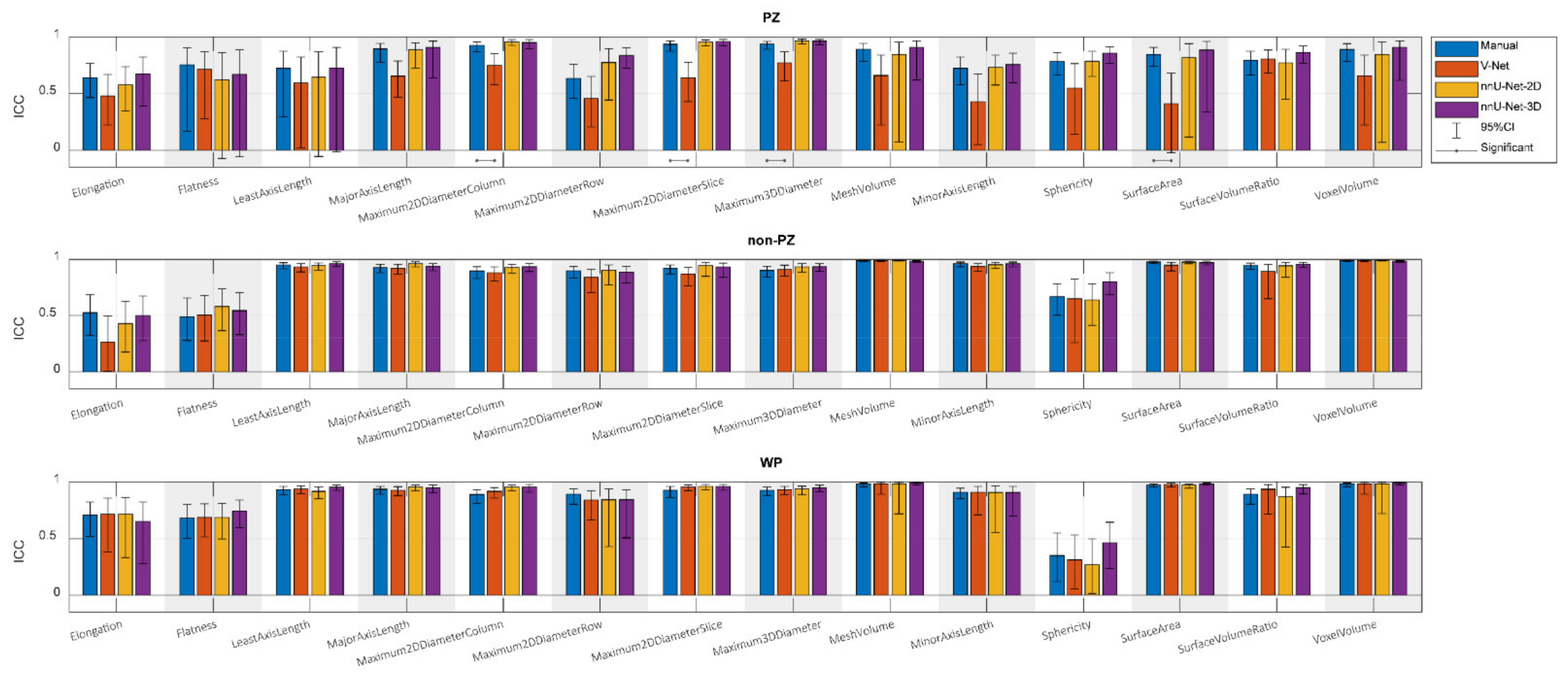
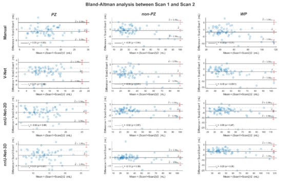
Figure A3.
The Bland-Altman plots for the agreement between scan 1 and scan 2 volumes from the whole prostate gland (WP), peripheral zone (PZ) and the remaining prostate zones (non-PZ) for the investigated methods. The 95% confidence interval limits for mean and agreement limits are denoted by Ι, while the cases are denoted by ○.
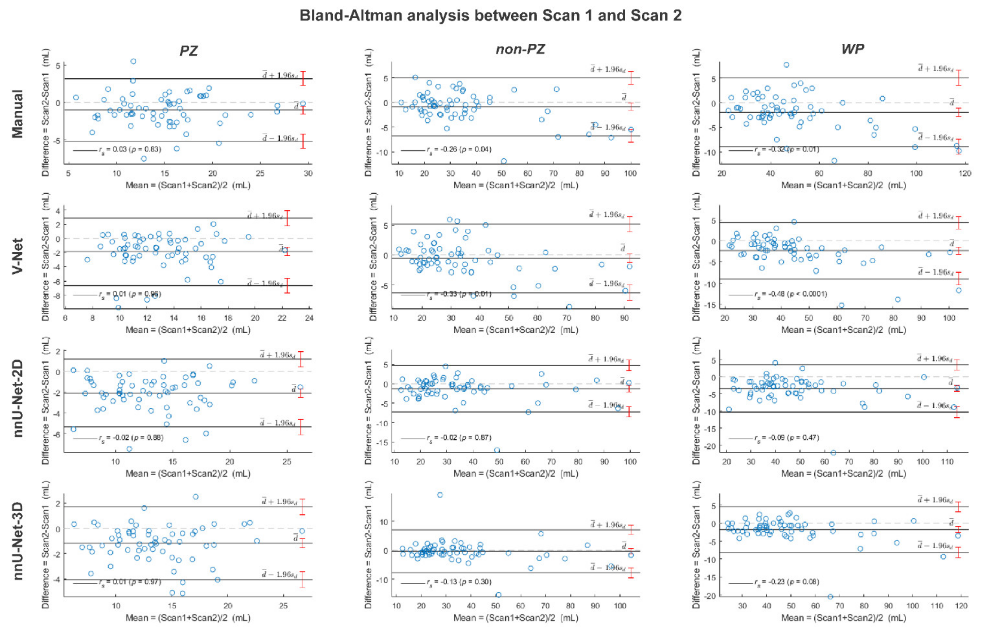
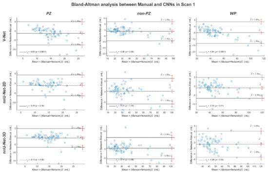
Figure A4.
The Bland-Altman plots for the agreement between manual and rest of the investigated methods volumes from the whole prostate gland (WP), peripheral zone (PZ) and the remaining prostate zones (non-PZ) in scan 1. The 95% confidence interval limits for mean and agreement limits are denoted by Ι, while the cases are denoted by ○.
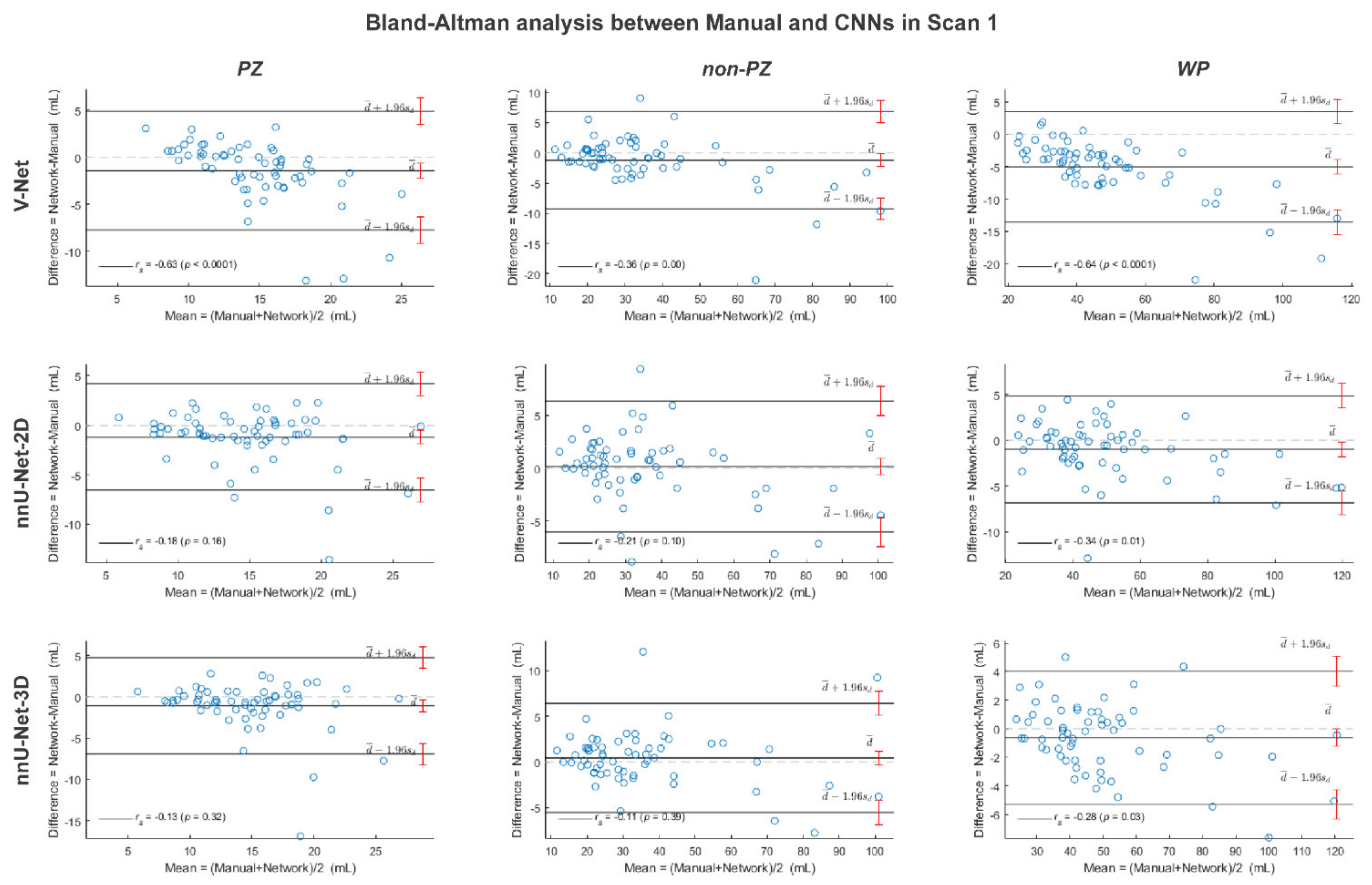
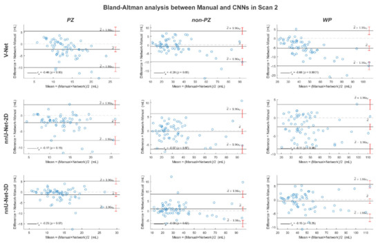
Figure A5.
The Bland-Altman plots for the agreement between manual and rest of the investigated methods volumes from the whole prostate gland (WP), peripheral zone (PZ) and the remaining prostate zones (non-PZ) in scan 2. The 95% confidence interval limits for mean and agreement limits are denoted by Ι, while the cases are denoted by ○.
References
- Bray, F.; Ferlay, J.; Soerjomataram, I.; Siegel, R.L.; Torre, L.A.; Jemal, A. Global cancer statistics 2018: GLOBOCAN estimates of incidence and mortality worldwide for 36 cancers in 185 countries. CA A Cancer J. Clin. 2018, 68, 394–424. [Google Scholar] [CrossRef] [Green Version]
- Mottet, N.; Bellmunt, J.; Bolla, M.; Briers, E.; Cumberbatch, M.G.; de Santis, M.; Fossati, N.; Gross, T.; Henry, A.M.; Joniau, S.; et al. EAU-ESTRO-SIOG guidelines on prostate cancer. Part 1: Screening, diagnosis, and local treatment with curative intent. Eur. Urol. 2017, 71, 618–629. [Google Scholar] [CrossRef]
- Ahdoot, M.; Wilbur, A.R.; Reese, S.E.; Lebastchi, A.H.; Mehralivand, S.; Gomella, P.; Bloom, J.; Gurram, S.; Siddiqui, M.; Pinsky, P.; et al. MRI-targeted, systematic, and combined biopsy for prostate cancer diagnosis. N. Engl. J. Med. 2020, 382, 917–928. [Google Scholar] [CrossRef] [PubMed]
- Barentsz, J.O.; Richenberg, J.; Clements, R.; Choyke, P.; Verma, S.; Villeirs, G.; Rouviere, O.; Løgager, V.B.; Fütterer, J.J. ESUR prostate MR guidelines 2012. Eur. Radiol. 2012, 22, 746–757. [Google Scholar] [CrossRef] [PubMed] [Green Version]
- Turkbey, B.; Rosenkrantz, A.B.; Haider, M.A.; Padhani, A.; Villeirs, G.; Macura, K.J.; Weinreb, J.C. Prostate imaging reporting and data system version 2.1: 2019 update of prostate imaging reporting and data system version 2. Eur. Urol. 2019, 76, 340–351. [Google Scholar] [CrossRef]
- Weinreb, J.C.; Barentsz, J.O.; Choyke, P.L.; Cornud, F.; Haider, M.A.; Macura, K.J.; Margolis, D.J.; Schnall, M.D.; Shtern, F.; Tempany, C.M.; et al. PI-RADS prostate imaging—Reporting and data system: 2015, version 2. Eur. Urol. 2016, 69, 16–40. [Google Scholar] [CrossRef] [PubMed]
- Fascelli, M.; George, A.K.; Frye, T.; Turkbey, B.; Choyke, P.L.; Pinto, P.A. The role of MRI in active surveillance for prostate cancer. Curr. Urol. Rep. 2015, 16, 42. [Google Scholar] [CrossRef] [PubMed]
- Alberts, A.R.; Roobol, M.J.; Verbeek, J.F.; Schoots, I.G.; Chiu, P.K.; Osses, D.F.; Tijsterman, J.D.; Beerlage, H.P.; Mannaerts, C.K.; Schimmöller, L.; et al. Prediction of high-grade prostate cancer following multiparametric magnetic resonance imaging: Improving the Rotterdam European randomized study of screening for prostate cancer risk calculators. Eur. Urol. 2019, 75, 310–318. [Google Scholar] [CrossRef] [PubMed]
- Patel, P.; Mathew, M.S.; Trilisky, I.; Oto, A. Multiparametric MR imaging of the prostate after treatment of prostate cancer. Radiographics 2018, 38, 437–449. [Google Scholar] [CrossRef]
- Litjens, G.; Debats, O.; Barentsz, J.; Karssemeijer, N.; Huisman, H. Computer-aided detection of prostate cancer in mri. IEEE Trans. Med. Imaging 2014, 33, 1083–1092. [Google Scholar] [CrossRef]
- Girometti, R.; Giannarini, G.; Greco, F.; Isola, M.; Cereser, L.; Como, G.; Sioletic, S.; Pizzolitto, S.; Crestani, A.; Ficarra, V.; et al. Interreader agreement of PI-RADS v. 2 in assessing prostate cancer with multiparametric MRI: A study using whole-mount histology as the standard of reference. J. Magn. Reson. Imaging 2019, 49, 546–555. [Google Scholar] [CrossRef]
- Ruprecht, O.; Weisser, P.; Bodelle, B.; Ackermann, H.; Vogl, T.J. MRI of the prostate: Interobserver agreement compared with histopathologic outcome after radical prostatectomy. Eur. J. Radiol. 2012, 81, 456–460. [Google Scholar] [CrossRef]
- Lemaître, G.; Martí, R.; Freixenet, J.; Vilanova, J.C.; Walker, P.M.; Meriaudeau, F. Computer-aided detection and diagnosis for prostate cancer based on mono and multi-parametric MRI: A review. Comput. Biol. Med. 2015, 60, 8–31. [Google Scholar] [CrossRef] [Green Version]
- Liu, L.; Tian, Z.; Zhang, Z.; Fei, B. Computer-aided detection of prostate cancer with MRI. Acad. Radiol. 2016, 23, 1024–1046. [Google Scholar] [CrossRef] [Green Version]
- Wang, S.; Burtt, K.; Turkbey, B.; Choyke, P.; Summers, R.M. Computer aided-diagnosis of prostate cancer on multiparametric MRI: A technical review of current research. BioMed Res. Int. 2014, 2014, 789561. [Google Scholar] [CrossRef] [PubMed]
- Isensee, F.; Jaeger, P.F.; Kohl, S.A.A.; Petersen, J.; Maier-Hein, K.H. nnU-Net: A self-configuring method for deep learning-based biomedical image segmentation. Nat. Methods 2021, 18, 203–211. [Google Scholar] [CrossRef]
- Khan, Z.; Yahya, N.; Alsaih, K.; Ali, S.S.A.; Meriaudeau, F. Evaluation of deep neural networks for semantic segmentation of prostate in T2W MRI. Sensors 2020, 20, 3183. [Google Scholar] [CrossRef]
- Milletari, F.; Navab, N.; Ahmadi, S.-A. V-net: Fully convolutional neural networks for volumetric medical image segmentation. In Proceedings of the 2016 Fourth International Conference on 3D Vision (3DV), Stanford, CA, USA, 25–28 October 2016; pp. 565–571. [Google Scholar] [CrossRef] [Green Version]
- Wang, B.; Lei, Y.; Tian, S.; Wang, T.; Liu, Y.; Patel, P.; Jani, A.B.; Mao, H.; Curran, W.J.; Liu, T.; et al. Deeply supervised 3D fully convolutional networks with group dilated convolution for automatic MRI prostate segmentation. Med. Phys. 2019, 46, 1707–1718. [Google Scholar] [CrossRef] [PubMed]
- Zavala-Romero, O.; Breto, A.L.; Xu, I.R.; Chang, Y.-C.C.; Gautney, N.; Pra, A.D.; Abramowitz, M.C.; Pollack, A.; Stoyanova, R. Segmentation of prostate and prostate zones using deep learning. Strahlenther Onkol. 2020, 196, 932–942. [Google Scholar] [CrossRef] [PubMed]
- Schelb, P.; Kohl, S.; Radtke, J.P.; Wiesenfarth, M.; Kickingereder, P.V.; Bickelhaupt, S.; Bonekamp, D. Classification of cancer at prostate MRI: Deep learning versus clinical PI-RADS assessment. Radiology 2019, 293, 607–617. [Google Scholar] [CrossRef]
- Schwier, M.; van Griethuysen, J.; Vangel, M.G.; Pieper, S.; Peled, S.; Tempany, C.; Aerts, H.J.W.L.; Kikinis, R.; Fennessy, F.M.; Fedorov, A. Repeatability of multiparametric prostate MRI radiomics features. Sci. Rep. 2019, 9, 9441. [Google Scholar] [CrossRef]
- Chirra, P.; Leo, P.; Yim, M.; Bloch, B.N.; Rastinehad, A.R.R.; Purysko, A.; Rosen, M.; Madabhushi, A.; Viswanath, S. Multisite evaluation of radiomic feature reproducibility and discriminability for identifying peripheral zone prostate tumors on MRI. J. Med. Imaging 2019, 6, 024502. [Google Scholar] [CrossRef]
- Lu, H.; Parra, N.A.; Qi, J.; Gage, K.; Li, Q.; Fan, S.; Feuerlein, S.; Pow-Sang, J.; Gillies, R.; Choi, J.W.; et al. Repeatability of quantitative imaging features in prostate magnetic resonance imaging. Front. Oncol. 2020, 10, 551. [Google Scholar] [CrossRef] [PubMed]
- Scalco, E.; Belfatto, A.; Mastropietro, A.; Rancati, T.; Avuzzi, B.; Messina, A.; Valdagni, R.; Rizzo, G. T2w-MRI signal normalization affects radiomics features reproducibility. Med. Phys. 2020, 47, 1680–1691. [Google Scholar] [CrossRef] [PubMed]
- The Norwegian Directorate of Health. Prostatakreft. Available online: https://www.helsedirektoratet.no/pakkeforlop/prostatakreft (accessed on 31 August 2021).
- Yushkevich, P.A.; Piven, J.; Hazlett, H.C.; Smith, R.G.; Ho, S.; Gee, J.C.; Gerig, G. User-guided 3D active contour segmentation of anatomical structures: Significantly improved efficiency and reliability. NeuroImage 2006, 31, 1116–1128. [Google Scholar] [CrossRef] [PubMed] [Green Version]
- Ronneberger, O.; Fischer, P.; Brox, T. U-net: Convolutional networks for biomedical image segmentation. In International Conference on Medical Image Computing and Computer-Assisted Intervention; Springer: Cham, Switzerland, 2015; pp. 234–241. [Google Scholar] [CrossRef] [Green Version]
- Paszke, A.; Gross, S.; Massa, F.; Lerer, A.; Bradbury, J.; Chanan, G.; Killeen, T.; Lin, Z.M.; Gimelshein, N.; Antiga, L.; et al. PyTorch: An imperative style, high-performance deep learning library. Adv. Neural Inf. Process. Syst. 2019, 32, 8026–8037. [Google Scholar]
- Van Griethuysen, J.J.M.; Fedorov, A.; Parmar, C.; Hosny, A.; Aucoin, N.; Narayan, V.; Beets-Tan, R.G.H.; Fillion-Robin, J.-C.; Pieper, S.; Aerts, H.J.W.L. Computational radiomics system to decode the radiographic phenotype. Cancer Res. 2017, 77, e104–e107. [Google Scholar] [CrossRef] [Green Version]
- Pyradiomics Community. Shape Features (3D). Available online: https://pyradiomics.readthedocs.io/en/v3.0/features.html#module-radiomics.shape (accessed on 14 January 2021).
- Wang, Y.; Tadimalla, S.; Rai, R.; Goodwin, J.; Foster, S.; Liney, G.; Holloway, L.; Haworth, A. Quantitative MRI: Defining repeatability, reproducibility and accuracy for prostate cancer imaging biomarker development. Magn. Reson. Imaging 2021, 77, 169–179. [Google Scholar] [CrossRef] [PubMed]
- Sunoqrot, M.R.S.; Selnæs, K.M.; Sandsmark, E.; Nketiah, G.A.; Zavala-Romero, O.; Stoyanova, R.; Bathen, T.F.; Elschot, M. A quality control system for automated prostate segmentation on T2-weighted MRI. Diagnostics 2020, 10, 714. [Google Scholar] [CrossRef]
- Klein, S.; van der Heide, U.A.; Lips, I.; van Vulpen, M.; Staring, M.; Pluim, J.P.W. Automatic segmentation of the prostate in 3D MR images by atlas matching using localized mutual information. Med. Phys. 2008, 35, 1407–1417. [Google Scholar] [CrossRef] [PubMed]
- McGraw, K.O.; Wong, S.P. Forming inferences about some intraclass correlation coefficients. Psychol. Methods 1996, 1, 30–46. [Google Scholar] [CrossRef]
- Shrout, P.E.; Fleiss, J.L. Intraclass correlations: Uses in assessing rater reliability. Psychol. Bull. 1979, 86, 420–428. [Google Scholar] [CrossRef]
- Stolarova, M.; Wolf, C.; Rinker, T.; Brielmann, A. How to assess and compare inter-rater reliability, agreement and correlation of ratings: An exemplary analysis of mother-father and parent-teacher expressive vocabulary rating pairs. Front. Psychol. 2014, 5, 509. [Google Scholar] [CrossRef] [PubMed] [Green Version]
- Jones, M.C. Nonparametric statistical inference, 3rd edn by J. D. Gibbons, S. Chakraborti. J. R. Stat. Soc. Ser. A 1993, 156, 503. [Google Scholar] [CrossRef]
- Benjamini, Y.; Hochberg, Y. Controlling the false discovery rate: A practical and powerful approach to multiple testing. J. R. Stat. Soc. Ser. B 1995, 57, 289–300. [Google Scholar] [CrossRef]
- Bland, J.M.; Altman, D.G. Statistical methods for assessing agreement between two methods of clinical measurement. Lancet 1986, 1, 307–310. [Google Scholar] [CrossRef]
- Cannon, G.W.; Getzenberg, R.H. Biomarkers for benign prostatic hyperplasia progression. Curr. Urol. Rep. 2008, 9, 279–283. [Google Scholar] [CrossRef] [Green Version]
- Cary, K.C.; Cooperberg, M.R. Biomarkers in prostate cancer surveillance and screening: Past, present, and future. Ther. Adv. Urol. 2013, 5, 318–329. [Google Scholar] [CrossRef] [Green Version]
- Nordström, T.; Akre, O.; Aly, M.; Grönberg, H.; Eklund, M. Prostate-specific antigen (PSA) density in the diagnostic algorithm of prostate cancer. Prostate Cancer Prostatic Dis. 2018, 21, 57–63. [Google Scholar] [CrossRef]
- Loeb, S.; Kettermann, A.; Carter, H.B.; Ferrucci, L.; Metter, E.J.; Walsh, P.C. Prostate volume changes over time: Results from the Baltimore longitudinal study of aging. J. Urol. 2009, 182, 1458–1462. [Google Scholar] [CrossRef] [Green Version]
- Al-Khalil, S.; Ibilibor, C.; Cammack, J.T.; de Riese, W. Association of prostate volume with incidence and aggressiveness of prostate cancer. Res. Rep. Urol. 2016, 8, 201–205. [Google Scholar] [CrossRef] [Green Version]
- Benson, M.C.; Whang, I.S.; Pantuck, A.; Ring, K.; Kaplan, S.A.; Olsson, C.A.; Cooner, W.H. Prostate specific antigen density: A means of distinguishing benign prostatic hypertrophy and prostate cancer. J. Urol. 1992, 147, 815–816. [Google Scholar] [CrossRef]
- Osman, M.; Shebel, H.; Sankineni, S.; Bernardo, M.L.; Daar, D.; Wood, B.; Pinto, P.A.; Choyke, P.L.; Turkbey, B.; Agarwal, H.K. Whole prostate volume and shape changes with the use of an inflatable and flexible endorectal coil. Radiol. Res. Pr. 2014, 2014, 903747. [Google Scholar] [CrossRef] [Green Version]
- Chang, T.-H.; Lin, W.-R.; Tsai, W.-K.; Chiang, P.-K.; Chen, M.; Tseng, J.-S.; Chiu, A.W. Zonal adjusted PSA density improves prostate cancer detection rates compared with PSA in Taiwanese males with PSA < 20 ng/ml. BMC Urol. 2020, 20, 151. [Google Scholar] [CrossRef]
- Kalish, J.; Cooner, W.H.; Graham, S.D. Serum PSA adjusted for volume of transition zone (PSAT) is more accurate than PSA adjusted for total gland volume (PSAD) in detecting adenocarcinoma of the prostate. Urology 1994, 43, 601–606. [Google Scholar] [CrossRef]
Publisher’s Note: MDPI stays neutral with regard to jurisdictional claims in published maps and institutional affiliations. |
© 2021 by the authors. Licensee MDPI, Basel, Switzerland. This article is an open access article distributed under the terms and conditions of the Creative Commons Attribution (CC BY) license (https://creativecommons.org/licenses/by/4.0/).

