
Dual Deep CNN for Tumor Brain Classification
 , ,
, ,
Abstract
:1. Introduction
2. Related Works
3. Methods
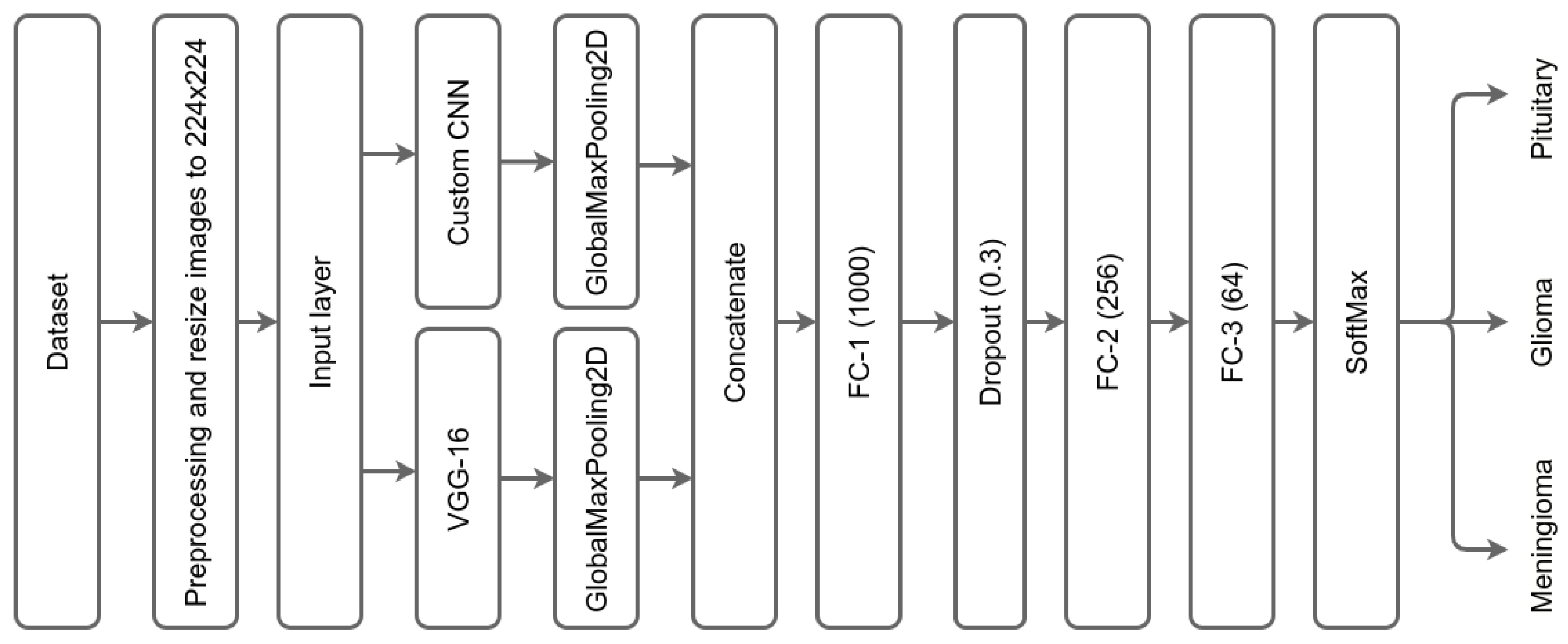
3.1. Dual Convolution Tumor Network (DCTN)
3.2. The DCTN Model Layers
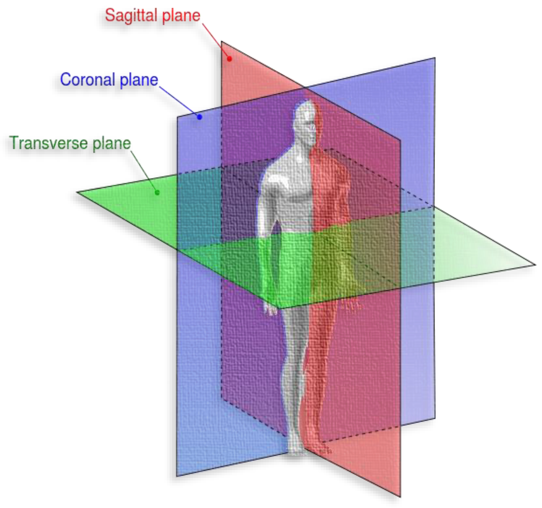
3.2.1. Image Input Layer
3.2.2. Convolution Layer
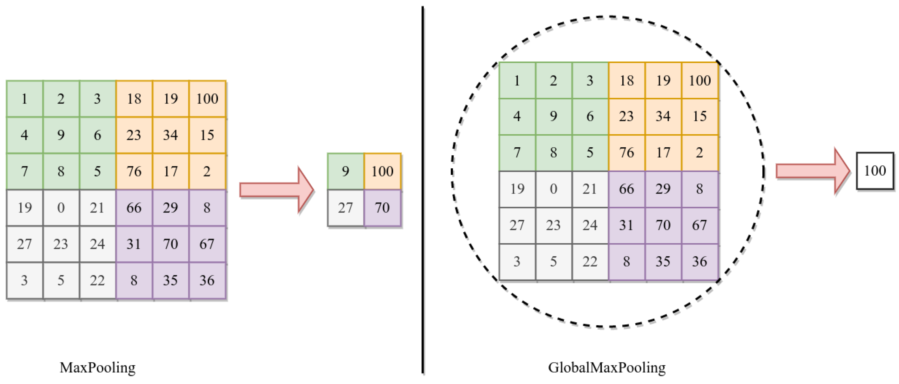
3.2.3. Pooling Layer
3.2.4. Fully Connected Layer
3.2.5. SoftMax Layer
3.2.6. Loss Function
3.3. DCTN Training Parameters
4. Dataset and Preprocessing
5. Results
Evaluation Metrics
6. Discussion
7. Conclusions and Future Work
Author Contributions
Funding
Institutional Review Board Statement
Informed Consent Statement
Data Availability Statement
Conflicts of Interest
References
- Mohta, S.; Sharma, S.; Saraya, A. Improvement in Adipocytic Indices as a Predictor of Improved Outcomes after TIPS: Right Conclusion? Liver Int. 2022, 42, 253. [Google Scholar] [CrossRef]
- Liu, Y.; Guo, Q.-F.; Chen, J.-L.; Li, X.-R.; Hou, F.; Liu, X.-Y.; Zhang, W.-J.; Zhang, Y.; Gao, F.-F.; Zhang, Y.-Z.; et al. Correlations between Alterations of T-Helper 17 Cells and Treatment Efficacy after Concurrent Radiochemotherapy in Locally Advanced Cervical Cancer (Stage IIB–IIIB): A 3-Year Prospective Study. Chin. Med. J. 2021, 134, 954–962. [Google Scholar] [CrossRef] [PubMed]
- Wong, M.C.S.; Huang, J.; Chan, P.S.F.; Choi, P.; Lao, X.Q.; Chan, S.M.; Teoh, A.; Liang, P. Global Incidence and Mortality of Gastric Cancer, 1980–2018. JAMA Netw. Open 2021, 4, e2118457. [Google Scholar] [CrossRef] [PubMed]
- Pang, L.; Khan, F.; Heimberger, A.B.; Chen, P. Mechanism and Therapeutic Potential of Tumor-Immune Symbiosis in Glioblastoma. Trends Cancer 2022, 8, 839–854. [Google Scholar] [CrossRef]
- Nelson, S.J. Multivoxel Magnetic Resonance Spectroscopy of Brain Tumors. Mol. Cancer Ther. 2003, 2, 497–507. [Google Scholar]
- Pfister, S.M.; Reyes-Múgica, M.; Chan, J.K.C.; Hasle, H.; Lazar, A.J.; Rossi, S.; Ferrari, A.; Jarzembowski, J.A.; Pritchard-Jones, K.; Hill, D.A.; et al. A Summary of the Inaugural WHO Classification of Pediatric Tumors: Transitioning from the Optical into the Molecular Era. Cancer Discov. 2021, 12, 331–355. [Google Scholar] [CrossRef] [PubMed]
- Ullah, N.; Khan, J.A.; Khan, M.S.; Khan, W.; Hassan, I.; Obayya, M.; Negm, N.; Salama, A.S. An Effective Approach to Detect and Identify Brain Tumors Using Transfer Learning. Appl. Sci. 2022, 12, 5645. [Google Scholar] [CrossRef]
- Chen, Y.; Schonlieb, C.-B.; Lio, P.; Leiner, T.; Dragotti, P.L.; Wang, G.; Rueckert, D.; Firmin, D.; Yang, G. AI-Based Reconstruction for Fast MRI—A Systematic Review and Meta-Analysis. Proc. IEEE 2022, 110, 224–245. [Google Scholar] [CrossRef]
- Keall, P.J.; Brighi, C.; Glide-Hurst, C.; Liney, G.; Liu, P.Z.Y.; Lydiard, S.; Paganelli, C.; Pham, T.; Shan, S.; Tree, A.C.; et al. Integrated MRI-Guided Radiotherapy—Opportunities and Challenges. Nat. Rev. Clin. Oncol. 2022, 19, 458–470. [Google Scholar] [CrossRef] [PubMed]
- Matheus, M.G.; Castillo, M.; Smith, J.K.; Armao, D.; Towle, D.; Muenzer, J. Brain MRI Findings in Patients with Mucopolysaccharidosis Types I and II and Mild Clinical Presentation. Neuroradiology 2004, 46, 666–672. [Google Scholar] [CrossRef]
- Singhal, A.B.; Topcuoglu, M.A.; Koroshetz, W.J. Diffusion MRI in Three Types of Anoxic Encephalopathy. J. Neurol. Sci. 2002, 196, 37–40. [Google Scholar] [CrossRef]
- Monté-Rubio, G.C.; Falcón, C.; Pomarol-Clotet, E.; Ashburner, J. A Comparison of Various MRI Feature Types for Characterizing Whole Brain Anatomical Differences Using Linear Pattern Recognition Methods. Neuroimage 2018, 178, 753–768. [Google Scholar] [CrossRef] [PubMed]
- Cheng, W.; Ping, Y.; Zhang, Y.; Chuang, K.-H.; Liu, Y. Magnetic Resonance Imaging (MRI) Contrast Agents for Tumor Diagnosis. J. Healthc. Eng. 2013, 4, 23–46. [Google Scholar] [CrossRef] [PubMed] [Green Version]
- Zacharaki, E.I.; Wang, S.; Chawla, S.; Soo Yoo, D.; Wolf, R.; Melhem, E.R.; Davatzikos, C. Classification of Brain Tumor Type and Grade Using MRI Texture and Shape in a Machine Learning Scheme. Magn. Reson. Med. 2009, 62, 1609–1618. [Google Scholar] [CrossRef] [PubMed] [Green Version]
- Khan, F.; Pang, L.; Dunterman, M.; Lesniak, M.S.; Heimberger, A.B.; Chen, P. Macrophages and Microglia in Glioblastoma: Heterogeneity, Plasticity, and Therapy. J. Clin. Investig. 2023, 133, 446–448. [Google Scholar] [CrossRef]
- Tandel, G.S.; Balestrieri, A.; Jujaray, T.; Khanna, N.N.; Saba, L.; Suri, J.S. Multiclass magnetic resonance imaging brain tumor classification using artificial intelligence paradigm. Comput. Biol. Med. J. 2020, 112, 103804. [Google Scholar] [CrossRef]
- Goyal, L.M.; Saba, T.; Rehman, A.; Larabi-Marie-Sainte, S. Artificial Intelligence and Internet of Things; CRC Press: Boca Raton, FL, USA, 2021. [Google Scholar]
- Jena, B.; Saxena, S.; Nayak, G.K.; Balestrieri, A.; Gupta, N.; Khanna, N.N.; Laird, J.R.; Kalra, M.K.; Fouda, M.M.; Saba, L.; et al. Brain Tumor Characterization Using Radiogenomics in Artificial Intelligence Framework. Cancers 2022, 14, 4052. [Google Scholar] [CrossRef]
- Di Cataldo, S.; Ficarra, E. Mining Textural Knowledge in Biological Images: Applications, Methods and Trends. Comput. Struct. Biotechnol. J. 2017, 15, 56–67. [Google Scholar] [CrossRef] [Green Version]
- Zhou, X.S.; Huang, T.S. CBIR: From Low-Level Features to High-Level Semantics. SPIE 2000, 3974, 426–431. [Google Scholar]
- Alzubaidi, L.; Duan, Y.; Al-Dujaili, A.; Ibraheem, I.K.; Alkenani, A.H.; Santamaría, J.; Fadhel, M.A.; Al-Shamma, O.; Zhang, J. Deepening into the Suitability of Using Pre-Trained Models of ImageNet against a Lightweight Convolutional Neural Network in Medical Imaging: An Experimental Study. PeerJ Comput. Sci. 2021, 7, e715. [Google Scholar] [CrossRef]
- Noreen, N.; Palaniappan, S.; Qayyum, A.; Ahmad, I.; Alassafi, M.O. Brain Tumor Classification Based on Fine-Tuned Models and the Ensemble Method. Comput. Mater. Contin. 2021, 67, 3967–3982. [Google Scholar] [CrossRef]
- Garg, G.; Garg, R. Brain Tumor Detection and Classification Based on Hybrid Ensemble Classifier. arXiv 2021, arXiv:2101.00216. [Google Scholar] [CrossRef]
- Shafi, A.; Rahman, M.B.; Anwar, T.; Halder, R.S.; Kays, H.E. Classification of Brain Tumors and Auto-Immune Disease Using Ensemble Learning. Inform. Med. Unlocked 2021, 24, 100608. [Google Scholar] [CrossRef]
- Jena, B.; Nayak, G.K.; Saxena, S. An Empirical Study of Different Machine Learning Techniques for Brain Tumor Classification and Subsequent Segmentation Using Hybrid Texture Feature. Mach. Vis. Appl. 2022, 33, 6. [Google Scholar] [CrossRef]
- Ahsan, A.; Muhammad, A.; Usman, T.; Yunyoung, N.; Muhammad, N.; Chang-Won, J.; Reham, R.M.; Rasha, H.S. An Ensemble of Optimal Deep Learning Features for Brain Tumor Classification. CMC-Comput. Mater. Contin. 2021, 69, 2653–2670. [Google Scholar] [CrossRef]
- Zahoor, M.M.; Qureshi, S.A.; Bibi, S.; Khan, S.H.; Khan, A.; Ghafoor, U.; Bhutta, M.R. A New Deep Hybrid Boosted and Ensemble Learning-Based Brain Tumor Analysis Using MRI. Sensors 2022, 22, 2726. [Google Scholar] [CrossRef] [PubMed]
- Benyuan, S.; Jinqiao, D.; Zihao, L.; Cong, L.; Yi, Y.; Bo, B. GPPF: A General Perception Pre-Training Framework via Sparsely Activated Multi-Task Learning. arXiv 2022, arXiv:2208.02148. [Google Scholar] [CrossRef]
- Han, K.; Xiao, A.; Wu, E.; Enhua, J.; Xu, C.; Wang, Y. Transformer in Transformer. Adv. Neural Inf. Process. Syst. 2021, 34, 15908–15919. [Google Scholar]
- Wang, W.; Chen, C.; Ding, D.; Yu, H.; Zha, S.; Li, J. Transbts: Multimodal Brain Tumor Segmentation Using Transformer. In Proceedings of the Medical Image Computing and Computer Assisted Intervention–MICCAI 2021: 24th International Conference, Strasbourg, France, 27 September–1 October 2021; Springer: Berlin/Heidelberg, Germany, 2021; pp. 109–119. [Google Scholar]
- Yurong, G.; Muhammad, A.; Ziaur, R.; Ammara, A.; Waheed Ahmed, A.; Zaheer Ahmed, D.; Muhammad Shoaib, B.; Zhihua, H. A Framework for Efficient Brain Tumor Classification Using MRI Images. Math. Biosci. Eng. 2021, 18, 5790–5815. [Google Scholar]
- Zhang, S.; Yuan, G.-C. Deep Transfer Learning for COVID-19 Detection and Lesion Recognition Using Chest CT Images. Comput. Math. Methods Med. 2022, 2022, 4509394. [Google Scholar] [CrossRef]
- Ansari, S.U.; Javed, K.; Qaisar, S.M.; Jillani, R.; Haider, U. Multiple Sclerosis Lesion Segmentation in Brain MRI Using Inception Modules Embedded in a Convolutional Neural Network. J. Healthc. Eng. 2021, 2021, 4138137. [Google Scholar] [CrossRef] [PubMed]
- Andrearczyk, V.; Oreiller, V.; Hatt, M.; Depeursinge, A. Head and Neck Tumor Segmentation and Outcome Prediction: Second Challenge, HECKTOR 2021, Held in Conjunction with MICCAI 2021, Strasbourg, France, 27 September 2021, Proceedings; Springer: Cham, Switzerland, 2022.
- Ranjbarzadeh, R.; Bagherian Kasgari, A.; Jafarzadeh Ghoushchi, S.; Anari, S.; Naseri, M.; Bendechache, M. Brain Tumor Segmentation Based on Deep Learning and an Attention Mechanism Using MRI Multi-Modalities Brain Images. Sci. Rep. 2021, 11, 10930. [Google Scholar] [CrossRef] [PubMed]
- Ismail, A.; Abdlerazek, S.; El-Henawy, I.M. Development of smart healthcare system based on speech recognition using support vector machine and dynamic time warping. Sustainability 2020, 12, 2403. [Google Scholar] [CrossRef] [Green Version]
- Lhotska, L.; Sukupova, L.; Lacković, I.; Ibbott, G.S. World Congress on Medical Physics and Biomedical Engineering 2018: June 3–8, 2018, Prague, Czech Republic (Vol.1); Springer: Singapore, 2019. [Google Scholar]
- Munir, K.; Frezza, F.; Rizzi, A. Deep Learning Hybrid Techniques for Brain Tumor Segmentation. Sensors 2022, 22, 8201. [Google Scholar] [CrossRef] [PubMed]
- Gómez-Guzmán, M.A.; Jiménez-Beristaín, L.; García-Guerrero, E.E.; López-Bonilla, O.R.; Tamayo-Perez, U.J.; Esqueda-Elizondo, J.J.; Palomino-Vizcaino, K.; Inzunza-González, E. Classifying Brain Tumors on Magnetic Resonance Imaging by Using Convolutional Neural Networks. Electronics 2023, 12, 955. [Google Scholar] [CrossRef]
- Gull, S.; Akbar, S.; Khan, H.U. Automated Detection of Brain Tumor through Magnetic Resonance Images Using Convolutional Neural Network. BioMed Res. Int. 2021, 2021, 3365043. [Google Scholar] [CrossRef]
- Latif, G.; Ben Brahim, G.; Iskandar, D.N.F.A.; Bashar, A.; Alghazo, J. Glioma Tumors’ Classification Using Deep-Neural-Network-Based Features with SVM Classifier. Diagnostics 2022, 12, 1018. [Google Scholar] [CrossRef]
- Díaz-Pernas, F.J.; Martínez-Zarzuela, M.; Antón-Rodríguez, M.; González-Ortega, D. A Deep Learning Approach for Brain Tumor Classification and Segmentation Using a Multiscale Convolutional Neural Network. Healthcare 2021, 9, 153. [Google Scholar] [CrossRef]
- Dequidt, P.; Bourdon, P.; Tremblais, B.; Guillevin, C.; Gianelli, B.; Boutet, C.; Cottier, J.-P.; Vallée, J.-N.; Fernandez-Maloigne, C.; Guillevin, R. Exploring Radiologic Criteria for Glioma Grade Classification on the BraTS Dataset. IRBM 2021, 42, 407–414. [Google Scholar] [CrossRef]
- Abd El Kader, I.; Xu, G.; Shuai, Z.; Saminu, S.; Javaid, I.; Salim Ahmad, I. Differential Deep Convolutional Neural Network Model for Brain Tumor Classification. Brain Sci. 2021, 11, 352. [Google Scholar] [CrossRef]
- Cheng, J.; Huang, W.; Cao, S.; Yang, R.; Yang, W.; Yun, Z.; Wang, Z.; Feng, Q. Correction: Enhanced Performance of Brain Tumor Classification via Tumor Region Augmentation and Partition. PLoS ONE 2015, 10, e0144479. [Google Scholar] [CrossRef] [PubMed]
- Jiang, Z.; Dong, Z.; Wang, L.; Jiang, W. Method for Diagnosis of Acute Lymphoblastic Leukemia Based on ViT-CNN Ensemble Model. Comput. Intell. Neurosci. 2021, 2021, 7529893. [Google Scholar] [CrossRef] [PubMed]
- Ali, M.B.; Gu, I.Y.-H.; Berger, M.S.; Pallud, J.; Southwell, D.; Widhalm, G.; Roux, A.; Vecchio, T.G.; Jakola, A.S. Domain Mapping and Deep Learning from Multiple MRI Clinical Datasets for Prediction of Molecular Subtypes in Low Grade Gliomas. Brain Sci. 2020, 10, 463. [Google Scholar] [CrossRef] [PubMed]
- Rehman, H.Z.U.; Hwang, H.; Lee, S. Conventional and Deep Learning Methods for Skull Stripping in Brain MRI. Appl. Sci. 2020, 10, 1773. [Google Scholar] [CrossRef] [Green Version]
- Mahmoud, A.T.; Awad, W.A.; Behery, G.; Abouhawwash, M.; Masud, M.; Aljuaid, H.; Ebada, A.I. An Automatic Deep Neural Network Model for Fingerprint Classification. Intell. Autom. Soft Comput. 2023, 36, 2007–2023. [Google Scholar] [CrossRef]
- Rathore, S.; Niazi, T.; Iftikhar, M.A.; Chaddad, A. Glioma Grading via Analysis of Digital Pathology Images Using Machine Learning. Cancers 2020, 12, 578. [Google Scholar] [CrossRef] [Green Version]
- Shaver, M.M.; Kohanteb, P.A.; Chiou, C.; Bardis, M.D.; Chantaduly, C.; Bota, D.; Filippi, C.G.; Weinberg, B.; Grinband, J.; Chow, D.S.; et al. Optimizing Neuro-Oncology Imaging: A Review of Deep Learning Approaches for Glioma Imaging. Cancers 2019, 11, 829. [Google Scholar] [CrossRef] [Green Version]
- Shen, Y.; Ma, Y.; Deng, S.; Huang, C.-J.; Kuo, P.-H. An Ensemble Model based on Deep Learning and Data Pre-processing for Short-Term Electrical Load Forecasting. Sustainability 2021, 13, 1694. [Google Scholar] [CrossRef]
- Riva, M.; Sciortino, T.; Secoli, R.; D’Amico, E.; Moccia, S.; Fernandes, B.; Conti Nibali, M.; Gay, L.; Rossi, M.; De Momi, E.; et al. Glioma biopsies Classification Using Raman Spectroscopy and Machine Learning Models on Fresh Tissue Samples. Cancers 2021, 13, 1073. [Google Scholar] [CrossRef]
- Kim, H.; Jeong, Y.S. Sentiment Classification Using Convolutional Neural Networks. Appl. Sci. 2019, 9, 2347. [Google Scholar] [CrossRef] [Green Version]
- Pal, K.; Mitra, K.; Bit, A.; Bhattacharyya, S.; Dey, A. Medical Signal Processing in Biomedical and Clinical Applications. J. Healthc. Eng. 2018, 2018, 3932471. [Google Scholar] [CrossRef]
- Bumes, E.; Wirtz, F.-P.; Fellner, C.; Grosse, J.; Hellwig, D.; Oefner, P.J.; Häckl, M.; Linker, R.; Proescholdt, M.; Schmidt, N.O.; et al. Non-Invasive Prediction of IDH Mutation in Patients with Glioma WHO II/III/IV Based on F-18-FET PET-Guided In Vivo 1H-Magnetic Resonance Spectroscopy and Machine Learning. Cancers 2020, 12, 3406. [Google Scholar] [CrossRef]
- BT. Data Set. Available online: https://figshare.com/articles/dataset/brain_tumor_dataset/1512427 (accessed on 16 April 2023).
- 1.2D: Body Planes and Sections. Medicine LibreTexts. Available online: https://med.libretexts.org/Courses/Okanagan_College/HKIN_110%3A_Human_Anatomy_I_for_Kinesiology/01%3A_Introduction_to_Anatomy/1.02%3A_Mapping_the_Body/1.2D%3A_Body_Planes_and_Sections (accessed on 16 April 2023).
- Nwankpa, C.; Ijomah, W.; Gachagan, A.; Marshall, S. Activation Functions: Comparison of Trends in Practice and Research for Deep Learning. arXiv 2018, arXiv:1811.03378. [Google Scholar] [CrossRef]
- Yaqub, M.; Feng, J.; Zia, M.S.; Arshid, K.; Jia, K.; Rehman, Z.U.; Mehmood, A. State-of-the-Art CNN Optimizer for Brain Tumor Segmentation in Magnetic Resonance Images. Brain Sci. 2020, 10, 427. [Google Scholar] [CrossRef] [PubMed]
- Ghaffari, M.; Sowmya, A.; Oliver, R. Automated Brain Tumour Segmentation Using Multimodal Brain Scans, a Survey Based on Models Submitted to the BraTS 2012–2018 Challenges. IEEE Rev. Biomed. Eng. 2019, 13, 156–168. [Google Scholar] [CrossRef] [PubMed]
- Rani, G.; Tiwari, P.K. Handbook of Research on Disease Prediction through Data Analytics and Machine Learning; IGI Global, Medical Information Science Reference: Hershey, PA, USA, 2021. [Google Scholar]
- Deepak, S.; Ameer, P.M. Brain Tumor Classification Using Deep CNN Features via Transfer Learning. Comput. Biol. Med. 2019, 111, 103345. [Google Scholar] [CrossRef] [PubMed]
- Zulfiqar, F.; Ijaz Bajwa, U.; Mehmood, Y. Multiclass Classification of Brain Tumor Types from MR Images Using EfficientNets. Biomed. Signal Process. Control 2023, 84, 104777. [Google Scholar] [CrossRef]
- Zahoor, M.M.; Khan, S.H. Brain Tumor MRI Classification Using a Novel Deep Residual and Regional CNN. arXiv 2022, arXiv:2211.16571. [Google Scholar] [CrossRef]
- Verma, A.; Singh, V.P. Design, Analysis and Implementation of Efficient Deep Learning Frameworks for Brain Tumor Classification. Multimed. Tools Appl. 2022, 81, 37541–37567. [Google Scholar] [CrossRef]
- Vidyarthi, A.; Agarwal, R.; Gupta, D.; Sharma, R.; Draheim, D.; Tiwari, P. Machine Learning Assisted Methodology for Multiclass Classification of Malignant Brain Tumors. IEEE Access 2022, 10, 50624–50640. [Google Scholar] [CrossRef]
- Molder, C.; Lowe, B.; Zhan, J. Learning Medical Materials from Radiography Images. Front. Artif. Intell. 2021, 4, 638299. [Google Scholar] [CrossRef] [PubMed]
- Yerukalareddy, D.R.; Pavlovskiy, E. Brain Tumor Classification Based on Mr Images Using GAN as a Pre-Trained Model. In Proceedings of the 2021 IEEE Ural-Siberian Conference on Computational Technologies in Cognitive Science, Genomics and Biomedicine (CSGB), Yekaterinburg, Russia, 26–28 May 2021; IEEE: Piscataway, NJ, USA, 2021; pp. 380–384. [Google Scholar]
- Hilles, S.M.S.; Saleh, N.S. Image Segmentation and Classification Using CNN Model to Detect Brain Tumors. In Proceedings of the 2021 2nd International Informatics and Software Engineering Conference (IISEC), Ankara, Turkey, 16–17 December 2021; IEEE: Piscataway, NJ, USA, 2021; pp. 1–7. [Google Scholar]
- Chaki, J.; Woźniak, M. A Deep Learning Based Four-Fold Approach to Classify Brain MRI: BTSCNet. Biomed. Signal Process. Control 2023, 85, 104902. [Google Scholar] [CrossRef]


| Layer | Input Size | No. Filters | Kernel Size | Stride | |
|---|---|---|---|---|---|
| VGG-16 | Conv1-1 | 224 × 224 | 64 | 3 × 3 | 2 |
| Conv1-2 | 224 × 224 | 64 | 3 × 3 | ||
| Maxpool | 2 × 2 | 2 | |||
| Conv2-1 | 112 × 112 | 128 | 3 × 3 | 2 | |
| Conv2-2 | 112 × 112 | 128 | 3 × 3 | 2 | |
| Maxpool | 2 × 2 | 2 | |||
| Conv3-1 | 56 × 56 | 256 | 3 × 3 | 2 | |
| Conv3-2 | 56 × 56 | 256 | 3 × 3 | 2 | |
| Conv3-3 | 56 × 56 | 256 | 3 × 3 | 2 | |
| Maxpool | 2 × 2 | 2 | |||
| Conv4-1 | 28 × 28 | 512 | 3 × 3 | 2 | |
| Conv4-2 | 28 × 28 | 512 | 3 × 3 | 2 | |
| Conv4-3 | 28 × 28 | 512 | 3 × 3 | 2 | |
| Maxpool | 2 × 2 | 2 | |||
| Conv5-1 | 14 × 14 | 512 | 3 × 3 | 2 | |
| Conv5-2 | 14 × 14 | 512 | 3 × 3 | 2 | |
| Conv5-3 | 14 × 14 | 512 | 3 × 3 | 2 | |
| Maxpool | 2 × 2 | 2 | |||
| Layer | Input Size | No. Filters | Kernel Size | Stride | |
|---|---|---|---|---|---|
| Custom CNN | Conv1-1 | 224 × 224 | 7 | 3 × 3 | 1 |
| Conv1-2 | 224 × 224 | 9 | 3 × 3 | 1 | |
| Maxpool | 2 × 2 | 2 | |||
| Conv2-1 | 112 × 112 | 16 | 3 × 3 | 1 | |
| Conv2-2 | 112 × 112 | 32 | 3 × 3 | 1 | |
| Maxpool | 2 × 2 | 2 | |||
| Conv3-1 | 56 × 56 | 32 | 3 × 3 | 1 | |
| Conv3-2 | 56 × 56 | 64 | 3 × 3 | 1 | |
| Maxpool | 2 × 2 | 2 | |||
| Conv4-1 | 28 × 28 | 64 | 3 × 3 | 1 | |
| Conv4-2 | 28 × 28 | 64 | 3 × 3 | 1 | |
| Maxpool | 2 × 2 | 2 | |||
| Conv5-1 | 14 × 14 | 64 | 3 × 3 | 1 | |
| Conv5-2 | 14 × 14 | 128 | 3 × 3 | 1 | |
| Conv5-1 | 7 × 7 | 128 | 3 × 3 | 1 | |
| Conv5-2 | 7 × 7 | 128 | 3 × 3 | 1 | |
| Maxpool | 2 × 2 | 2 | |||
| Parameters | Value |
|---|---|
| Initial learning rate | 0.0001 |
| Batch size | 64 |
| No. of epochs | 50 |
| Shuffle | every epoch |
| Loss function | Sparse-categorical-cross-entropy |
| Tumor Type | Coronal | Axial | Sagittal | Total |
|---|---|---|---|---|
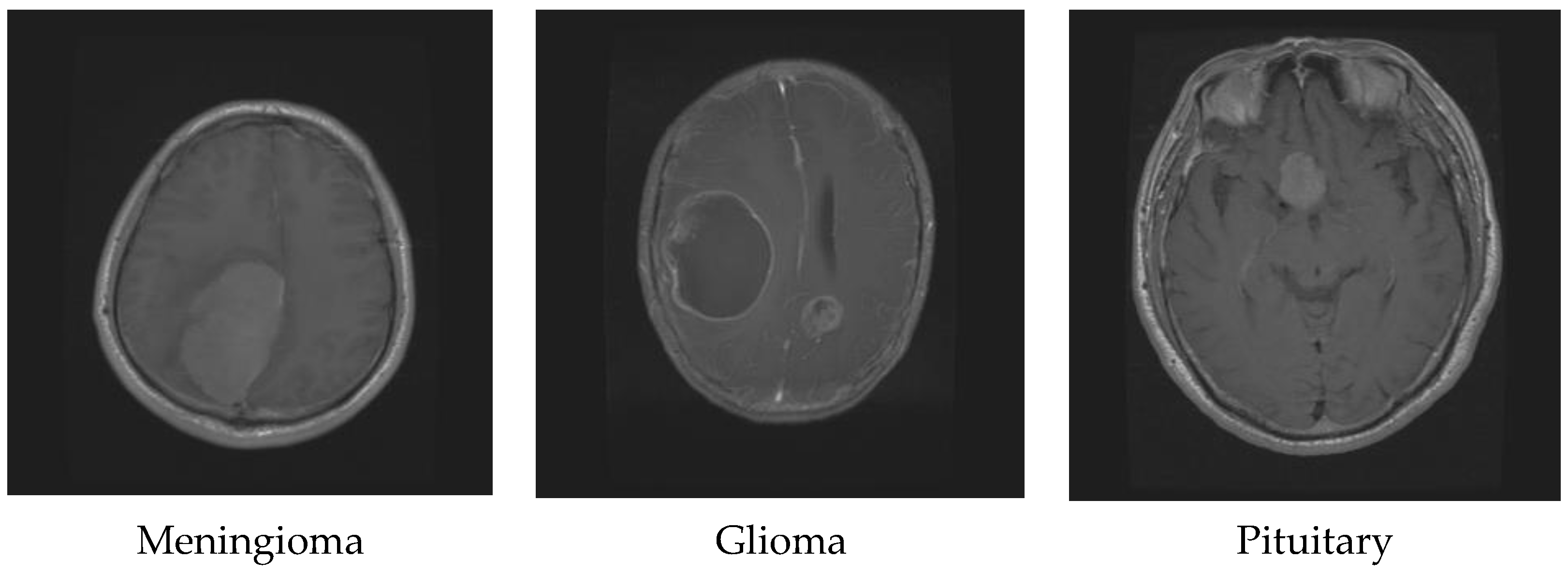
| Meningioma | 268 | 209 | 231 | 708 |
| Glioma | 437 | 494 | 495 | 1426 |
| Pituitary | 319 | 291 | 320 | 930 |
| Total | 3064 |
| Precision | Recall | F1-Score | Support | |
|---|---|---|---|---|
| Meningioma | 0.99 | 0.98 | 0.98 | 134 |
| Glioma | 0.99 | 1.00 | 0.99 | 286 |
| Pituitary | 0.98 | 0.99 | 0.99 | 193 |
| Accuracy | 0.99 | 613 | ||
| Macro avg | 0.99 | 0.99 | 0.99 | 613 |
| Weighted avg | 0.99 | 0.99 | 0.99 | 613 |
| Method | Classification Type | Used Technique | Accuracy |
|---|---|---|---|
| In Ref. [63] | Multiclass (Glioma, Meningioma, and Pituitary Tumor) | CNN, Transfer learning (Google Net) | 98% |
| In Ref. [64] | Multiclass (Glioma, Meningioma, and Pituitary Tumor) | CNN, Fine-tuned EfficientNetB2 | 98.86% |
| In Ref. [65] | Multiclass (Glioma, Meningioma, and Pituitary Tumor, Healthy Images) | Novel deep residual and regional-based Res-BRNet convolutional neural network (CNN) | 98.22% |
| In Ref. [66] | Multiclass (Glioma, Meningioma, and Pituitary Tumor) | DenseNet201-based transfer learning MobileNet | 98.22% 97.87% |
| In Ref. [67] | Binary-Classification (Malignant and Non-Malignant) | K-nearest neighbor (KNN) multiclass support vector machine (MSVM) neural network (NN) | 88.43% 92.5% 95.86% |
| In Ref. [68] | Multiclass (Glioma, Meningioma, and Pituitary Tumor) | A siamese neural network called D-CNN, material recognition neural networks (MAC-CNN) | 92.8% |
| In Ref. [69] | Multiclass (Glioma, Meningioma, Pituitary Tumor, and non-tumor) | Generative adversarial network (GAN), multiscale gradient GAN (MSGGAN) with auxiliary classification | 98.57% |
| In Ref. [70] | Multi-Class (Glioma, Meningioma, and Pituitary Tumor) | CNN, cross-validation technique | 96.56% |
| In Ref. [42] | Multiclass (Glioma, Meningioma, and Pituitary Tumor) | CNN includes a multiscale approach | 97.3% |
| In Ref. [71] | Multiclass (Glioma, Meningioma, and Pituitary Tumor) | Brain tumor segmentation and classification network (BTSCNet) | Meningioma 96.6% (using MR-Contrast feature) Glioma 98.1% (using MR-Correlation feature) Pituitary 95.3% (using MR-Homogeneity feature) |
| Proposed Model | Multiclass (Glioma, Meningioma, and Pituitary Tumor) | Dual CNN (VGG16, Custom CNN) | 99% |
Disclaimer/Publisher’s Note: The statements, opinions and data contained in all publications are solely those of the individual author(s) and contributor(s) and not of MDPI and/or the editor(s). MDPI and/or the editor(s) disclaim responsibility for any injury to people or property resulting from any ideas, methods, instructions or products referred to in the content. |
© 2023 by the authors. Licensee MDPI, Basel, Switzerland. This article is an open access article distributed under the terms and conditions of the Creative Commons Attribution (CC BY) license (https://creativecommons.org/licenses/by/4.0/).
Share and Cite
Al-Zoghby, A.M.; Al-Awadly, E.M.K.; Moawad, A.; Yehia, N.; Ebada, A.I. Dual Deep CNN for Tumor Brain Classification. Diagnostics 2023, 13, 2050. https://doi.org/10.3390/diagnostics13122050
Al-Zoghby AM, Al-Awadly EMK, Moawad A, Yehia N, Ebada AI. Dual Deep CNN for Tumor Brain Classification. Diagnostics. 2023; 13(12):2050. https://doi.org/10.3390/diagnostics13122050
Chicago/Turabian StyleAl-Zoghby, Aya M., Esraa Mohamed K. Al-Awadly, Ahmad Moawad, Noura Yehia, and Ahmed Ismail Ebada. 2023. "Dual Deep CNN for Tumor Brain Classification" Diagnostics 13, no. 12: 2050. https://doi.org/10.3390/diagnostics13122050