1. Introduction
Hypoxia is a condition that occurs when there is a reduced oxygen supply to the body’s tissues, while birth asphyxia is oxygen deprivation that happens around the time of birth due to various perinatal events [
1]. Hypoxia can result in a spectrum of acid–base changes and physiological disorders at the cellular, tissue, or organ level [
2]. The global annual burden of this disease is about four million cases, leading to one million neonatal deaths [
3]. Birth asphyxia and subsequent metabolic acidosis (neonatal acidemia) are also associated with early neonatal death, which is defined as the death of a newborn between zero and seven days after birth, and it accounts for 73% of all postnatal deaths worldwide. Additionally, birth asphyxia can lead to multiorgan dysfunction, hypoxic–ischemic encephalopathy, seizures, cerebral palsy, long-term neurological sequelae, and neonatal mortality [
4].
Arterial blood gas (ABG) analysis is considered essential for the accurate diagnosis and clinical management of birth asphyxia [
5]. ABG is a diagnostic tool for measuring oxygen, carbon dioxide, and acid–base disorder in the blood [
5]. In ABG analysis, blood is the primary source for identifying biomarkers for the accurate diagnosis of asphyxia [
6]. Neonatal blood sampling requires skilled handling to ensure sufficient sample acquisition while also minimizing the risk of complications such as bleeding, infection, and vascular damage due to the small size and fragility of blood vessels. Additionally, the limited volume of blood that can be safely obtained from neonates increases the difficulty of sampling, necessitating careful selection of appropriate tests and techniques to avoid unnecessary patient discomfort or harm [
7,
8]. Despite ABG’s potential clinical advantages, the non-continuous mode and discomfort associated with invasive blood sampling are the key drawbacks of ABG [
6]. As an alternative to blood, interstitial fluid (ISF) is a more sensitive physiological indicator of asphyxia. Mild metabolic disorders can be effectively buffered by blood, which helps maintain arterial blood pH within the normal range [
9]. However, due to the limited buffering capacity of ISF, pH levels quickly change in response to hypoxic events, making ISF more susceptible to even small changes in pH levels resulting from severe hypoxia. This can cause significant deviations from the normal pH range in the ISF [
9]. In the last two decades, ISF has been used for minimally invasive detection of various health conditions such as hereditary metabolic disorders, organ failure, and therapeutic efficacy [
9]. Additionally, ISF’s composition is similar to that of blood due to the equilibrium maintained by small molecules, such as carbon dioxide, phosphates, and albumin. This similarity in composition makes ISF an interesting alternative to blood analysis for clinical applications, as it allows for non-invasive sampling while maintaining the same physiological outputs [
10]. Due to ISF’s advantages in terms of volume and composition, ISF is a promising alternative for continuous sampling and monitoring of hypoxia-associated metabolic disorders and asphyxia [
11].
Various techniques have been developed for the extraction of ISF from the skin, including suction blisters, open-flow microperfusion, and microdialysis [
12]. However, these techniques can be complicated, require trained professionals, and use bulky instruments that may cause discomfort to patients [
13]. In contrast, microneedle patches are a minimally invasive, continuous, rapid, and cost-effective technology that overcomes the challenges associated with dermal ISF sampling [
14]. The reduced invasiveness of ISF sampling and the sensitivity of ISF to severe hypoxia (asphyxia) and metabolic disorders compared to blood makes ISF an attractive target for biosensor-based detection of asphyxia in a minimally invasive manner [
11]. To develop these sensors, researchers require physiologically representative liquid samples that mimic the properties of ISF. This need is particularly critical for the development of a universal biosensor for continuous and minimally invasive asphyxia monitoring. ISF-mimicking solutions could provide a simple and rapid solution for the pre-clinical testing and validation of continuous asphyxia-monitoring biosensors.
pH, as a quantitative measure of solution acidity or alkalinity, plays a crucial role in predicting asphyxia. Low pH levels (acidosis (pH < 7.30)) reliably indicate the occurrence of asphyxia, whereas high pH levels signify the occurrence of metabolic alkalosis (pH > 7.45) [
15], potentially arising from inadequate management of oxygen supply during asphyxia interventions [
16]. Monitoring pH levels in bodily fluids such as ISF can provide healthcare professionals with valuable insights into the severity and progression of asphyxia, facilitating accurate diagnosis and treatment decisions [
17]. The pH of body fluids has been thoroughly investigated, and an average value of pH 7.4 is generally reported [
18]. However, the pH of ISF and its variability have not been well investigated in the literature. The majority of published evidence indicates that under healthy settings, the pH of ISF is similar to the pH of blood, i.e., 7.35–7.45 [
18,
19]. ISF-mimicking solutions could support the design of initial systems of biosensors for in vivo dermal ISF by enabling an understanding of the variables influencing the system’s quality and performance [
20].
The objective of this study was to develop ISF-mimicking solutions with the same pH as normal ISF, as well as hypoxic ISF characterized by acidosis or alkalosis. In addition, this study aimed to investigate the relationship between the pH of ISF and its electrical properties, including impedance and conductivity, under normal and hypoxic conditions. This work allows for the subsequent development and testing of an impedance-based biosensor for the detection of hypoxia-induced pH changes in ISF. A series of buffer solutions were prepared with varying pH ranges, and their electrical properties were characterized by measuring their impedance using a four-probe method. The impedance data were then converted to conductivity data, and eight mimicking solutions were selected based on their electrical conductivity values falling within the required conductivity range (0.41–0.80 S/m) of ISF. The experimental procedure began with the measurements of the pH and impedance of the buffers at their actual pH values to observe acidosis without any adjustments made to the pH levels. Subsequently, hypoxic acidosis was induced by adding hydrochloric acid (HCl). Following this, alkalosis was observed without adjusting the pH values of the buffers. Finally, the addition of sodium hydroxide (NaOH) was used to observe the effect of alkalosis in the buffering solution. The process of selecting the most appropriate buffers to mimic ISF involved evaluating their pH values, pH–impedance plots, and conductivity across a frequency range of 10 Hz to 100 kHz. This selection was made by comparing the properties of various buffers and choosing the ones that exhibited the closest resemblance to ISF.
2. Materials and Methods
2.1. Selection of Mimicking Materials
In this study, a range of buffers were prepared with pH values ranging from 6 to 8. This range of pH mimics the impact of severe-hypoxia-induced acidosis and poor-hypoxia-management-induced alkalosis. The buffer systems and their corresponding pH ranges are tabulated in
Table 1.
The selection of a buffer for the preparation of ISF-mimicking solutions is primarily determined by the pH value of the buffer, which serves as the fundamental characteristic defining its capacity to maintain a stable pH environment [
15]. Other key parameters include the buffer capacity or pKa value, the solubility of the buffer in water, temperature, and the concentration and ionic strength of its components [
19]. Optimal buffering is achieved when the pH value of the buffer system is within one unit of its pKa value, which can be expressed mathematically by Equation (1) [
21]:
In addition to pH, other factors including the stability and nature of the buffer are also considered in selecting appropriate buffers. For instance, although imidazole-HCl buffer has a pH range of 6.2–7.8, it tends to bind with various metals and is largely unstable [
22]. Moreover, when creating buffers in the laboratory, the hazardous nature of the buffer is also taken into account [
23]. Cacodylate, for instance, is a hazardous buffer that, when combined with a low pH value, can lead to enzyme inactivation [
23]. Despite these challenges, all prepared buffers and reagents are commercially available and have a relatively low cost.
A simple and effective method for determining whether an aqueous solution of a conjugate acid/base pair functions as a buffer is the use of the Henderson–Hasselbalch Equation (2) [
24]:
where Ka is the acid disassociation constant, pKa is the negative logarithm of Ka, HA is the concentration of the acid, and A
− is the concentration of the conjugate base. This equation allows for the calculation of the acidity of the buffer solution by considering the pKa of the acid and the ratio of the concentrations of the conjugate acid and base forms of the buffer.
The pH of interstitial fluid (ISF) is a critical clinical biomarker for determining asphyxia in neonates and ISF phantom design due to its rapid response to metabolic disturbances, clinical relevance, and specificity for acidosis assessment [
16,
25]. Furthermore, pH is a primary factor influencing electrical conductivity, which is essential for developing and testing impedance-based sensors for asphyxia detection [
26,
27]. While carbon dioxide (CO
2) and oxygen (O
2) levels are also important in assessing neonatal asphyxia, pH is considered more critical because it provides a comprehensive view of the overall acid–base status of the infant. It reflects not only the degree of respiratory distress (as indicated by CO
2 levels) but also the metabolic consequences of oxygen deprivation (as indicated by lactate accumulation) [
15,
16]. Therefore, in this study, pH is prioritized as the primary biomarker in the development of electrical conductivity/impedance-based ISF phantoms.
2.2. Preparation of Buffers
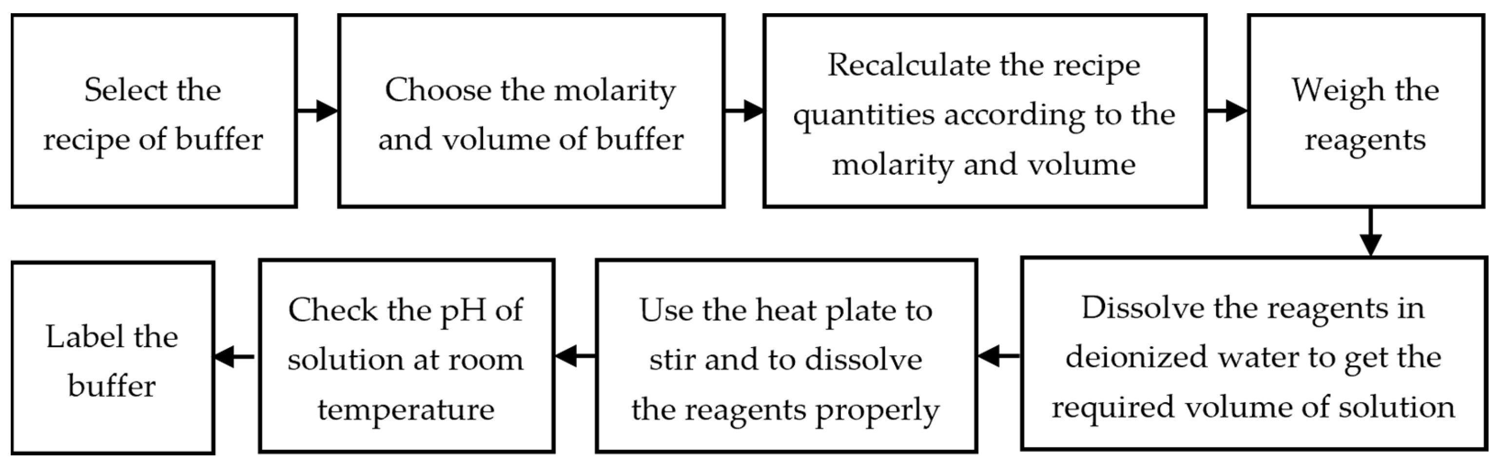
Henderson and Hasselbalch’s equation (Equation (2)) was used to make buffered solutions by determining the precise amounts of acid and base required to achieve the desired pH [
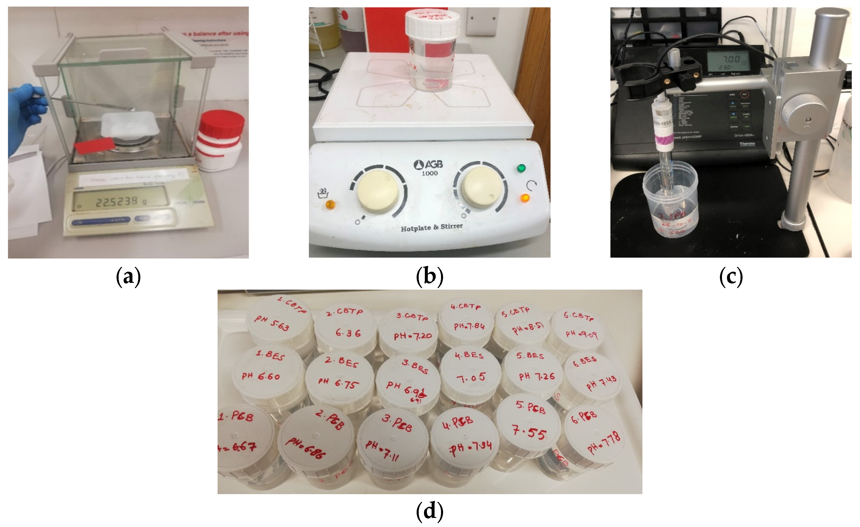
24]. The preparation of a buffer involves several steps, including weighing the chemical reagents with high precision and accuracy of the weighing scale, dissolving them in de-ionized water, and measuring the resultant pH with the calibrated and accurate pH meter (Thermo Electron Corporation 420A+, Waltham, MA, USA).
The flow sheet diagram of the stepwise process of the preparation of the buffers is shown in
Figure 1 and
Figure 2. Because the acid-to-base ratio in a buffer is directly tied to the resulting pH, it is critical to utilize precision and accuracy when preparing a buffer by utilizing equipment such as a weighing scale, pipets, and a pH meter [
28]. For accurately weighing the chemical reagents, an analytical balance (Mettler Toledo AB54, Columbus, OH, USA) with a readability of 0.1 mg and repeatability of 0.08 mg was used. Before measuring each chemical reagent, the weighing container or paper was cleared by placing the container on top of the balance, effectively canceling out its weight and establishing a zero-reference point. The pH meter was used to record the pH values of each buffer solution. The pH meter was calibrated with standard calibrated pH solutions (pH = 4.00, pH = 7.00, pH = 10.00). These standard buffer solutions with a tolerance of ±0.02 pH units were purchased from Fischer Scientific, Dublin, Ireland. The pH sensor was cleaned with de-ionized water and was dried before each measurement.
The concentrations of most buffers that operate optimally are between 0.1 M and 10 M. When preparing the buffer solution, to keep consistency throughout the experiment, the concentration of each buffer solution was kept constant, 0.1 M, and the total volume of the buffered solution was 0.1 L. HCl and NaOH were used to introduce the effects of metabolic acidosis and metabolic alkalosis, respectively.
The conductivity of all the buffers was calculated from the recorded impedance values. As the conductivity values are temperature-dependent, to provide a consistent point of reference for comparison, standard conditions were established at room temperature, which is typically defined as 22 ± 3 °C. All the measurements were completed at room temperature, and the temperature of each buffer was measured by using a digital thermometer with a resolution of 0.01 pH units and an accuracy of ±0.005 units.
If the buffers were required to be prepared by mixing the stock solution, the required mass of the reagents to prepare the stock solution was calculated by using Equations (3) and (4) [
29].
where
= molar weight or molar weight (g/mol),
= mass of the substance in grams (g), and
= number of moles of a substance.
where
= molar concentration/molarity (mol/L),
= moles of the solute (mol), and
= final volume of the solution (L). The concentration of resulting solutions using stock solutions can be determined by using Equations (5) and (6) as follows:
where
= stock solution’s concentration,
= volume of stock solution,
= dilute solution’s concentration, and
= volume of the dilute solution. The buffers are prepared at different pH values and are described with their reagents in
Table 2.
2.3. Measurement Setup
Two types of measurements were performed on each buffer solution. The pH of each buffer solution was measured using a digital pH meter (Orion model 420Aplus, Thermo Fischer Scientific, Waltham, MA, USA) and a mercury-free pH combination electrode (Thermo Fischer Scientific, Waltham, MA, USA). Before the measurements, the pH meter was calibrated using standard buffers of pH 4.0, 7.0, and 10.0. After allowing the reading to stabilize for 30 s, the pH was recorded. The temperature was also recorded using a digital thermometer (Hanna Instruments, Smithfield, RI, USA, model 1204, Thermo Fischer Scientific, Waltham, MA, USA).
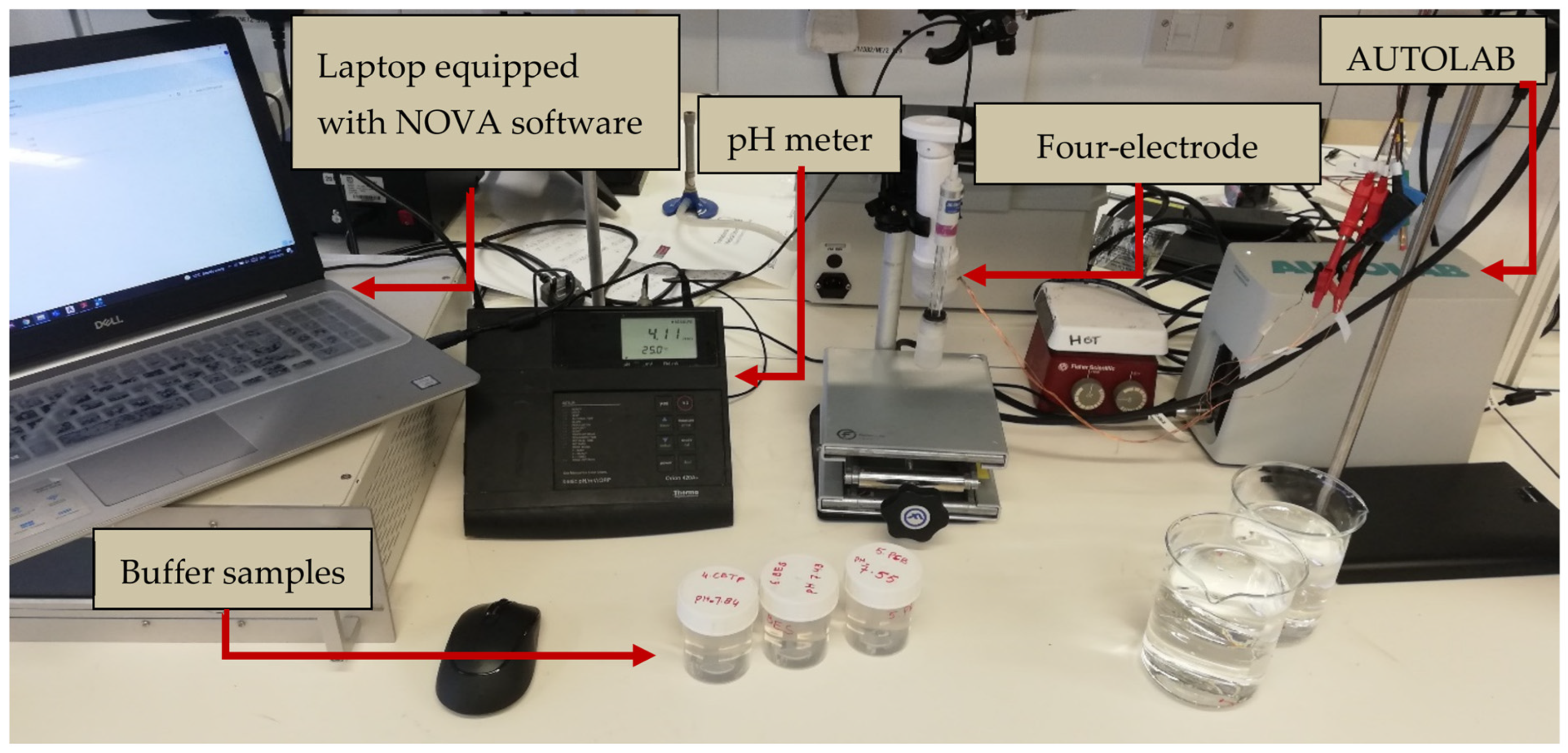
For impedance measurements, the impedance measurement system was set up as displayed in
Figure 3. The measurements were recorded using a PGSTAT204 (Autolab, Kanaalweg Den Haag, The Netherlands), which was set up in galvanostatic mode at room temperature (23 °C). The readings were obtained using a personal computer with Nova 2.1 software and the FRAM32 Impedance Analysis module (Metrohm Autolab B.V., Utrecht, The Netherlands). The measurement setup consisted of the PGSTAT204 connected to a four-point collinear probe, which consisted of a working electrode, counter electrode, reference electrode, and sensing electrode arranged in a collinear pattern [
30]. The galvanostatic mode technique involves the flow of a constant electric current of 100 µA between the inducing electrodes.
The four-electrode collinear probe was fabricated from pure copper with a thickness of 0.5 mm and had electrode diameters of 3 mm and inter-electrode spacings of 2 mm. The probe was characterized, as described in [
31], using saline solutions of concentrations 0.01 M (M = molar = mol/L), 0.05 M, and 0.1 M over the frequency range of 10 Hz to 100 kHz [
32]. The characterization of the impedance probe involves the estimation of the cell constant: The cell constant relates the measured conductance to the corresponding reference conductivity. The cell constant of the collinear probe was calculated using the Pearson correlation coefficient (R) between the measured conductance and reference conductivity of the saline solutions. The cell constant for the proposed collinear probe was determined to be 0.032 m within the frequency range from 10 Hz to 100 kHz.
The accuracy of the probe was assessed using a 0.01 M potassium chloride solution. The accuracy of the probe was evaluated by measuring the impedance within the frequency range of 10 Hz to 100 kHz. The cell constant and the measured conductance were used to calculate the conductivity of the potassium chloride solution [
32]. The probe with the best accuracy with a maximum difference of 10% was selected to record impedance measurements. The results indicated that the designed probe delivered consistent, precise, and reliable impedance measurements.
To collect impedance readings, the frequency sweep was set up at 05 logarithmically spaced steps between 10 Hz and 100 kHz. The conductivity was calculated from the measured frequency-dependent complex impedance data and the cell constant using Equations (6)–(10) [
20]. These equations explain the steps used to calculate conductivity.
where
= impedance in ohms (Ω),
= resistance (Ω), and
X = reactance (Ω).
where
Y = admittance in siemens (S),
G = conductance (S), and
B = susceptance (S).
where
σ is the conductivity of buffer in siemens per meter (S/m) and
k is the cell constant (m).
The temperature and pH of each buffer solution were recorded before the impedance was measured. The impedance measurements were repeated three times, and the mean impedance values were taken to calculate the conductivity for each buffer. Additionally, before taking each measurement, the thermometer, pH electrode, and probe were cleaned with distilled water and dried in the air. The diagram of the measurement system is shown in
Figure 3.
The operating frequency range of 10 Hz to 100 kHz was chosen based on prior research [
32] that utilized impedance spectroscopy to examine blood impedance. Frequencies above 1 MHz have been shown to generate stray capacitances and inductances that can potentially compromise the accuracy of measurements [
33]. According to Buendia et al. [
34], the susceptance at high frequencies is exclusively attributed to parasitic capacitance. Thus, the slope of the graph at high frequencies is equivalent to the level of parasitic capacitance that is present in the experimental setup. For tissue conductivities, parasitic capacitances represent a significant source of systematic error that can result in a reduction in the measured impedance modulus at frequencies greater than 200 kHz [
34].
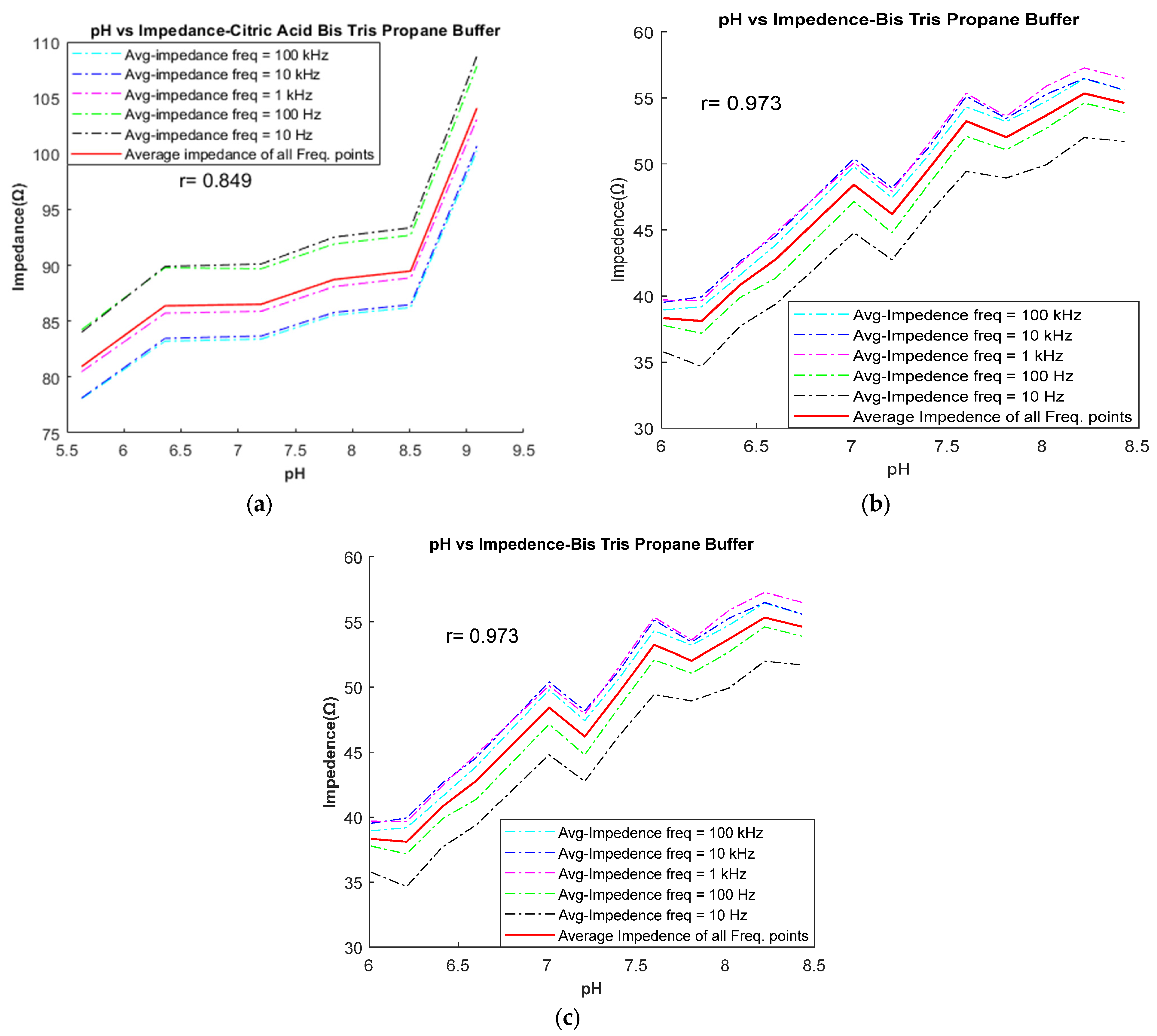
The correlation between the measured pH values and the impedance of each buffer was plotted using MATLAB2020b software.
4. Conclusions and Future Work
In this study, the potential of using ISF pH as a biomarker for hypoxia is considered. The basis for this consideration is two-fold: (1) pH levels quickly change in response to hypoxic events due to the limited buffering capacity of ISF; (2) there is potential to monitor ISF much less invasively compared to blood sampling. To develop novel sensors to monitor ISF pH, there is a requirement to develop electrically representative and pH-representative liquid mimics, and the evaluation of various candidate mimics is described.
In this study, eight buffers were prepared as potential ISF mimics, with pH values ranging from 6.00 to 8.00. All solutions were standardized to a concentration of 0.1 M, and experiments were conducted at room temperature. The candidate buffers were assessed in terms of their pH profile and their electrical conductivity compared to human ISF. Based on our experimental findings, it has been found that the BES buffer and HCl-CBC buffer can effectively mimic the metabolic acidosis induced by asphyxia. Conversely, the metabolic alkalosis effect can be mimicked using BTP, Trizma, and NaOH-BTP.
To the best of the authors’ knowledge, this is the very first study to design ISF-mimicking solutions based on physiological (pH) and electrical properties. As the fabrication of ISF phantoms to evaluate metabolic disorders (or asphyxia) or alkalosis based on electrical characterization is a relatively new approach, there are some limitations to our study. The study primarily focused on mimicking pH and electrical properties and did not directly consider other vital physiological parameters such as oxygen species and carbon dioxide levels. While the effect of these parameters is considered implicitly in terms of pH values, considering these additional parameters in preparing mimicking solutions would provide a more accurate physiological representation of ISF. Another limitation of this study is the lack of measurements of real human ISF for direct comparison of physiological and electrical properties of the interstitial-fluid-mimicking solutions and real human interstitial fluid samples. The practical constraints associated with obtaining sufficient quantities of human interstitial fluid present challenges in conducting these direct comparisons. This limitation restricts the ability to validate the developed interstitial-fluid-mimicking solutions against real ISF samples.
In summary, the current study provides valuable insights into the development of interstitial-fluid-mimicking solutions for hypoxia detection based on pH and electrical properties. However, to enhance the robustness and applicability, future studies can build upon this work by considering additional physiological parameters in preparation of mimicking solutions and incorporating direct comparisons between the prepared interstitial-fluid-mimicking solutions and actual human interstitial fluid samples. These additional analyses would strengthen the evaluation of the interstitial-fluid-mimicking solutions and provide further evidence of their suitability for pre-clinical assessments.


