
An Analytical Study on the Utility of RGB and Multispectral Imagery with Band Selection for Automated Tumor Grading

Abstract
:1. Introduction
2. Materials and Methods
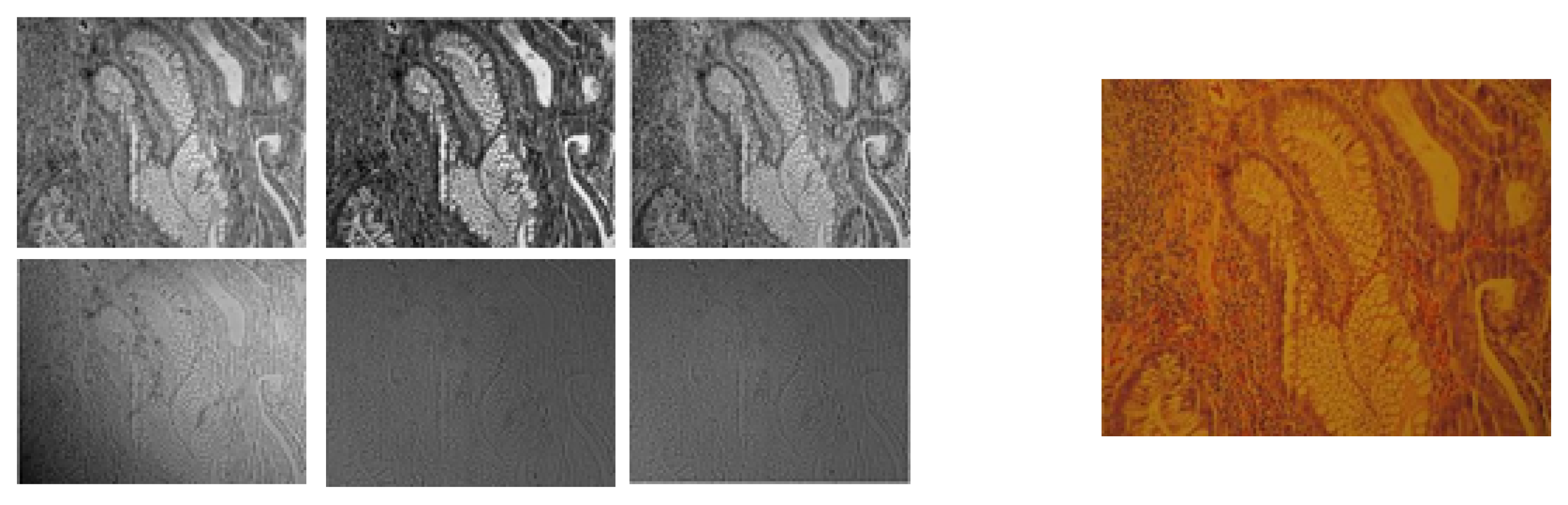
2.1. Image Acquisition
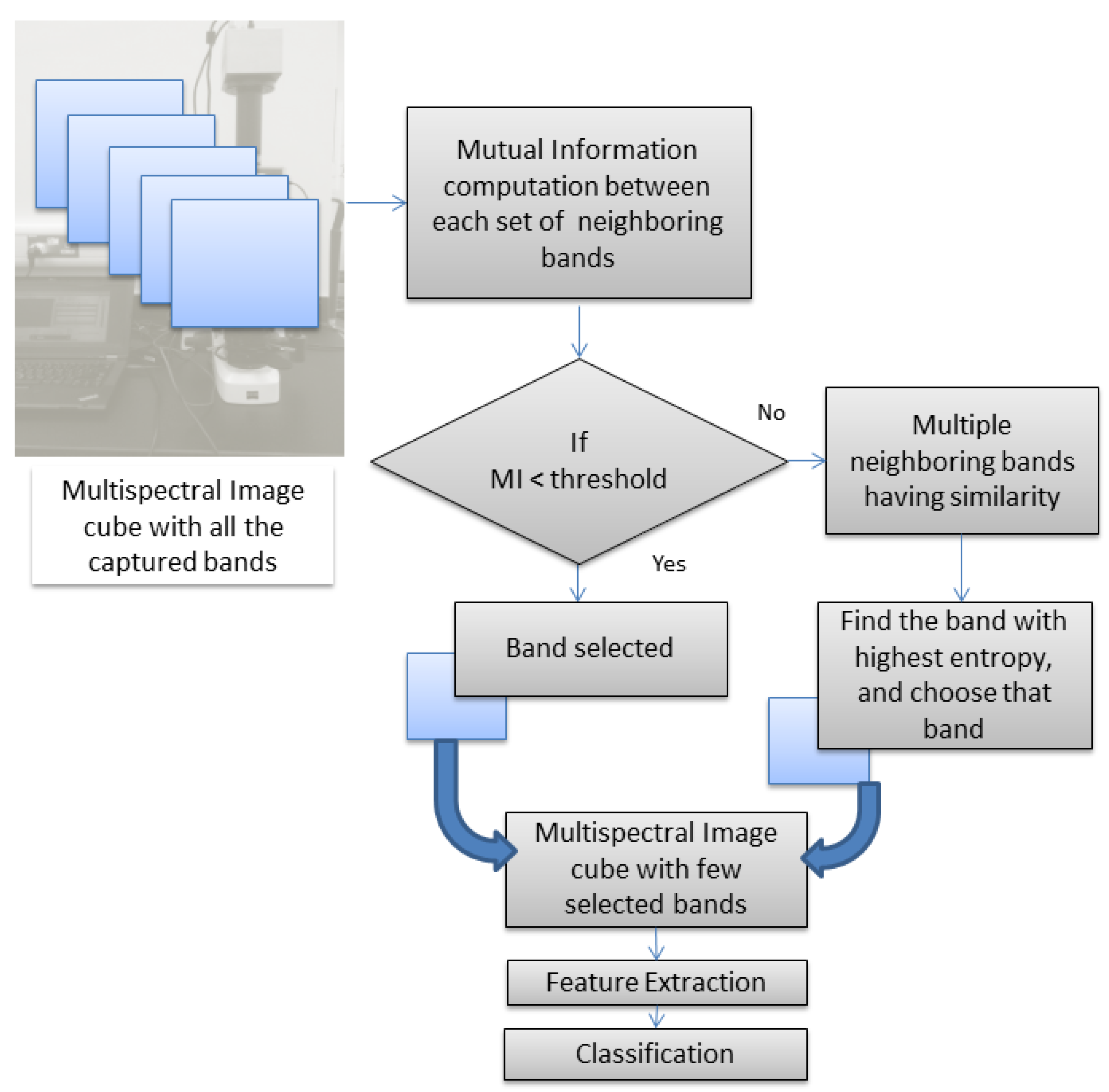
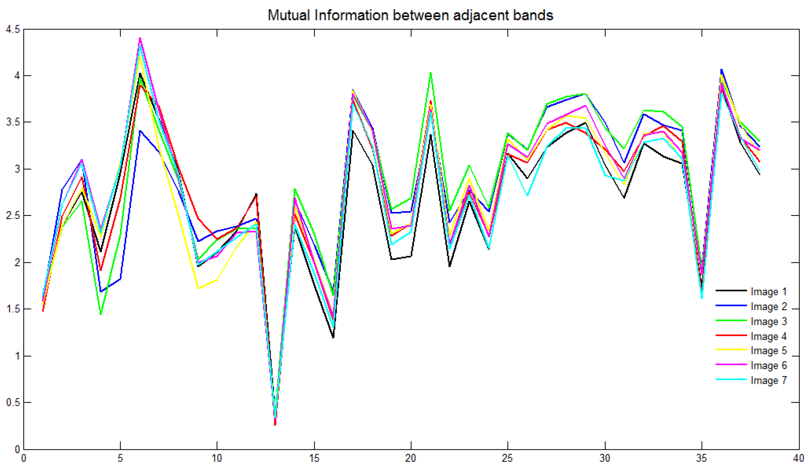
2.2. Band-Selection Method
- is the entropy of random variable A;
- is the entropy of random variable B;
- is the joint entropy of A and B;
- is the conditional entropy of A given B.
2.3. Feature Extraction
2.4. Classification
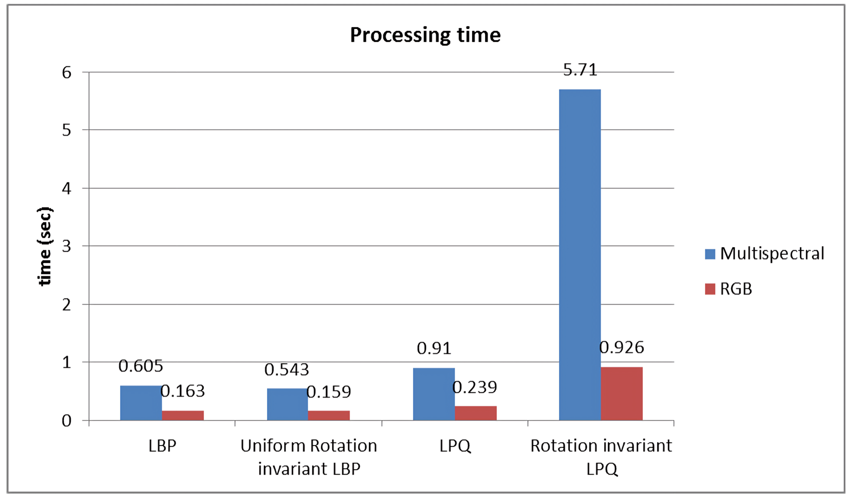
2.5. Performance
3. Results
3.1. RGB vs. Multispectral Imaging
3.2. Band-Selection Approach
4. Discussion
5. Limitations and Future Work
6. Conclusions
Author Contributions
Funding
Institutional Review Board Statement
Informed Consent Statement
Data Availability Statement
Acknowledgments
Conflicts of Interest
References
- Kobayashi, L.C.; von Wagner, C.; Wardle, J. Perceived life expectancy is associated with colorectal cancer screening in England. Ann. Behav. Med. 2017, 51, 327–336. [Google Scholar] [CrossRef] [PubMed]
- Moleyar-Narayana, P.; Leslie, S.; Ranganathan, S. Cancer Screening; StatPearls: Treasure Island, FL, USA, 2024. [Google Scholar]
- Asiedu, M.N.; Guillermo, S.; Ramanujam, N. Low-cost, speculum-free, automated cervical cancer screening: Bringing expert colposcopy assessment to community health. Ann. Glob. Health 2017, 83, 199. [Google Scholar] [CrossRef]
- Cifci, D.; Veldhuizen, G.P.; Foersch, S.; Kather, J.N. AI in computational pathology of cancer: Improving diagnostic workflows and clinical outcomes? Annu. Rev. Cancer Biol. 2023, 7, 57–71. [Google Scholar] [CrossRef]
- Jeleń, Ł.; Fevens, T.; Krzyżak, A. Classification of breast cancer malignancy using cytological images of fine needle aspiration biopsies. Int. J. Appl. Math. Comput. Sci. 2008, 18, 75–83. [Google Scholar] [CrossRef]
- Loukas, C.; Kostopoulos, S.; Tanoglidi, A.; Glotsos, D.; Sfikas, C.; Cavouras, D. Breast cancer characterization based on image classification of tissue sections visualized under low magnification. Comput. Math. Methods Med. 2013, 2013, 829461. [Google Scholar] [CrossRef] [PubMed]
- Araújo, T.; Aresta, G.; Castro, E.; Rouco, J.; Aguiar, P.; Eloy, C.; Polónia, A.; Campilho, A. Classification of breast cancer histology images using Convolutional Neural Networks. PLoS ONE 2017, 12, e0177544. [Google Scholar] [CrossRef] [PubMed]
- Spanhol, F.A.; Oliveira, L.S.; Petitjean, C.; Heutte, L. Breast cancer histopathological image classification using convolutional neural networks. In Proceedings of the 2016 International Joint Conference on Neural Networks (IJCNN), Vancouver, BC, Canada, 24–29 July 2016; IEEE: Piscataway, NJ, USA, 2016; pp. 2560–2567. [Google Scholar]
- Sun, X.; Chuang, S.T.; Li, J.; McKenzie, F. Automatic diagnosis for prostate cancer using run-length matrix method. In Proceedings of the Medical Imaging 2009: Computer-Aided Diagnosis. International Society for Optics and Photonics, Lake Buena Vista, FL, USA, 7–12 February 2009; Volume 7260, pp. 72603H-1–72603H-8. [Google Scholar]
- Alexandratou, E.; Yova, D.; Gorpas, D.; Maragos, P.; Agrogiannis, G.; Kavantzas, N. Texture analysis of tissues in Gleason grading of prostate cancer. In Proceedings of the Imaging, Manipulation, and Analysis of Biomolecules, Cells, and Tissues VI, San Jose, CA, USA, 21–23 January 2008; International Society for Optics and Photonics: Bellingham, WA, USA, 2008; Volume 6859, pp. 685904-1–685904-8. [Google Scholar]
- Ji, H.; Yang, X.; Ling, H.; Xu, Y. Wavelet domain multifractal analysis for static and dynamic texture classification. IEEE Trans. Image Process. 2013, 22, 286–299. [Google Scholar] [CrossRef] [PubMed]
- Lopez, C.; Agaian, S.S. A new set of wavelet-and fractals-based features for Gleason grading of prostate cancer histopathology images. In Proceedings of the Image Processing: Algorithms and Systems XI, Burlingame, CA, USA, 4–6 February 2013; International Society for Optics and Photonics: Bellingham, WA, USA, 2013; Volume 8655, p. 865516. [Google Scholar] [CrossRef]
- Rathore, S.U.R.; Hussain, M.; Iftikhar, M.A.; Jalil, A. Ensemble classification of colon biopsy images based on information rich hybrid features. Comput. Biol. Med. 2014, 47, 76–92. [Google Scholar] [CrossRef] [PubMed]
- Sirinukunwattana, K.; Ahmed Raza, S.E.; Tsang, Y.W.; Snead, D.R.; Cree, I.A.; Rajpoot, N.M. Locality sensitive deep learning for detection and classification of nuclei in routine colon cancer histology images. IEEE Trans. Med. Imaging 2016, 35, 1196–1206. [Google Scholar] [CrossRef]
- Kumar, R.; Srivastava, R.; Srivastava, S. Detection and classification of cancer from microscopic biopsy images using clinically significant and biologically interpretable features. J. Med. Eng. 2015, 2015, 457906. [Google Scholar] [CrossRef]
- Pinckaers, H.; Bulten, W.; van der Laak, J.; Litjens, G. Detection of Prostate Cancer in Whole-Slide Images Through End-to-End Training With Image-Level Labels. IEEE Trans. Med. Imaging 2021, 40, 1817–1826. [Google Scholar] [CrossRef] [PubMed]
- Ström, P.; Kartasalo, K.; Olsson, H.; Solorzano, L.; Delahunt, B.; Berney, D.M.; Bostwick, D.G.; Evans, A.J.; Grignon, D.J.; Humphrey, P.A.; et al. Artificial intelligence for diagnosis and grading of prostate cancer in biopsies: A population-based, diagnostic study. Lancet Oncol. 2020, 21, 222–232. [Google Scholar] [CrossRef] [PubMed]
- Mehta, S.; Lu, X.; Wu, W.; Weaver, D.; Hajishirzi, H.; Elmore, J.G.; Shapiro, L.G. End-to-end diagnosis of breast biopsy images with transformers. Med. Image Anal. 2022, 79, 102466. [Google Scholar] [CrossRef] [PubMed]
- Ikromjanov, K.; Bhattacharjee, S.; Hwang, Y.B.; Sumon, R.I.; Kim, H.C.; Choi, H.K. Whole Slide Image Analysis and Detection of Prostate Cancer using Vision Transformers. In Proceedings of the 2022 International Conference on Artificial Intelligence in Information and Communication (ICAIIC), Jeju Island, Republic of Korea, 21–24 February 2022; pp. 399–402. [Google Scholar] [CrossRef]
- Gao, C.; Sun, Q.; Zhu, W.; Zhang, L.; Zhang, J.; Liu, B.; Zhang, J. Transformer based multiple instance learning for WSI breast cancer classification. Biomed. Signal Process. Control 2024, 89, 105755. [Google Scholar] [CrossRef]
- Wang, K.; Zheng, F.; Cheng, L.; Dai, H.N.; Dou, Q.; Qin, J. Breast Cancer Classification from Digital Pathology Images via Connectivity-aware Graph Transformer. IEEE Trans. Med. Imaging 2024, 1. [Google Scholar] [CrossRef] [PubMed]
- León, R.; Fabelo, H.; Ortega, S.; Cruz-Guerrero, I.A.; Campos-Delgado, D.U.; Szolna, A.; Piñeiro, J.F.; Espino, C.; O’Shanahan, A.J.; Hernandez, M.; et al. Hyperspectral imaging benchmark based on machine learning for intraoperative brain tumor detection. Npj Precis. Oncol. 2023, 7, 119. [Google Scholar] [CrossRef] [PubMed]
- La Salvia, M.; Torti, E.; Leon, R.; Fabelo, H.; Ortega, S.; Balea-Fernandez, F.; Martinez-Vega, B.; Castaño, I.; Almeida, P.; Carretero, G.; et al. Neural networks-based on-site dermatologic diagnosis through hyperspectral epidermal images. Sensors 2022, 22, 7139. [Google Scholar] [CrossRef] [PubMed]
- Petracchi, B.; Gazzoni, M.; Torti, E.; Marenzi, E.; Leporati, F. Machine learning-based classification of skin cancer hyperspectral images. Procedia Comput. Sci. 2023, 225, 2856–2865. [Google Scholar] [CrossRef]
- Petracchi, B.; Torti, E.; Marenzi, E.; Leporati, F. Acceleration of hyperspectral skin cancer image classification through parallel machine-learning methods. Sensors 2024, 24, 1399. [Google Scholar] [CrossRef]
- Al-Maadeed, S.; Kunhoth, S.; Bouridane, A.; Peyret, R. Multispectral imaging and machine learning for automated cancer diagnosis. In Proceedings of the 2017 IEEE 13th International Conference on Wireless Communications and Mobile Computing (IWCMC), Valencia, Spain, 26–30 June 2017; IEEE: Piscataway, NJ, USA, 2017; pp. 1740–1744. [Google Scholar]
- Ortega, S.; Halicek, M.; Fabelo, H.; Callico, G.M.; Fei, B. Hyperspectral and multispectral imaging in digital and computational pathology: A systematic review [Invited]. Biomed. Opt. Express 2020, 11, 3195–3233. [Google Scholar] [CrossRef]
- Kunhoth, S.; Al-Maadeed, S. Building a multispectral image dataset for colorectal tumor biopsy. In Proceedings of the 2017 IEEE 13th International Conference on Wireless Communications and Mobile Computing (IWCMC), Valencia, Spain, 26–30 June 2017; IEEE: Piscataway, NJ, USA, 2017; pp. 1745–1750. [Google Scholar]
- Maes, F.; Collignon, A.; Vandermeulen, D.; Marchal, G.; Suetens, P. Multimodality image registration by maximization of mutual information. IEEE Trans. Med. Imaging 1997, 16, 187–198. [Google Scholar] [CrossRef] [PubMed]
- Ojala, T.; Pietikäinen, M.; Harwood, D. A comparative study of texture measures with classification based on featured distributions. Pattern Recognit. 1996, 29, 51–59. [Google Scholar] [CrossRef]
- Ojala, T.; Pietikäinen, M.; Mäenpää, T. Multiresolution gray-scale and rotation invariant texture classification with local binary patterns. IEEE Trans. Pattern Anal. Mach. Intell. 2002, 24, 971–987. [Google Scholar] [CrossRef]
- Ojansivu, V.; Heikkilä, J. Blur insensitive texture classification using local phase quantization. In Proceedings of the International Conference on Image and Signal Processing, Octeville, France, 1–3 July 2008; Springer: Berlin/Heidelberg, Germany, 2008; pp. 236–243. [Google Scholar]
- Ojansivu, V.; Rahtu, E.; Heikkilä, J. Rotation invariant local phase quantization for blur insensitive texture analysis. In Proceedings of the 2008 19th International Conference on Pattern Recognition, Tampa, FL, USA, 8–11 December 2008; IEEE: Piscataway, NJ, USA, 2008; pp. 1–4. [Google Scholar]
- Schölkopf, B.; Smola, A.J. Learning with Kernels: Support Vector Machines, Regularization, Optimization, and Beyond; MIT Press: Cambridge, MA, USA, 2001. [Google Scholar]
- Chang, C.C.; Lin, C.J. LIBSVM: A library for support vector machines. ACM Trans. Intell. Syst. Technol. (TIST) 2011, 2, 27. [Google Scholar] [CrossRef]
- Kunhoth, S.; Al-Maadeed, S. Multispectral biopsy image based colorectal tumor grader. In Proceedings of the Annual Conference on Medical Image Understanding and Analysis, Edinburgh, UK, 11–13 July 2017; Springer: Cham, Switzerland, 2017; pp. 330–341. [Google Scholar] [CrossRef]
- Kuncheva, L.I. Combining Pattern Classifiers: Methods and Algorithms; John Wiley & Sons: Hoboken, NJ, USA, 2014. [Google Scholar]
- Peyret, R.; Bouridane, A.; Al-Maadeed, S.; Kunhoth, S.; Khelifi, F. Texture analysis for colorectal tumor biopsies using multispectral imagery. In Proceedings of the 2015 37th Annual International Conference of the IEEE Engineering in Medicine and Biology Society (EMBC), Milan, Italy, 25–29 August 2015; IEEE: Piscataway, NJ, USA, 2015; pp. 7218–7221. [Google Scholar] [CrossRef]
- Qi, X.; Cukierski, W.; Foran, D.J. A comparative performance study characterizing breast tissue microarrays using standard RGB and multispectral imaging. In Proceedings of the Multimodal Biomedical Imaging V, San Francisco, CA, USA, 23–25 January 2010; SPIE: Bellingham, WA, USA, 2010; Volume 7557, pp. 206–213. [Google Scholar]
- Qi, X.; Xing, F.; Foran, D.J.; Yang, L. Comparative performance analysis of stained histopathology specimens using RGB and multispectral imaging. In Proceedings of the Medical Imaging 2011: Computer-Aided Diagnosis, Lake Buena Vista, FL, USA, 15–17 February 2011; SPIE: Bellingham, WA, USA, 2011; Volume 7963, pp. 947–955. [Google Scholar]
- Liu, W.; Qu, A.; Yuan, J.; Wang, L.; Chen, J.; Zhang, X.; Wang, H.; Han, Z.; Li, Y. Colorectal cancer histopathology image analysis: A comparative study of prognostic values of automatically extracted morphometric nuclear features in multispectral and red-blue-green imagery. Histol. Histopathol. 2024, 18715. [Google Scholar] [CrossRef]
- Ortega, S.; Halicek, M.; Fabelo, H.; Guerra, R.; Lopez, C.; Lejaune, M.; Godtliebsen, F.; Callico, G.M.; Fei, B. Hyperspectral imaging and deep learning for the detection of breast cancer cells in digitized histological images. In Proceedings of the Spie—The International Society for Optical Engineering; NIH Public Access: Milwaukee, WI, USA, 2020; Volume 11320. [Google Scholar]
- Guo, B.; Gunn, S.; Damper, R.; Nelson, J. Adaptive band selection for hyperspectral image fusion using mutual information. In Proceedings of the 2005 7th International Conference on Information Fusion, Philadelphia, PA, USA, 25–28 July 2005; IEEE: Piscataway, NJ, USA, 2005; Volume 8. [Google Scholar]
- Guo, B.; Gunn, S.R.; Damper, R.I.; Nelson, J.D. Band selection for hyperspectral image classification using mutual information. IEEE Geosci. Remote Sens. Lett. 2006, 3, 522–526. [Google Scholar] [CrossRef]
- Wang, B.; Wang, X.; Chen, Z. Spatial entropy based mutual information in hyperspectral band selection for supervised classification. Int. J. Numer. Anal. Model. 2012, 9, 181–192. [Google Scholar]
- Feng, J.; Jiao, L.; Liu, F.; Sun, T.; Zhang, X. Mutual-information-based semi-supervised hyperspectral band selection with high discrimination, high information, and low redundancy. IEEE Trans. Geosci. Remote Sens. 2015, 53, 2956–2969. [Google Scholar] [CrossRef]
- Martínez-Usó, A.; Pla, F.; Sotoca, J.M.; García-Sevilla, P. Clustering-based hyperspectral band selection using information measures. IEEE Trans. Geosci. Remote Sens. 2007, 45, 4158–4171. [Google Scholar] [CrossRef]

| Method | (c, g) for Multispectral Images | (c, g) for RGB Images |
|---|---|---|
| LBP | 8, 0.0625 | 8, 2 |
| Uniform rLBP | 4, 1 | 8, 2 |
| LPQ | 2, 0.0625 | 8, 0.0625 |
| rLPQ | 8, 0.0625 | 8, 0.25 |
| Method | Multispectral Images (320 × 256 × 39) | RGB Images
(320 × 256 × 3) |
|---|---|---|
| LBP | 77.86 | 65.32 |
| Uniform rLBP | 83.61 | 66.99 |
| LPQ | 67.52 | 65.29 |
| rLPQ | 86.05 | 80.71 |
| Filter Size | 3 | 5 | 7 | 9 |
|---|---|---|---|---|
| Rotation-Invariant LPQ | 86.11 | 86.39 | 87.70 | 86.05 |
| No. of Bands 1 | 22 | 19 | 17 | 10 |
|---|---|---|---|---|
| Filter Size | ||||
| 3 | 86.17 | 85.30 | 83.62 | 78.86 |
| 5 | 86.83 | 87.31 | 86.82 | 85.12 |
| 7 | 87.87 | 87.91 | 87.50 | 87.15 |
| 9 | 86.52 | 86.77 | 86.19 | 85.37 |
| Filter Size | 3 | 5 | 7 | 9 |
|---|---|---|---|---|
| Rotation-Invariant LPQ | 92.21 | 91.96 | 91.68 | 90.32 |
| No. of Bands 1 | 22 | 19 | 17 | 10 |
|---|---|---|---|---|
| Filter Size | ||||
| 3 | 92.57 | 93.83 | 93.77 | 90.11 |
| 5 | 91.44 | 94.09 | 93.96 | 92.75 |
| 7 | 91.22 | 92.24 | 92.60 | 92.86 |
| 9 | 90.73 | 92.39 | 92.55 | 91.84 |
Disclaimer/Publisher’s Note: The statements, opinions and data contained in all publications are solely those of the individual author(s) and contributor(s) and not of MDPI and/or the editor(s). MDPI and/or the editor(s) disclaim responsibility for any injury to people or property resulting from any ideas, methods, instructions or products referred to in the content. |
© 2024 by the authors. Licensee MDPI, Basel, Switzerland. This article is an open access article distributed under the terms and conditions of the Creative Commons Attribution (CC BY) license (https://creativecommons.org/licenses/by/4.0/).
Share and Cite
Kunhoth, S.; Al-Maadeed, S. An Analytical Study on the Utility of RGB and Multispectral Imagery with Band Selection for Automated Tumor Grading. Diagnostics 2024, 14, 1625. https://doi.org/10.3390/diagnostics14151625
Kunhoth S, Al-Maadeed S. An Analytical Study on the Utility of RGB and Multispectral Imagery with Band Selection for Automated Tumor Grading. Diagnostics. 2024; 14(15):1625. https://doi.org/10.3390/diagnostics14151625
Chicago/Turabian StyleKunhoth, Suchithra, and Somaya Al-Maadeed. 2024. "An Analytical Study on the Utility of RGB and Multispectral Imagery with Band Selection for Automated Tumor Grading" Diagnostics 14, no. 15: 1625. https://doi.org/10.3390/diagnostics14151625