

Lightweight Advanced Deep Neural Network (DNN) Model for Early-Stage Lung Cancer Detection


Abstract
1. Introduction
Key Contributions of Our Study
- In this research, we propose a lightweight model to overcome noisy regions, such as graininess, tissues [27], and vessels, namely a Ricker Wavelet Iterative Center Weighted Median Filter (RWICWM).
- To reduce false positives in the disease prediction accuracy, Sørensen–Dice Index-based K-means clustering has been suggested.
- To detect varying size nodules in lungs, Light Spectrum Optimizer-based pulmonary nodule detection (WDSI-LSO) has been used.
- To differentiate lung parenchyma from the segmented lung, a sliding window strategy has been suggested.
- To screen patients for future analysis, a risk screening has been made based on solitary nodule detection using PLCOm2012.
- To appropriately classify lung cancer with high accuracy, a semi-supervised and contrastive learning [28]-based Deep Neural Network (SSCL-DNN) has been proposed.
- The proposed algorithm evolved using a hybrid method and was compared to other algorithms, such as MLP, CNNs, and RNNs. Google Deep Mind was the first to use reinforcement learning technology in 2013.
2. Literature Survey
3. Proposed Methodology
3.1. Processing Phase
- Peak Signal-to-Noise Ratio (PSNR)
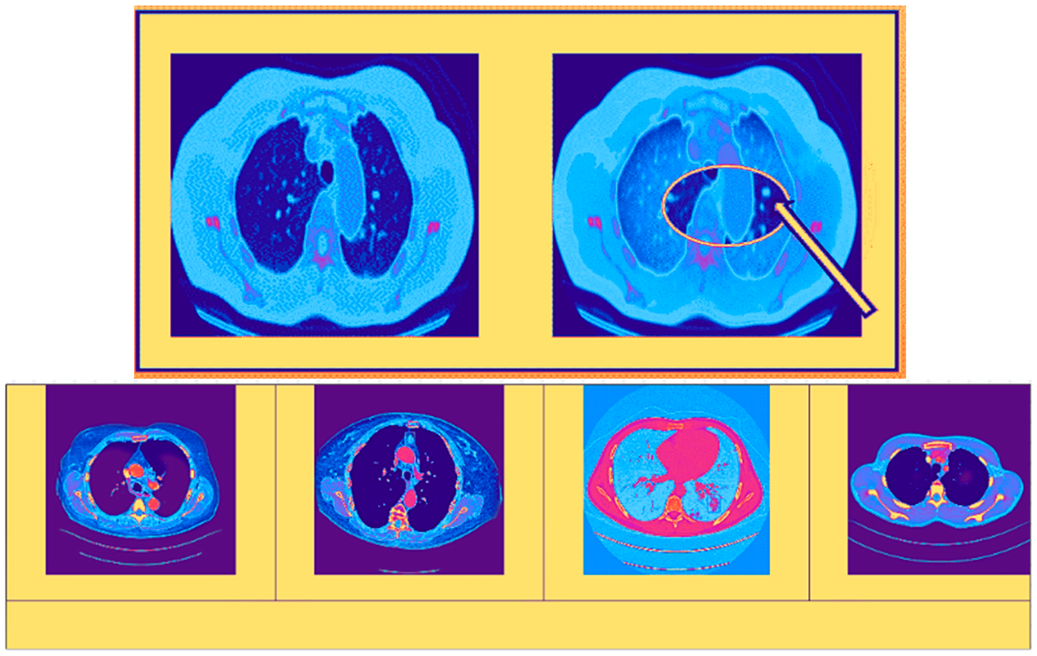
3.2. Segmentation Phase
3.3. Risk Score Screening
3.4. Classification
| Algorithm 1: Proposed Algorithm |
| Input: selected features Output: output categorized as either abnormal or normal Begin Initialize selected features , weight For all training steps do Compute Logistic function Perform convolution layer Perform max pooling layer Process fully connected layer End For Return classified output as Normal or Abnormal End |
3.5. Dataset Description
3.6. Contrastive Learning
4. Results and Discussions
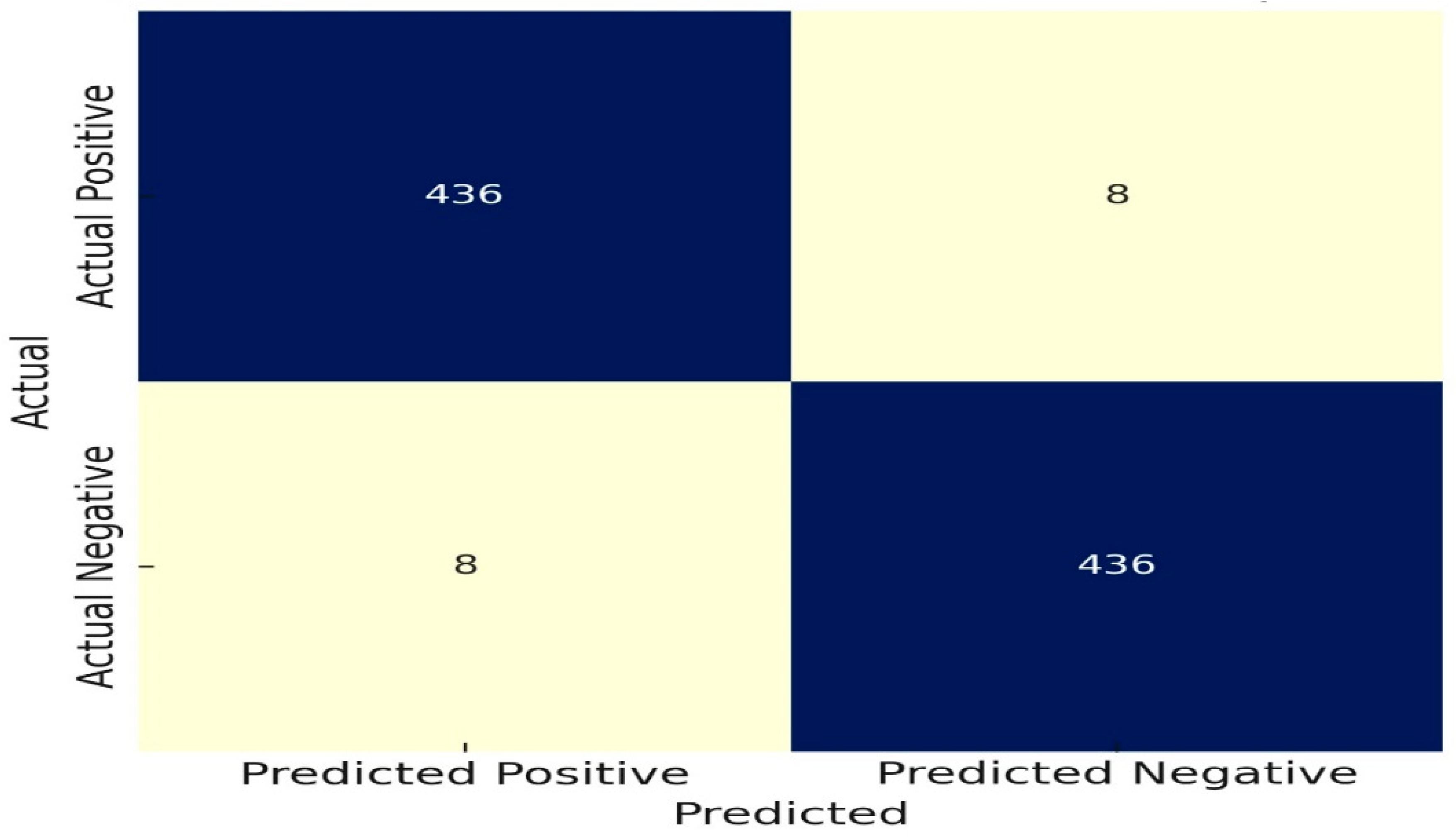
4.1. Experimental Results Using Confusion Matrix
Confusion Matrices
4.2. Evaluating the Lightweight Nature of the Proposed Model
4.2.1. Execution Time
4.2.2. Model Complexity
4.2.3. Resource Usage
4.2.4. High Performance
4.2.5. Comparison of Previous Studies with the Proposed Approach
5. Conclusions
Author Contributions
Funding
Institutional Review Board Statement
Informed Consent Statement
Data Availability Statement
Acknowledgments
Conflicts of Interest
References
- Sun, L.; Zhang, M.; Lu, Y.; Zhu, W.; Yi, Y.; Yan, F. Nodule-CLIP: Lung nodule classification based on multi-modal contrastive learning. Comput. Biol. Med. 2024, 175, 108505. [Google Scholar] [CrossRef] [PubMed]
- Tajidini, F. A comprehensive review of deep learning in lung cancer. arXiv 2023, arXiv:2308.02528. [Google Scholar]
- Kwon, H.-J.; Shin, S.H.; Kim, H.H.; Min, N.Y.; Lim, Y.; Joo, T.-W.; Lee, K.J.; Jeong, M.-S.; Kim, H.; Yun, S.-Y.; et al. Advances in methylation analysis of liquid biopsy in early cancer detection of colorectal and lung cancer. Sci. Rep. 2023, 13, 13502. [Google Scholar] [CrossRef] [PubMed]
- Khodadoust, A.; Nasirizadeh, N.; Seyfati, S.M.; Taheri, R.A.; Ghanei, M.; Bagheri, H. High-performance strategy for the construction of electrochemical biosensor for simultaneous detection of miRNA-141 and miRNA-21 as lung cancer biomarkers. Talanta 2023, 252, 123863. [Google Scholar] [CrossRef]
- Wang, S.; Meng, F.; Li, M.; Bao, H.; Chen, X.; Zhu, M.; Liu, R.; Xu, X.; Yang, S.; Wu, X.; et al. Multidimensional Cell-Free DNA Fragmentomic Assay for Detection of Early-Stage Lung Cancer. Am. J. Respir. Crit. Care Med. 2023, 207, 1203–1213. [Google Scholar] [CrossRef]
- Adams, S.J.; Stone, E.; Baldwin, D.R.; Vliegenthart, R.; Lee, P.; Fintelmann, F.J. Lung cancer screening. Lancet 2023, 401, 390–408. [Google Scholar]
- Sani, S.N.; Zhou, W.; Ismail, B.B.; Zhang, Y.; Chen, Z.; Zhang, B.; Bao, C.; Zhang, H.; Wang, X. LC-MS/MS based volatile organic compound biomarkers analysis for early detection of lung cancer. Cancers 2023, 15, 1186. [Google Scholar] [CrossRef]
- Gunasekaran, K.P. Leveraging object detection for the identification of lung cancer. arXiv 2023, arXiv:2305.15813. [Google Scholar]
- Huang, S.; Yang, J.; Shen, N.; Xu, Q.; Zhao, Q. Artificial intelligence in lung cancer diagnosis and prognosis: Current application and future perspective. In Seminars in Cancer Biology; Academic Press: Cambridge, MA, USA, 2023. [Google Scholar]
- Chabon, J.J.; Hamilton, E.G.; Kurtz, D.M.; Esfahani, M.S.; Moding, E.J.; Stehr, H.; Schroers-Martin, J.; Nabet, B.Y.; Chen, B.; Chaudhuri, A.A.; et al. Integrating genomic features for non-invasive early lung cancer detection. Nature 2020, 580, 245–251. [Google Scholar] [CrossRef]
- Li, W.; Liu, J.-B.; Hou, L.-K.; Yu, F.; Zhang, J.; Wu, W.; Tang, X.-M.; Sun, F.; Lu, H.-M.; Deng, J.; et al. Liquid biopsy in lung cancer: Significance in diagnostics, prediction, and treatment monitoring. Mol. Cancer 2022, 21, 25. [Google Scholar]
- Arulmurugan, R.; Anandakumar, H. Early detection of lung cancer using wavelet feature descriptor and feed forward back propagation neural networks classifier. In Computational Vision and Bio Inspired Computing; Springer International Publishing: Berlin/Heidelberg, Germany, 2018; pp. 103–110. [Google Scholar]
- Gould, M.K.; Donington, J.; Lynch, W.R.; Mazzone, P.J.; Midthun, D.E.; Naidich, D.P.; Wiener, R.S. Evaluation of individuals with pulmonary nodules: When is it lung cancer? Diagnosis and management of lung cancer: American College of Chest Physicians evidence-based clinical practice guidelines. Chest 2013, 143, e93S–e120S. [Google Scholar]
- Pei, Q.; Luo, Y.; Chen, Y.; Li, J.; Xie, D.; Ye, T. Artificial intelligence in clinical applications for lung cancer: Diagnosis, treatment and prognosis. Clin. Chem. Lab. Med. 2022, 60, 1974–1983. [Google Scholar] [CrossRef] [PubMed]
- Chiu, H.-Y.; Chao, H.-S.; Chen, Y.-M. Application of artificial intelligence in lung cancer. Cancers 2022, 14, 1370. [Google Scholar] [CrossRef]
- Mamun, M.; Farjana, A.; Al Mamun, M.; Ahammed, S. Lung cancer prediction model using ensemble learning techniques and a systematic review analysis. In Proceedings of the 2022 IEEE World AI IoT Congress (AIIoT), Seattle, WA, USA, 6–9 June 2022; IEEE: Piscataway, NJ, USA, 2022; pp. 187–193. [Google Scholar]
- Althubiti, S.A.; Paul, S.; Mohanty, R.; Mohanty, S.N.; Alenezi, F.; Polat, K. Ensemble learning framework with GLCM texture extraction for early detection of lung cancer on CT images. Comput. Math. Methods Med. 2022, 2022, 2733965. [Google Scholar] [CrossRef] [PubMed]
- Robbins, H.A.; Alcala, K.; Moez, E.K.; Guida, F.; Thomas, S.; Zahed, H.; Warkentin, M.T.; Smith-Byrne, K.; Brhane, Y.; Muller, D.; et al. Design and methodological considerations for biomarker discovery and validation in the Integrative Analysis of Lung Cancer Etiology and Risk (INTEGRAL) Program. Ann. Epidemiol. 2023, 77, 1–12. [Google Scholar] [CrossRef] [PubMed]
- Fehlmann, T.; Kahraman, M.; Ludwig, N.; Backes, C.; Galata, V.; Keller, V.; Geffers, L.; Mercaldo, N.; Hornung, D.; Weis, T.; et al. Evaluating the use of circulating microRNA profiles for lung cancer detection in symptomatic patients. JAMA Oncol. 2020, 6, 714–723. [Google Scholar] [CrossRef]
- Thakur, S.K.; Singh, D.P.; Choudhary, J. Lung cancer identification: A review on detection and classification. Cancer Metastasis Rev. 2020, 39, 989–998. [Google Scholar] [CrossRef]
- Shahid, F.; Zameer, A.; Muneeb, M. Predictions for COVID-19 with deep learning models of LSTM, GRU and Bi-LSTM. Chaos Solitons Fractals 2020, 140, 110212. [Google Scholar] [CrossRef]
- Oudkerk, M.; Devaraj, A.; Vliegenthart, R.; Henzler, T.; Prosch, H.; Heussel, C.P.; Bastarrika, G.; Sverzellati, N.; Mascalchi, M.; Delorme, S.; et al. Heussel, GorkaBastarrika et al. European position statement on lung cancer screening. Lancet Oncol. 2017, 18, e754–e766. [Google Scholar] [CrossRef]
- Larici, A.R.; Farchione, A.; Franchi, P.; Ciliberto, M.; Cicchetti, G.; Calandriello, L.; del Ciello, A.; Bonomo, L. Lung nodules: Size still matters. Eur. Respir. Rev. 2017, 26, 170025. [Google Scholar] [CrossRef]
- Armato, S.G. Public lung image databases. In Computer-Aided Detection and Diagnosis in Medical Imaging; CRC Press: Boca Raton, FL, USA, 2015; pp. 218–229. [Google Scholar]
- Asuntha, A.; Srinivasan, A. Deep learning for lung Cancer detection and classification. Multimed. Tools Appl. 2020, 79, 7731–7762. [Google Scholar] [CrossRef]
- Kaya, S.I.; Ozcelikay, G.; Mollarasouli, F.; Bakirhan, N.K.; Ozkan, S.A.R. Recent achievements and challenges on nanomaterial based electrochemical biosensors for the detection of colon and lung cancer biomarkers. Sens. Actuators B Chem. 2022, 351, 130856. [Google Scholar] [CrossRef]
- Minegishi, K.; Dobashi, Y.; Koyama, T.; Ishibashi, Y.; Furuya, M.; Tsubochi, H.; Ohmoto, Y.; Yasuda, T.; Nomura, S. Diagnostic utility of trefoil factor families for the early detection of lung cancer and their correlation with tissue expression. Oncol. Lett. 2023, 25, 1–14. [Google Scholar] [CrossRef] [PubMed]
- Sadremomtaz, A.; Zadnorouzi, M. Improving the quality of pulmonary nodules segmentation using the new proposed U-Net neural network. Intell.-Based Med. 2024, 10, 100–166. [Google Scholar]
- Gong, J.; Liu, J.; Li, H.; Zhu, H.; Wang, T.; Hu, T.; Li, M.; Xia, X.; Hu, X.; Peng, W.; et al. Deep learning-based stage-wise risk stratification for early lung adenocarcinoma in CT images: A multi-center study. Cancers 2021, 13, 3300. [Google Scholar] [CrossRef]
- Xia, L.; Mei, J.; Kang, R.; Deng, S.; Chen, Y.; Yang, Y.; Feng, G.; Deng, Y.; Gan, F.; Lin, Y.; et al. Perioperative ctDNA-based molecular residual disease detection for non–small cell lung cancer: A prospective multicenter cohort study (LUNGCA-1). Clin. Cancer Res. 2022, 28, 3308–3317. [Google Scholar] [CrossRef]
- Wang, P.; Huang, Q.; Meng, S.; Mu, T.; Liu, Z.; He, M.; Li, Q.; Zhao, S.; Wang, S.; Qiu, M. Identification of lung cancer breath biomarkers based on perioperative breathomics testing: A prospective observational study. EClinicalMedicine 2022, 47, 101384. [Google Scholar] [CrossRef]
- Isha, B.; Kumar, A. Gait recognition using Hough transform and DWT. Int. J. Adv. Res. Comput. Sci. Softw. Eng. 2014, 4, 889–896. [Google Scholar]
- Vykoukal, J.; Fahrmann, J.F.; Patel, N.; Shimizu, M.; Ostrin, E.J.; Dennison, J.B.; Ivan, C.; Goodman, G.E.; Thornquist, M.D.; Barnett, M.J.; et al. Contributions of circulating microRNAs for early detection of lung cancer. Cancers 2022, 14, 4221. [Google Scholar] [CrossRef]
- Kumar, R.; Saha, P.; Nyarko, R.O.; Lokare, P.; Boateng, A.D.E.; Kahwa, I.; Boateng, P.O.; Asum, C. Effect of COVID-19 in Management of Lung Cancer Disease: A Review. Asian J. Pharm. Res. Dev. 2022, 10, 58–64. [Google Scholar] [CrossRef]
- Huang, H.; Yang, Y.; Zhu, Y.; Chen, H.; Yang, Y.; Zhang, L.; Li, W. Blood protein biomarkers in lung cancer. Cancer Lett. 2022, 551, 215886. [Google Scholar] [CrossRef] [PubMed]
- Salehi, H.; Vahidi, J.; Abdeljawad, T.; Khan, A.; Rad, S.Y.B. A SAR image despeckling method based on an extended adaptive wiener filter and extended guided filter. Remote Sens. 2020, 12, 2371. [Google Scholar] [CrossRef]
- Choi, W.; Oh, J.H.; Riyahi, S.; Liu, C.; Jiang, F.; Chen, W.; White, C.; Rimner, A.; Mechalakos, J.G.; Deasy, J.O.; et al. Radiomics analysis of pulmonary nodules in low-dose CT for early detection of lung cancer. Med. Phys. 2018, 45, 1537–1549. [Google Scholar] [CrossRef] [PubMed]
- Gasparri, R.; Capuano, R.; Guaglio, A.; Caminiti, V.; Canini, F.; Catini, A.; Sedda, G.; Paolesse, R.; Di Natale, C.; Spaggiari, L. Volatolomic urinary profile analysis for diagnosis of the early stage of lung cancer. J. Breath Res. 2022, 16, 046008. [Google Scholar]
- Hackshaw, A.; Clarke, C.A.; Hartman, A.-R. New genomic technologies for multi-cancer early detection: Rethinking the scope of cancer screening. Cancer Cell 2022, 40, 109–113. [Google Scholar] [CrossRef]
- Wang, G.; Qiu, M.; Xing, X.; Zhou, J.; Yao, H.; Li, M.; Yin, R.; Hou, Y.; Li, Y.; Pan, S.; et al. Lung cancer scRNA-seq and lipidomics reveal aberrant lipid metabolism for early-stage diagnosis. Sci. Transl. Med. 2022, 14, eabk2756. [Google Scholar]
- Isha, B.; Aarti, A. Lung carcinoma detection at premature stage using deep learning techniques. In AIP Conference Proceedings; AIP Publishing: Melville, NY, USA, 2022; Volume 2576. [Google Scholar]
- Siegel, R.L.; Miller, K.D.; Fuchs, H.E.; Jemal, A.; Fuchs, B.S.; Ahmedin, J. Cancer statistics, 2022. CA Cancer J. Clin. 2022, 72, 7–33. [Google Scholar] [CrossRef]
- Deb, D.; Moore, A.C.; Roy, U.B. The 2021 global lung cancer therapy landscape. J. Thorac. Oncol. 2022, 17, 931–936. [Google Scholar] [CrossRef]
- Chen, P.; Liu, Y.; Wen, Y.; Zhou, C. Non-small cell lung cancer in China. Cancer Commun. 2022, 42, 937–970. [Google Scholar]
- Gao, Q.; Zeng, Q.; Wang, Z.; Li, C.; Xu, Y.; Cui, P.; Zhu, X.; Lu, H.; Wang, G.; Cai, S.; et al. Circulating cell-free DNA for cancer early detection. Innovation 2022, 3, 100259. [Google Scholar] [CrossRef]
- Hayashi, T.; Kitamura, K.; Hashimoto, S.; Hotomi, M.; Kojima, H.; Kudo, F.; Maruyama, Y.; Sawada, S.; Taiji, H.; Takahashi, G.; et al. Clinical practice guidelines for the diagnosis and management of acute otitis media in children—2018 update. Auris Nasus Larynx 2020, 47, 493–526. [Google Scholar] [PubMed]
- Su, S.; Xuan, Y.; Fan, X.; Bao, H.; Tang, H.; Lv, X.; Ren, W.; Chen, F.; Shao, Y.; Wang, T.; et al. Testing the generalizability of cfDNAfragmentomic features across different studies for cancer early detection. Genomics 2023, 115, 110662. [Google Scholar] [CrossRef] [PubMed]
- Gao, Y.; Chen, Y.; Jiang, Y.; Li, Y.; Zhang, X.; Luo, M.; Wang, X.; Li, Y. Artificial Intelligence Algorithm-Based Feature Extraction of Computed Tomography Images and Analysis of Benign and Malignant Pulmonary Nodules. Comput. Intell. Neurosci. 2022, 2022, 5762623. [Google Scholar] [CrossRef] [PubMed]
- Jayasankari, S.; Domnic, S. Histogram shape based Gaussian sub-histogram specification for contrast enhancement. Intell. Decis. Technol. 2020, 14, 67–80. [Google Scholar] [CrossRef]
- Kim, K.H.; Oh, J.; Yang, G.; Lee, J.; Kim, J.; Gwak, S.-Y.; Cho, I.; Lee, S.H.; Byun, H.K.; Choi, H.-K.; et al. Association of sinoatrial node radiation dose with atrial fibrillation and mortality in patients with lung cancer. JAMA Oncol. 2022, 8, 1624–1634. [Google Scholar] [CrossRef]
- Sharma, A.; Shambhwani, D.; Pandey, S.; Singh, J.; Lalhlenmawia, H.; Kumarasamy, M.; Singh, S.K.; Chellappan, D.K.; Gupta, G.; Prasher, P.; et al. Advances in lung cancer treatment using nanomedicines. ACS Omega 2022, 8, 10–41. [Google Scholar] [CrossRef]
- Kerpel-Fronius, A.; Tammemägi, M.; Cavic, M.; Henschke, C.; Jiang, L.; Kazerooni, E.; Lee, C.-T.; Ventura, L.; Yang, D.; Lam, S.; et al. Screening for lung cancer in individuals who never smoked: An international association for the study of lung cancer early detection and screening committee report. J. Thorac. Oncol. 2022, 17, 56–66. [Google Scholar] [CrossRef] [PubMed]
- Liu, W.; Liu, X.; Li, H.; Li, M.; Zhao, X.; Zhu, Z. Integrating lung parenchyma segmentation and nodule detection with deep multi-task learning. IEEE J. Biomed. Health Inform. 2021, 25, 3073–3081. [Google Scholar] [CrossRef] [PubMed]
- Pradhan, K.; Chawla, P. Medical Internet of things using machine learning algorithms for lung cancer detection. J. Manag. Anal. 2020, 7, 591–623. [Google Scholar] [CrossRef]
- Liu, C.; Xiang, X.; Han, S.; Lim, H.Y.; Li, L.; Zhang, X.; Ma, Z.; Yang, L.; Guo, S.; Soo, R.; et al. Blood-based liquid biopsy: Insights into early detection and clinical management of lung cancer. Cancer Lett. 2022, 524, 91–102. [Google Scholar] [CrossRef]
- Greene, G.; Griffiths, R.; Han, J.; Akbari, A.; Jones, M.; Lyons, J.; Lyons, R.A.; Rolles, M.; Torabi, F.; Warlow, J.; et al. Impact of the SARS-CoV-2 pandemic on female breast, colorectal and non-small cell lung cancer incidence, stage and healthcare pathway to diagnosis during 2020 in Wales, UK, using a national cancer clinical record system. Br. J. Cancer 2022, 127, 558–568. [Google Scholar] [CrossRef] [PubMed]
- Suji, R.J.; Bhadauria, S.S. Automatic Lung Segmentation and Lung Nodule Type Identification over LIDC-IDRI dataset. Indian J. Comput. Sci. Eng. 2021, 12, 1125–1135. [Google Scholar] [CrossRef]
- Niu, C.; Wang, G. Unsupervised contrastive learning based transformer for lung nodule detection. Phys. Med. Biol. 2022, 67, 204001. [Google Scholar] [CrossRef] [PubMed]
- Ren, F.; Xue, S. Intention detection based on siamese neural network with triplet loss. IEEE Access 2020, 8, 82242–82254. [Google Scholar] [CrossRef]


| Stage | Operation | Mathematical Representation |
|---|---|---|
| 1. Input Image | - | (Given Noisy Image) |
| 2. De-noising Filters | Gaussian Filter [49] | |
| Guided Filter [49] | ||
| Wiener Filter [36] | ||
| 3. Histogram Equalization | Histogram Equalization [49] | |
| 4. Quality Metrics | PSNR, MSE, SSIM | |
| Step | Description |
|---|---|
| Input | Medical lung image dataset (labeled and unlabeled). |
| Labeled data indicating the presence/absence of lung cancer. | |
| Pre-trained DNN model for feature extraction. | |
| Output | Segmented lung regions. |
| Predictions of lung cancer likelihood. | |
| Preprocessing | Normalize and preprocess images (resize, crop, intensity normalization). |
| Split the dataset into labeled and unlabeled subsets. | |
| WDSI-LSO Segmentation | Train/Use a pre-trained instance segmentation framework (e.g., Mask R-CNN) on labeled data. Apply the model to unlabeled data to obtain lung region segmentation masks. |
| Train SS-CL-DNN model using features, incorporating semi-supervised techniques. Update the model iteratively using both labeled and unlabeled data. | |
| Contrastive Learning | Implement contrastive learning to enhance feature representations [58]. |
| Use a contrastive loss function (e.g., triplet loss [59] or NT-Xent loss) to learn discriminative features. | |
| Classification and Prediction | Train a classifier on top of learned features. Use the model for classifying new, unlabeled images and generating predictions. |
| Evaluation | Evaluate model performance using appropriate metrics (accuracy, sensitivity, specificity, ROC, AUC) on a validation/test dataset. |
| Post-processing | Apply post-processing techniques to refine segmentation masks or predictions. |
| Deployment | Deploy the trained SS-CL-DNN model in a clinical setting for lung carcinoma identification. |
| Metric | Nodule Detection | Risk Assessment |
|---|---|---|
| Accuracy | 98.20% | 96.80% |
| Recall | 98.20% | 96.80% |
| Precision | 98.20% | 96.80% |
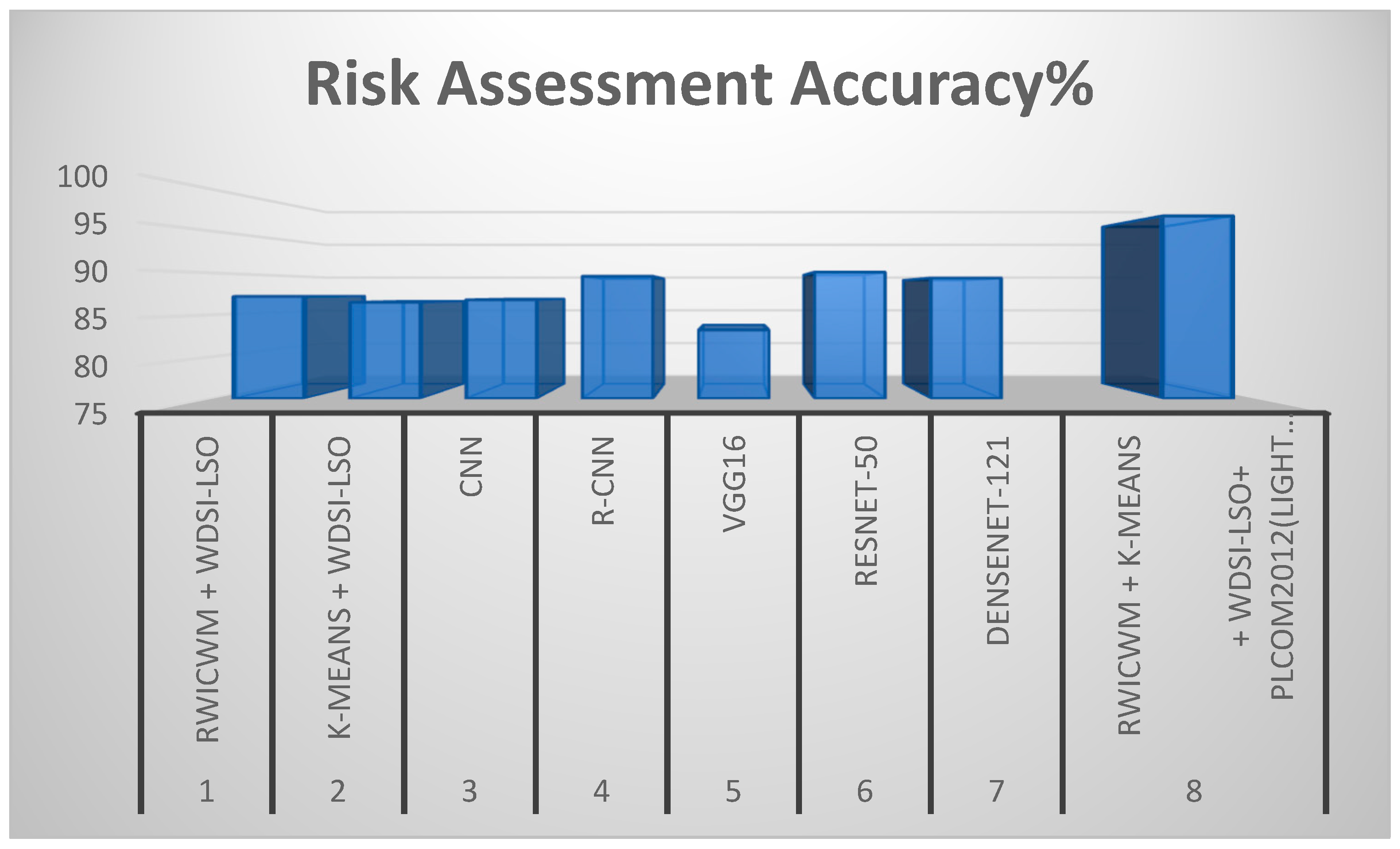
| Experiment | Preprocessing Methods | Nodule Detection Accuracy (%) | Risk Assessment Accuracy (%) |
|---|---|---|---|
| 1 | RWICWM + WDSI-LSO | 95.3 | 87.2 |
| 2 | K-means + WDSI-LSO | 96.1 | 86.5 |
| 3 | CNN | 97.4 | 86.8 |
| 4 | R-CNN | 96.2 | 89.6 |
| 5 | VGG16 | 84.7 | 83.2 |
| 6 | RESNET-50 | 94.5 | 90.1 |
| 7 | DenseNet-121 | 92.8 | 89.4 |
| 8 | RWICWM + K-means + WDSI-LSO + PLCOm2012(Lightweight) | 98.2 | 96.8 |
| Experiment | Preprocessing Method | PSNR | SSIM | Execution Time (s) |
|---|---|---|---|---|
| 1 | RWICWM + WDSI-LSO | 35.2 | 0.89 | 15.3 |
| 2 | K-means + WDSI-LSO | 36.8 | 0.91 | 14.8 |
| 3 | CNN | 37.5 | 0.92 | 18.7 |
| 4 | R-CNN | 36.3 | 0.9 | 20.5 |
| 5 | VGG16 | 34.7 | 0.87 | 22.1 |
| 6 | RESNET-50 | 38.1 | 0.93 | 17.9 |
| 7 | DenseNet-121 | 37 | 0.91 | 16.4 |
| 8 | RWICWM + K-means + WDSI-LSO + PLCOm2012 (Lightweight) | 38.5 | 0.96 | 12.4 |
| Experiment | Model Size (MB) | Inference Time (ms/Image) | Computational Complexity (FLOPs) | Memory Usage (MB) |
|---|---|---|---|---|
| RWICWM + K-means + WDSI-LSO + PLCOm2012 | 45 | 80 | 1.2 × 10⁹ | 250 |
| UNet + WDSI-LSO | 50 | 90 | 1.5 × 10⁹ | 300 |
| InceptionV3 + RWICWM | 70 | 110 | 2.0 × 10⁹ | 350 |
| 3D-CNN + K-means + WDSI-LSO | 65 | 95 | 1.8 × 10⁹ | 320 |
| Hybrid CNN-RNN + RWICWM + PLCOm2012 | 55 | 85 | 1.6 × 10⁹ | 280 |
| Experiment | Preprocessing Methods | Nodule Detection Accuracy (%) | Risk Assessment Accuracy (%) |
|---|---|---|---|
| 1 | RWICWM + K-means + WDSI-LSO + PLCOm2012 (Lightweight) | 98.2 | 96.8 |
| 2 | UNet + WDSI-LSO | 95.9 | 87.9 |
| 3 | InceptionV3 + RWICWM | 96.8 | 88.4 |
| 4 | 3D-CNN + K-means + WDSI-LSO | 97.1 | 89.2 |
| 5 | Hybrid CNN-RNN + RWICWM + PLCOm2012 | 98 | 95.7 |
| Previous Study | Model Architecture | Preprocessing Methods | Nodule Detection Accuracy (%) | Risk Assessment Accuracy (%) | Disadvantages |
|---|---|---|---|---|---|
| Sun et al. (2024) [1] | Nodule-CLIP | Multi-modal contrastive learning | 93.7 | 85.4 | Limited by multi-modal data integration complexity, moderate accuracy. |
| Kwon et al. (2023) [3] | Liquid biopsy analysis | Methylation analysis | 92.3 | 88.0 | High cost and complexity of liquid biopsy, limited to specific biomarkers. |
| Khodadoust et al. (2023) [4] | Electrochemical biosensor | Detection of miRNA biomarkers | 90.5 | 85.2 | Requires specialized equipment, limited to specific biomarkers, moderate accuracy. |
| Wang et al. (2023) [5] | cfDNA Fragmentomic Assay | Cell-free DNA fragment omic assay | 97.0 | 87.3 | High complexity and cost, are not suitable for all clinical settings. |
| Sani et al. (2023) [7] | LC-MS/MS | Volatile organic compound analysis | 91.2 | 84.8 | High cost and complexity, limited to specific biomarkers. |
| Gunasekaran (2023) [8] | Object detection | Object detection algorithms | 89.4 | 82.6 | Lower accuracy compared to more advanced models, less effective for small nodules. |
| Huang et al. (2023) [9] | AI-based diagnostics | AI and machine learning algorithms | 94.6 | 88.7 | High computational requirements, and moderate deployability. |
| Su et al. (2023) [47] | cfDNA fragment omic features | Testing generalizability across studies | 96.5 | 86.2 | Generalizability issues across different datasets, moderate accuracy. |
| Minegishi et al. (2023) [27] | Biomarker analysis | Trefoil factor families | 88.0 | 83.1 | Limited by specific biomarkers, moderate performance. |
| Proposed Model (2024) | Lightweight DNN | RWICWM + K-means + WDSI-LSO + PLCOm2012 | 98.2 | 96.8 | None that are significant, optimally balances speed, accuracy, and efficiency. |
Disclaimer/Publisher’s Note: The statements, opinions and data contained in all publications are solely those of the individual author(s) and contributor(s) and not of MDPI and/or the editor(s). MDPI and/or the editor(s) disclaim responsibility for any injury to people or property resulting from any ideas, methods, instructions or products referred to in the content. |
© 2024 by the authors. Licensee MDPI, Basel, Switzerland. This article is an open access article distributed under the terms and conditions of the Creative Commons Attribution (CC BY) license (https://creativecommons.org/licenses/by/4.0/).
Share and Cite
Bhatia, I.; Aarti; Ansarullah, S.I.; Amin, F.; Alabrah, A. Lightweight Advanced Deep Neural Network (DNN) Model for Early-Stage Lung Cancer Detection. Diagnostics 2024, 14, 2356. https://doi.org/10.3390/diagnostics14212356
Bhatia I, Aarti, Ansarullah SI, Amin F, Alabrah A. Lightweight Advanced Deep Neural Network (DNN) Model for Early-Stage Lung Cancer Detection. Diagnostics. 2024; 14(21):2356. https://doi.org/10.3390/diagnostics14212356
Chicago/Turabian StyleBhatia, Isha, Aarti, Syed Immamul Ansarullah, Farhan Amin, and Amerah Alabrah. 2024. "Lightweight Advanced Deep Neural Network (DNN) Model for Early-Stage Lung Cancer Detection" Diagnostics 14, no. 21: 2356. https://doi.org/10.3390/diagnostics14212356
APA StyleBhatia, I., Aarti, Ansarullah, S. I., Amin, F., & Alabrah, A. (2024). Lightweight Advanced Deep Neural Network (DNN) Model for Early-Stage Lung Cancer Detection. Diagnostics, 14(21), 2356. https://doi.org/10.3390/diagnostics14212356