Bearing Digital Twin Based on Response Model and Reinforcement Learning

Abstract

In recent years, research on bearing fault modeling has witnessed significant advancements. However, the modeling of bearing faults using digital twins (DTs) remains an emerging area of exploration. This paper introduces a bearing digital twin developed by integrating a signal-based response model with reinforcement learning techniques. Initially, a signal-based model is constructed, comprising a unit fault impulse function and a decay oscillation function. This model illustrates the bearing’s acceleration response under fault conditions and acts as the environmental component within the bearing digital twin. Subsequently, a parameter estimation process identifies two critical parameters from the signal-based model: the load proportional factor and the decaying constant. The Deep Deterministic Policy Gradient (DDPG) algorithm is employed as the agent for online learning of these parameters. The cosine similarity metric is employed to define the state and reward by comparing the real acceleration measurements with the simulation data generated by the digital twin. To validate the effectiveness of the digital twin, experimental data sourced from the three datasets are utilized. The results underscore the digital twin’s capacity to faithfully replicate the bearing’s acceleration response under diverse conditions, demonstrating a high degree of similarity in both the time and frequency domains.

1. Introduction

Rolling element bearings serve as critical components within rotating machinery, exerting significant influence over the overall performance of the machine. Modeling techniques are commonly employed to simulate the dynamic behavior of the bearings. Technically, mechanism-based and signal-based methods find extensive application for simulating the vibration response of rolling element bearings under both normal and fault operating conditions [1,2].

The mechanism-based model is formulated through the derivation of force and moment balance equations based on Hertz contact theory. In 1985, S. Fukata introduced an initial dynamic model featuring a two degrees of freedom (2-DoF) configuration, rooted in Hertz contact theory [3]. The research undertaken by the Tiwari group expanded upon this concept, exploring the dynamics of balanced and unbalanced rotors supported by rolling element bearings, thereby characterizing them as nonlinear systems [4,5]. Subsequently, S. Sopanen presented a more comprehensive bearing dynamics model that encompasses the influence of various geometric defects, such as surface roughness, surface waviness, as well as partial and distributed defects, thereby enhancing the fidelity of the bearing model [6,7]. Nevertheless, it is worth noting that the mechanism-based model exhibits certain limitations. This endeavor necessitates a profound understanding of both kinematics and dynamics, resulting in the construction of a notably intricate model. Furthermore, this complexity is compounded by the presence of numerous unmeasured parameters that demand identification. This not only hinders modeling efficiency but also elevates the complexity of real-time parameter identification.

In contrast to the mechanism-based model, the signal-based model boasts a simpler structure and a reduced number of parameters requiring identification. The signal-based modeling places its emphasis on the representation of vibration signals. McFadden and Smith have previously developed a model to describe the high-frequency vibration generated by a single point defect on the inner race under radial load [8], and subsequently extended this model to encompass the vibration produced by multiple point defects [9]. Additionally, Mohammadi introduced a method for detecting multiple defects in bearings based on the time constant within the envelope detector. This technique is employed to discern the characteristic pattern of amplitude variations in defect frequency harmonics within the frequency domain [10]. Various bearing fault characteristics can theoretically be simulated with the same model structure, while the signal-based model exhibits a marginally lower level of accuracy when compared to the mechanism-based model, it compensates with its remarkable modeling efficiency. This heightened efficiency enables the real-time identification of parameters.

As a burgeoning modeling approach, the digital twin possesses the capability to replicate a system using physical information and data gathered from sensors. This capability renders it suitable for application in signal-based modeling. Digital twin applications in bearings have yielded notable outcomes, encompassing three primary avenues: dynamics modeling, fault classification, and remaining useful life prediction. Qin [11] integrated the back-propagation neural network with the digital twin framework to construct a bearing model capable of simulating the life cycle vibration signals. Addressing the challenge of limited data in bearing fault diagnosis, Zhang [12] proposed an innovative digital-twin-driven approach featuring a transformer-based network and a selective adversarial strategy. This approach achieved an 80% accuracy in identifying various types of rolling bearing faults. Xiao [13] introduced a pioneering joint transfer network designed for unsupervised bearing fault diagnosis. This network facilitates knowledge transfer from the simulation domain to the experimental domain. Feng [14] devised an innovative digital-twin-enabled domain adversarial graph network (DTDAGN) that exclusively relies on the structural parameters of bearing dynamics. This novel approach is complemented by a transfer learning framework based on graph convolutional networks. Piltan [15] harnessed machine learning and intelligent digital twins to classify bearing faults and determine crack sizes. Remarkably, accuracy rates of 99.5% and 99.6% were achieved, respectively. Zhang [16] employed the integrated learning CatBoost method to construct a digital twin dataset and utilized fusion features for the life prediction of rolling bearings. Zhao [17] introduced a hybrid approach that combines virtual and real aspects of a bearing digital twin. This approach is based on a modified CycleGAN (generative adversarial network) and Wasserstein distance. It demonstrates the ability to predict the life of rolling bearings with a minimal mean absolute error (MAE) of 0.13.

Updating the model and parameters represents a crucial aspect in the research of digital twin models for diagnosis and prognosis. In the realm of applying digital twin to diagnose faults in rotating machinery, Wang presented a fault diagnosis framework empowered by digital twin technology [18]. In this framework, model updating is conceptualized as an optimization challenge, and it is addressed by employing the particle swarm optimization technique to achieve real-time updates. Aivaliotis [19] employed periodic estimation of modeling parameters utilizing the nonlinear least squares method. Similarly, Xu [20] introduced a novel machine learning technique known as deep transfer learning. This approach exhibits the capability to accurately forecast the evolution of performance during the initial stages of actual manufacturing and to adapt to new working conditions swiftly. Inspired by this intriguing concept, this paper contemplates the utilization of a reinforcement learning algorithm for model updating.

Drawing insights from the aforementioned literature, it becomes apparent that conventional physics-based modeling approaches can leverage intricate mechanisms and structures to establish highly precise models with commendable interpretability and generalizability. Nonetheless, the drawback of these methods lies in their inefficiency due to the requirement of identifying a substantial number of parameters. In contrast, models founded on signal response remedy this inefficiency by adopting a simpler structure and necessitating the identification of fewer parameters. Recognizing this advantage, this study introduces a lightweight bearing digital twin centered around the signal response. The primary objective of this digital twin is to strike a balance between modeling accuracy and efficiency. This is achieved by swiftly identifying a limited number of essential parameters while maintaining interpretability by applying straightforward mechanisms.

• A bearing digital twin is created by fusing a signal-based model with reinforcement learning techniques. The signal-based model is specifically designed to discern and characterize the bearing’s vibration response, encompassing both normal operating conditions and fault scenarios. DDPG is employed to acquire proficiency in learning two crucial parameters integral to the signal-based model. This framework enables the continuous refinement and enhancement of the bearing digital twin by incorporating real-world measurement data.
• The effectiveness of the digital twin is assessed using experimental data obtained from the three datasets. The envelope spectrum error is employed as a metric to compare the acceleration data derived from the physical test bench with that generated by the digital twin. The outcomes of these comparisons unequivocally affirm the viability and soundness of the proposed framework.

The subsequent sections of this paper are organized as follows: Section 2 elucidates the signal-based model devised for capturing bearing vibration responses. In Section 3, the intricate process of bearing digital twin construction is explored, leveraging the signal-based model and incorporating reinforcement learning techniques. Section 4 provides comprehensive insights into the test bench setup and the acquisition of experimental data, which are subsequently used for validation. Section 5 conducts a meticulous analysis of the obtained results. Ultimately, in Section 6, this paper concludes by summarizing the research’s key findings and contributions.

2. Vibration Response Modeling for Bearing with Defects

In this section, a signal-based model will be constructed to analyze bearing responses under fault conditions, serving as the basis of the bearing digital twin. Broadly, the signal-based model integrates various functions to depict the acceleration response characteristics and dynamics of the bearing. These functions encompass load distribution, fault impulse decay, defect-induced vibration, defect localization, and defect width. Subsequently, the modeling theory and process will be introduced in the following sections.

2.1. Modeling for Load Distribution

The load directly determines the bearing’s vibration response. According to Stribeck, the load around the circumference of a rolling element bearing under radial load can be defined as [21]:

$$Q\left(\psi \right)=a·Q_{max}{[1-\frac{1}{2ϵ}(1-cos\psi )]}^n,$$

(1)

where a is the load proportional factor, $Q_{max}$ is the maximum load intensity, $ϵ$ is the load distribution factor, $\psi$ is the angle between the defect and the line of application of load. n is the bearing type factor, with $n=\frac{3}{2}$ for ball bearings and $n=\frac{10}{9}$ for roller bearings.

2.2. Modeling for Fault Impulse Decay

When a bearing exhibits a defect, a sequence of impulses arises as the rolling element traverses the affected area. These impulses undergo continuous oscillation and attenuation owing to the inherent spring and damping characteristics. To capture the vibration response characteristics of the bearing, an approach employing a unit fault impulse function along with a corresponding decay oscillation function is utilized.

2.2.1. Unit Fault Impulse

The assumptions of building unit fault impulse under a certain radial load are as follows. Firstly, it assumes that at $t=0$, the defect is positioned at $\psi =0$, and one of the rolling elements enters into the defect zone, which means an impulse occurs exactly at $t=0$. Secondly, it assumes that the impacts are produced under a unit load distributed uniformly around the bearing. Hence, the vibration produced by the defect can be modeled as an infinite series of impulses with equal amplitude. The unit fault impulse function $d\left(t\right)$ is given by:

$$d\left(t\right)=d_0\sum _{k=-\infty }^{\infty }\delta (t-k{T}_d),$$

(2)

where $\delta \left(t\right)$ stands for the Dirac delta unit impulse function, $d_0$ represents the severity of the defect, and $T_d$ is the time period between the fault impulses. The number of repeated cycles k within one measurement sample can be derived as follows:

$$k=floor\left(\frac{t_s}{\frac{1}{f_d}}\right),$$

(3)

where $t_s$ is the measurement duration of one sample, and $f_d$ represents the defect frequency, which can be substituted by different defect frequencies, such as for the outer race ($f_{\mathrm{BPFO}}$), inner race ($f_{\mathrm{BPFI}}$), cage ($f_{\mathrm{FTF}}$), and ball fault ($f_{\mathrm{BSF}}$).

2.2.2. Decay Oscillation of Fault Impulse

The bearing can be conceptualized as a mass-spring-damping system, where the vibrational impulse resulting from an impact within the defect zone gradually diminishes over time. Hence, the oscillation of the fault impulse can be effectively modeled by the integration of an amplitude function $a\left(t\right)$ and an exponential decay function $e\left(t\right)$. The amplitude function is given by a sinusoidal function, as shown in Equation (4):

$$a\left(\psi \right)=a_0·cos\left(\psi \right)=a_0·cos\left(2\pi f_{n}t\right),$$

(4)

in which $a_0$ represents the actual load applied onto the bearing, and $f_n$ is the bearing system resonance frequency. The exponential function is given by

$$e\left(t\right)=e^{-Bt},$$

(5)

where B is the decaying parameter. This determines the decay rate of the impulse and also represents the bearing fault dynamics. Finally, the decay oscillation $k_d\left(t\right)$ of fault impulse can be defined as the product of an amplitude function $a\left(\psi \right)$ and an exponential decay function $e\left(t\right)$, as follows:

$$k_d\left(t\right)=a\left(\psi \right)\ast e\left(t\right).$$

(6)

2.3. Modeling for Bearing Defect Vibration

By incorporating the effects of bearing load distribution $Q\left(\psi \right)$, unit fault impulse $d\left(t\right)$, and decay oscillation of the fault impulse $a\left(t\right)$ and $e\left(t\right)$, the vibration signal produced by bearing with defects can be reconstructed, as shown in Equation (7):

$$v\left(t\right)=\left[d\right(t)·Q(\psi )·a(\psi \left)\right]\ast e\left(t\right).$$

(7)

Since $\psi$ can be substituted by $2\pi f_{n}t$, the response model can be rewritten, as shown in Equation (8):

$$v\left(t\right)=\left[d\right(t)·q(t)·a(t\left)\right]\ast e\left(t\right),$$

(8)

in which all the parameters can be expressed in the time domain. Besides the general model for vibration signals produced by bearing with defect, this study will also address the modeling of fault position and fault size.

2.4. Modeling for Defect Position

Regarding the modeling of fault positions, it is essential to address distinct scenarios for different bearing components. In the case of the outer ring, typically fixed within the housing, the fault position remains stationary at its initial location, as denoted by Equation (9). Conversely, the inner race, which rotates with the shaft, introduces a variable fault position, as described in Equation (10). Similarly, when a fault occurs on the rolling elements, their positions also change due to their rotation, albeit at different frequencies. This variation is expressed in Equation (11), where $f_r$ represents the shaft rotation frequency, and $f_B$ denotes the revolution frequency of the rolling elements.

$${\psi }_{OR}\left(t\right)={\psi }_{\mathrm{initial}},$$

(9)

$$\hspace{1em}\hspace{1em}\hspace{1em}\hspace{1em}\hspace{1em}\hspace{1em}\hspace{1em}\hspace{1em}{\psi }_{IR}\left(t\right)=({\psi }_{\mathrm{initial}}\left(t\right)+2\pi f_{r}t)mod2\pi ,$$

(10)

$$\hspace{1em}\hspace{1em}\hspace{1em}\hspace{1em}\hspace{1em}\hspace{1em}\hspace{1em}\hspace{1em}{\psi }_B\left(t\right)=({\psi }_{\mathrm{initial}}\left(t\right)+2\pi f_{B}t)mod2\pi .$$

(11)

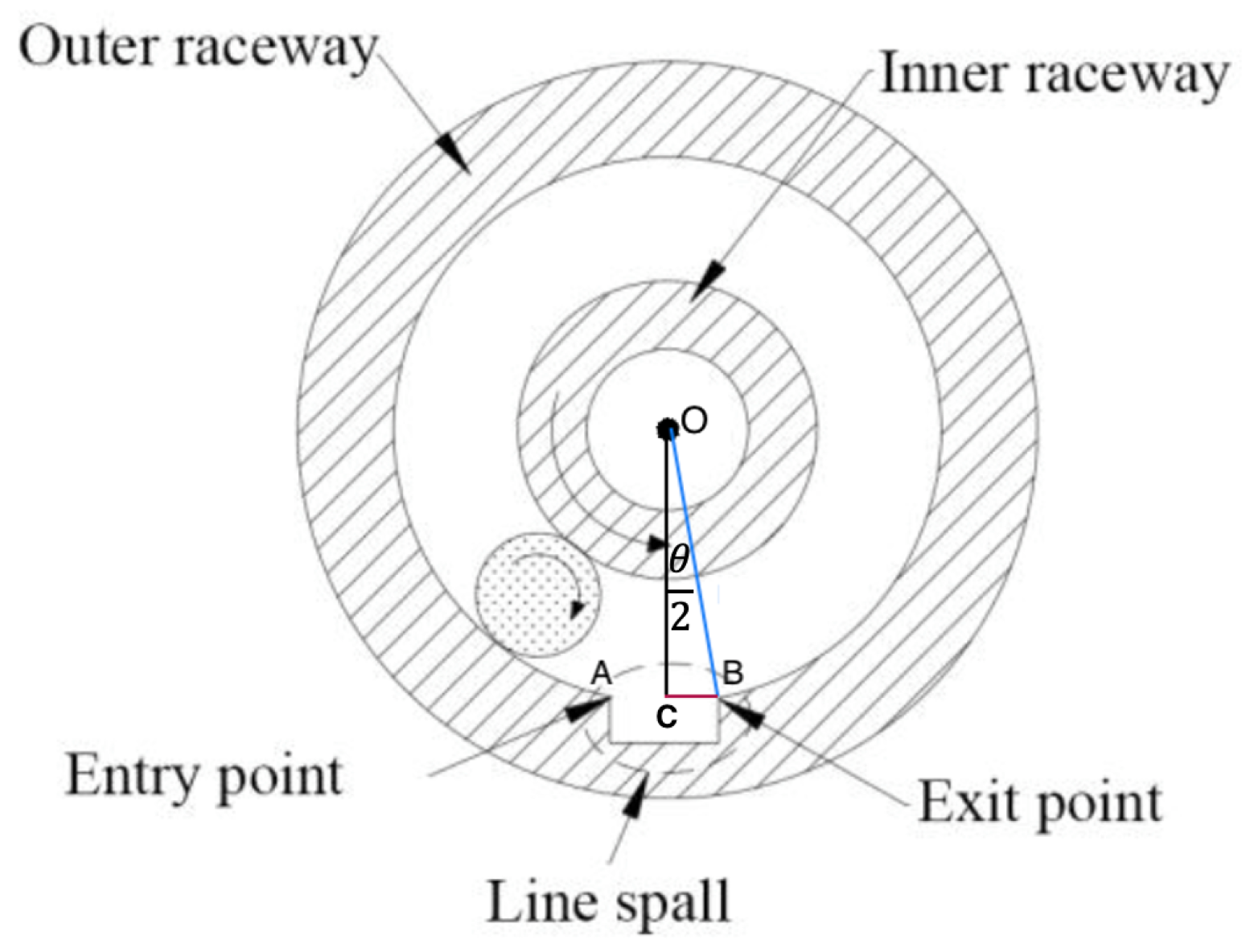
2.5. Modeling for Defect Length

When the ball goes through the entry and exit points, impulses will be generated. As a result, a time lag $\Delta t$ between these two impulses can be observed when the defect length is noticeable. In this subsection, the time lag will be modeled.

As shown in Figure 1, the angle formed by entry point A, the center of ball O, and exit point B are defined as $\theta$. The distance between entry point A and exit point B is the length of the defect and is approximately a straight line when $\theta$ is very small. The angle between $OC$ and $OB$ is $\frac{\theta }{2}$. When the angle is small enough, the relationship between the angle, radius, and the length of defect can be formulated as Equation (12):

$$\theta =sin\left(\theta \right)=2\times \frac{\frac{AB}{2}}{OB}.$$

(12)

Consequently, the period between the rolling balls entering and leaving the defect zone can be calculated as follows:

$$\Delta t=\frac{\theta }{2\pi f_{\mathrm{BPFO}}},$$

(13)

where $f_{\mathrm{BPFO}}$ is the defect frequency of outer race. With the combination of Equations (12) and (13), the time lag of going through the defect can be generally identified as

$$\Delta t=\frac{L}{2\pi f_d\times r},$$

(14)

where L is the defect length, $f_d$ is the defect frequency, and r is the radius. For inner race fault, r can be replaced by $r_{\mathrm{inner}}$ and $f_d$ by $f_{\mathrm{BPFI}}$. Likewise, for ball fault, the r and $f_d$ should be updated with $r_{\mathrm{ball}}$ and $f_{\mathrm{BSF}}$, respectively.

3. Bearing Digital Twin Construction Based on Reinforcement Learning

After establishing the response model of bearing under different fault conditions, the next step is to combine it with reinforcement learning to build a bearing digital twin model.

3.1. Bearing Digital Twin Construction

A digital twin encompasses both physical and virtual domains and delineates the connection or interface between these realms [23]. The behavior of the physical system is subject to alteration based on various factors, including geometrical configurations, material attributes, process variables, operational states, and environmental surroundings. Constructing a digital twin model relies on integrating physical data and sensor measurements, which can be categorized into two core components: physics-based modeling and parameter refinement. The objective of model refinement is to minimize the discrepancy between the dynamic response predicted by the digital twin and the real-time response observed in the physical system.

Figure 2 presents the main procedure for constructing a bearing digital twin. Generally, it includes six steps, as follows:

(1)

The data obtained from the test bench necessitate thorough analysis, and it is imperative to establish the specific conditions under which these data were collected. The condition parameters governing the digital twin, such as the test bearing’s specifications, operational settings, and defect definitions, should align precisely with those employed in the actual test bench.

(2)

The digital twin model will be set up based on the signal-based model. The parameters within this digital twin model can be categorized into two distinct parts: those that are predefined and those that remain unknown. The predefined parameters are derived from the previous step, while the unknown parameters are subject to updates as part of our model updating strategy.

(3)

The data obtained from both the test bench and the digital twin will undergo initial pre-processing. Following this, an envelope spectrum analysis will be performed to establish the foundation for the cost function.

(4)

This cost function will then be computed to quantify the disparity between the data derived from the test bench and those from the digital twin.

(5)

Reinforcement learning will identify the unknown parameters.

(6)

The values of unidentified parameters will be incorporated into the digital twin.

Figure 2. Bearing digital twin structure.

Figure 2. Bearing digital twin structure.

Each episode will go through step (2)–step (6) until the error between the test bench and the digital twin is as small as expected.

3.2. Analysis of Parameters to Be Identified

After introducing the construction of the bearing digital twin, it becomes evident that the updated parameters hold a pivotal role. In this subsection, an analysis will be conducted to determine the parameters requiring updates. The vibration response model generally comprises two primary components: one for load distribution and another for fault impulse decay. The parameters selected for identification will be drawn from these two functions. More specifically, the load proportional factor a plays a critical role in modeling load distribution, defining the range of load distribution around the bearing’s circumference. For a visual representation, please refer to Figure 3, which displays the envelope spectra derived from the vibration response signals under varying load proportional factors.

We can find that the load proportional factor affects the modeling results directly. In the envelope spectrum, the amplitudes at fault peaks will be magnified 100 times when the load proportional factor changes from $a=0.001$ to $a=0.1$. Therefore, the load proportional factor can be selected as a parameter for the digital twin’s online updating. Additionally, the decaying parameter B is crucial for modeling the decay of fault impulse. It affects the decaying rate of the fault impulse. Generally, a large value of B will cause the fault peaks to decay quickly. Otherwise, a small value of B will slow the decaying process. Based on the above analysis, a and B will be selected as the updated parameters in the bearing digital twin model.

3.3. Deep Deterministic Policy Gradient (DDPG)

Once the signal-based model and the relevant parameters have been established, the subsequent crucial step involves devising an appropriate method for parameter identification. In this study, DDPG is employed as the strategy for updating the bearing digital twin model. DDPG is theoretically derived from Policy Gradient (PG) and its extension, Deterministic Policy Gradient (DPG). Unlike DPG, a core enhancement in DDPG is utilizing a convolutional neural network (CNN) instead of the traditional policy structure and value function. Furthermore, these networks are trained using deep learning techniques. For a comprehensive view of the DDPG structure and algorithm, please refer to Figure 4, which illustrates the nine main steps summarized in Algorithm 1.

Algorithm 1 DDPG algorithm

Randomly initialize critic network Q and actor network $\mu$ with weights ${\theta }^Q$ and ${\theta }^{\mu }$. Initialize target network $Q^{\prime }$ and ${\mu }^{\prime }$ with weights ${\theta }^{Q^{\prime }}\leftarrow {\theta }^Q$${\theta }^{{\mu }^{\prime }}\leftarrow {\theta }^{\mu }$. Initialize replay buffer R. for episode = 1: M do     Initialize a random process $\mathcal{N}$ for action exploration.     Receive initial observation state $s_1$.     for t = 1: T do         Select action $a_t=\mu \left(s_t\right|{\theta }^{\mu })+{\mathcal{N}}_t$ according to the current policy and exploration noise.         Execute action $a_t$ and observe reward $r_t$ and observe new state $s_{t+1}$.         Store transition $(s_t,a_t,r_t,s_{t+1})$ in R.         Sample a random mini-batch of N transitions $(s_i,a_i,r_i,s_{i+1})$ from R.         Set target $y_i=r_i+\gamma Q^{\prime }(s_{i+1},{\mu }^{\prime }\left(s_{i+1}\right|{\theta }^{{\mu }^{\prime }})|{\theta }^{Q^{\prime }})$.         Update critic network by minimizing the loss: $L=\frac{1}{N}{\sum }_i{(y_i-Q(s_i,a_i|{\theta }^Q))}^2$.         Update the actor policy network using the sampled gradient:               ${▽}_{{\theta }^{\mu }}\mu |s_i\approx \frac{1}{N}{\sum }_i{▽}_{a}Q(s,a|{\theta }^Q){{|}_{s=s_i,a=\mu \left(s_i\right)}{▽}_{{\theta }^{\mu }}\mu \left(s\right|{\theta }^{\mu })|}_{s_i}$.         Update the target networks:               ${\theta }^{Q^{\prime }}\leftarrow \tau {\theta }^Q+(1-\tau ){\theta }^{Q^{\prime }}$,               ${\theta }^{{\mu }^{\prime }}\leftarrow \tau {\theta }^{\mu }+(1-\tau ){\theta }^{{\mu }^{\prime }}$.     end for end for

3.4. Parameters Identification Based on DDPG

The previous sections introduce the DDPG algorithm and the structure of bearing digital twin. This section will focus on the application of DDPG into digital twin in detail.

3.4.1. Training Environment

The reinforcement learning algorithm has five main elements: agent, environment, state, reward, and action. Their interactions within the DDPG-based bearing digital twin are illustrated in Figure 5.

The agent is the DDPG algorithm, the environment is set up based on bearing digital twin, and the actions are the parameters to be identified: load proportional factor a and decaying parameter B. Both state and reward are defined based on the cost function (C). Specifically, the state is defined as the value of C, while the reward is defined as a piece-wise function of C, as follows:

$$Reward=\{\begin{array}{cc}-100\times C\hfill & C>C_{max},\hfill \\ -10\times C\hfill & C_{min}<C<C_{max},\hfill \\ \frac{10}{C}\hfill & C<C_{min},\hfill \end{array}$$

(15)

where $C_{min}$ and $C_{max}$ are the lower and upper limits of the cost function defined by the user. This particular reward function is defined based on the mechanism. Firstly, segmentation is required, as it allows for quicker convergence in regions with larger errors. Secondly, specific coefficients for each segment are selected using the trial-and-error method. In the following, the construction of the cost function will be introduced.

3.4.2. Cost Function Construction

The construction of the cost function holds particular significance as it directly influences the definitions of state and reward. In this context, the load proportional factor and decaying parameter play a crucial role in shaping the time-domain response of the digital twin. Consequently, the cost function is formulated based on the time domain. To facilitate the training and validation of the digital twin, this study utilizes data spanning a complete fault period. However, before proceeding, the data necessitate pre-processing. The number of data points within one defect period ($L_s$) can be calculated with defect frequency and sampling rate, as follows:

$$L_s=ceil(\frac{1}{f_d}\times f_s),$$

(16)

where $f_d$ is the corresponding defect frequency, $f_s$ is the sampling rate, and $ceil$ stands for the upward rounding function. The maximum value in one defect period has the strongest possibility of being the fault peak. Then, both simulated and test data could be aligned through locating the position of the fault peak. Moreover, only the positive values of the data will be used for cost function calculation.

Regarding the cost function, it is constructed based on cosine similarity, which is a measure of similarity between two non-zero vectors. The cosine similarity is defined as follows:

$$cos\left(\theta \right)=\frac{\overrightarrow{b_{\mathrm{sim}}}·\overrightarrow{b_{\mathrm{real}}}}{\left|\right|\overrightarrow{b_{\mathrm{sim}}}\left|\right|\times \left|\right|\overrightarrow{b_{\mathrm{real}}}\left|\right|},$$

(17)

where $\overrightarrow{b_{\mathrm{sim}}}$ and $\overrightarrow{b_{\mathrm{real}}}$ are two vectors, which will be substituted by simulated data and test data here. $\theta$ is the angle between them. When $\overrightarrow{b_{\mathrm{sim}}}$ and $\overrightarrow{b_{\mathrm{real}}}$ are two vectors with n-dimensions, like $\overrightarrow{b_{\mathrm{sim}}}=[b_{\mathrm{sim},0},b_{\mathrm{sim},1},...,b_{\mathrm{sim},\mathit{n}}]$ and $\overrightarrow{b_{\mathrm{real}}}=[b_{\mathrm{real},0},b_{\mathrm{real},1},...,b_{\mathrm{real},\mathit{n}}]$, the cosine similarity between them should be calculated by every two adjacent points and then averaged over all the cosine similarities. The average value is regarded as the cosine similarity of these n-dimensional vectors. It can be expressed as:

$$cos<\overrightarrow{b_{\mathrm{sim}}},\overrightarrow{b_{\mathrm{real}}}>=\frac{{\displaystyle \sum _{i=1}^n}\frac{(b_{\mathrm{sim},\mathit{i}-1},b_{\mathrm{sim},\mathit{i}})·(b_{\mathrm{real},\mathit{i}-1},b_{\mathrm{real},\mathit{i}})}{\left|\right|(b_{\mathrm{sim},\mathit{i}-1},b_{\mathrm{sim},\mathit{i}})\left|\right|\times \left|\right|(b_{\mathrm{real},\mathit{i}-1},b_{\mathrm{real},\mathit{i}})\left|\right|}}{n},$$

(18)

where vectors $\overrightarrow{b_{\mathrm{sim}}}$ and $\overrightarrow{b_{\mathrm{real}}}$ are simulated data and test data with n-dimensions, respectively. Finally, the cost function based on cosine similarity can be constructed as follows:

$$C=1-cos<\overrightarrow{b_{\mathrm{sim}}},\overrightarrow{b_{\mathrm{real}}}>.$$

(19)

3.4.3. Parameters Setting for DDPG

DDPG algorithm is developed based on the actor–critic method. Both the actor and critic adopt CNN in DDPG. Figure 6 illustrates the structure of the critic and actor networks in bearing digital twin.

The configuration of the critic network is detailed in

Table 1. Parameters of DDPG critic network.

Network Layer	Matlab Network Layer	Number of Inputs
Observation	Feature input layer	1
CriticStateFC1	Fully connected layer	30
CriticRelu1	Relu layer	/
CriticStateFC2	Fully connected layer	30
Action	Feature input layer	2
CriticStateFC2	Fully connected layer	30
Add	Addition Layer	2
CriticCommonRelu	Relu layer	/
CriticOutput	Fully connected layer	1

, while the actor network’s setup is summarized in

Table 2. Parameters of DDPG actor network.

Network Layer	Matlab Network Layer	Number of Inputs
Observation	Feature input layer	1
ActorStateFC1	Fully connected layer	25
ActorRelu1	Relu layer	/
ActorStateFC2	Fully connected layer	2
ActionTanh1	Tanh layer	/
ActorScale1	Scaling layer	/

. Several key parameters deserve attention. Firstly, there is a notable disparity in the learning rates between the actor and critic networks. Typically, the critic network employs a learning rate approximately an order of magnitude larger than that of the actor network. For example, if the critic network’s learning rate is set to 1 $\times {10}^{-3}$, then it is advisable to set the actor network’s learning rate at 1 × 10⁻⁴. This choice is motivated by the fact that the gradient used to update the actor network is derived from the critic network. Secondly, a gradient threshold is introduced as a parameter. Lastly, $L_2$ regularization is employed, introducing a penalty term into the cost function to enhance model robustness, mitigate overfitting, and improve overall accuracy. Specific values for these parameters are provided in

Table 3. Parameters of DDPG neural network.

Parameters	Reference Values
Learning rate of critic network	1 × 10−3
Learning rate of actor network	1 × 10−4
Gradient threshold	1
L2regularization factor	1 × 10−4

. In addition to neural network parameters and regulations, agent settings are also outlined in

Table 4. Parameters of DDPG agent.

Parameters	Reference Values
Experiment buffer length	1 × 10−3
Discount factor	0.99
Mini batch size	128

.

4. Experimental Datasets and Data Processing

After the bearing digital twin has been built, the next step is to validate the model with experiment data. In this section, the test bench used for validation and necessary data pre-processing are introduced.

4.1. Introduction of Bearing Datasets

We employ the Case Western Reserve University (CWRU) dataset as a prime illustration to elucidate the intricate procedures entailed in data processing and meticulous experimental validation [24]. Additionally, to provide further validation of the proposed method’s effectiveness, we conducted comparative experiments employing the Society for Machinery Failure Prevention Technology (MFPT) dataset [25] and the Paderborn University (PU) dataset [26].

Table 5. Bearing specifications of different datasets.

Dataset	CWRU	MFPT	PU
Number of rolling elements	9	8	8
Rolling element diameter (mm)	7.94	0.235	6.75
Pitch diameter (mm)	39.04	1.245	28.55
sample rate (kHz)	12.0	48.8	64.0

summarizes the bearing specifications of these datasets.

As shown in Figure 7, the bearing test bench from CWRU consists of an electric motor, a torque transducer/encoder, a dynamometer, and control electronics. The test bearing connects with the shaft. Table 5 summarizes the bearing specifications. The dataset from the drive end of the motor is collected using accelerometers. There are three bearing defect types: inner race fault, ball fault, and outer race fault. Each bearing fault type has four different fault diameters (0.1778 mm, 0.3556 mm, 0.5334 mm, and 0.7112 mm) and four different motor working loads (745.7 W, 1491.4 W, 2237.1 W, and 2982.8 W).

4.2. Loss Function Based on Envelope Spectrum

Envelope spectrum analysis is an essential tool for bearing diagnostics, from which the unique resonant frequency can be isolated from vibration signals. Thus, the envelope spectrum reveals the repetition frequency of the impulse response series, and the repetition frequency is the bearing fault frequency. The theoretical value of fault frequencies can be calculated as follows, with $f_{\mathrm{BPFO}}$, $f_{\mathrm{BPFI}}$, $f_{\mathrm{FTF}}$, and $f_{\mathrm{BSF}}$ for the outer race, inner race, cage, and ball fault, respectively [27]:

$$\begin{array}{ccc}& & \hfill f_{\mathrm{BPFO}}=\frac{n{f}_r}{2}(1-\frac{d}{D}cos\theta ),\hfill \end{array}$$

(20)

$$\begin{array}{ccc}& & \hfill f_{\mathrm{BPFI}}=\frac{n{f}_r}{2}(1+\frac{d}{D}cos\theta ),\hfill \end{array}$$

(21)

$$\begin{array}{ccc}& & \hfill f_{\mathrm{FTF}}=\frac{f_r}{2}(1-\frac{d}{D}cos\theta ),\hfill \end{array}$$

(22)

$$\begin{array}{ccc}& & \hfill f_{\mathrm{BSF}}=\frac{D{f}_r}{2d}(1-{[\frac{d}{D}cos\theta ]}^2),\hfill \end{array}$$

(23)

where n is the number of rolling elements, $f_r$ is the shaft frequency, $\theta$ is the initial contact angle. d and D are the ball diameter and pitch diameter of a bearing, respectively.

To verify the performance of the digital twin, an essential validation function is defined based on the envelope spectrum. The amplitude and frequency serve as two critical indicators within envelope spectrum analysis after normalization, considering their typical differences in scale [28]. The normalization of amplitudes is subtracting their mean value from the amplitudes of its first five orders and then dividing them by the standard deviation. As given in Equation (24), where $A_{\mathrm{FF}}$ stands for the amplitudes at fault frequencies, as shown with the three red circle positions in Figure 8, $A_{\mu }$ is the mean amplitude of the first five orders, and ${\sigma }_A$ is their standard deviation.

$$A_{\mathrm{FF}}^{\prime }=\frac{A_{\mathrm{FF}}-A_{\mu }}{{\sigma }_A}.$$

(24)

The normalization of frequency is to divide the actual defect frequencies of the first five orders by the theoretical defect frequencies of the fifth order, as formulated in Equation (25):

$$f_i^{\prime }=\frac{f_i}{f_{\mathrm{theo}}\times n_{\mathrm{order}}},$$

(25)

where $f_i$ is the i-th order of actual fault frequency obtained from the envelope spectrum, $f_{\mathrm{theo}}$ represents the first order of theoretical defect frequency, and $n_{\mathrm{order}}$ is the highest order of peak, defined as 5 in this study. After the normalization of amplitudes and frequencies, the deviation between the physical system and the digital twin can be calculated by constructing a validation function:

$$V\left(f\right)=\frac{1}{n}·\sum _{i=1}^n(|A_{\mathrm{real}}^i-A_{\mathrm{sim}}^i{|}^2+|F_{\mathrm{real}}^i-F_{\mathrm{sim}}^i{|}^2),$$

(26)

where $A_{\mathrm{real}}^i$ and $A_{\mathrm{sim}}^i$ represent the amplitude of the i-th order fault peak from the test bench and digital twin, respectively. $F_{\mathrm{real}}^i$ and $F_{\mathrm{sim}}^i$ are the frequency of $i-th$ order fault peak from the test bench and digital twin. This function is employed to evaluate the performance of a digital twin model by quantifying the error in the envelope spectrum when compared to the real measurements obtained from the test bench. The error is determined by comparing the peak information of the digital twin’s simulated data with the test data from the physical system. This error calculation will be refined as the model updates. A digital twin can be considered a suitable substitute for the physical system when the error approaches zero. Conversely, when the error value becomes significantly large, the digital twin model necessitates revision.

5. Results and Analysis

This section presents the training results of the bearing digital twin. The test data consist of measurement samples obtained from the CWRU dataset, encompassing defects on the outer ring, inner ring, and ball components. These data were acquired with a sampling frequency of 12,000 Hz from the drive end under a load of 745.7 W, while the motor operated at a speed of 1772 rpm.

The selected actions consist of the load proportional factor a and the decaying parameter B. The allowable ranges for these two parameters are defined through the output layer of the actor network, specifically set as [0.001, 0.1] and [100, 400], respectively. The training process commences with the dataset sample containing an outer ring defect. At each step, a random value within the same data sample is initiated, and subsequently, the error between the test data and their corresponding simulated data is calculated. Each episode encompasses 80 such steps. The resulting agent undergoes training across 120 episodes and can be effectively applied in diverse environments. To ascertain the agent’s ability to make accurate selections in alternative scenarios, the agent, initially trained on data involving outer ring faults, will be evaluated within environments featuring inner ring and ball defects.

Based on the training results involving states, which represent errors calculated using the cosine similarity cost function, the process entails selecting the smallest state value and subsequently identifying its corresponding action values. These action values are then integrated into the digital twin model.

Table 6. Optimal states in training of DDPG.

Defect Type	Step of Minimum State	Minimum State Value
Outer race	66	0.3203
Inner race	47	0.3130
Ball	23	0.3180

displays the step numbers associated with the minimum states and their corresponding values, which have been acquired through reinforcement learning. Concurrently,

Table 7. Optimal actions identified by DDPG.

Defect Type	Load Proportional Factor a	Decaying Parameter B
Outer race	0.0262	273.5928
Inner race	0.0264	273.0613
Ball	0.0263	272.9066

provides an overview of the corresponding actions. Figure 9 depicts the learning trajectory of the load proportional factor, denoted as ’a,’ and the decaying parameter B. Meanwhile,

Table 8. Validation results based on cosine similarity.

Defect Type	Error from DT	Theoretical Error
Outer race	0.3203	0.2375
Inner race	0.3130	0.2098
Ball	0.3108	0.1123

illustrates the minimum mean error achieved through digital twin training and the calculated mean error resulting from the trained actions. Notably, it is evident that following the identification of the load proportional factor a and decaying parameter B through the DDPG algorithm, the disparity between the simulation data and accurate measurements is greatly reduced.

Upon careful examination of Table 6 and Table 8, it becomes apparent that the errors obtained through digital twin training do not precisely align with the theoretical errors. This discrepancy may be attributed to two key factors. Firstly, an agent trained within a specific environment excels within that environment, resulting in the lowest error percentage when applied to outer ring defect data. Introducing a new environment may potentially impact the performance of the pre-trained agent. Secondly, the initial point of each episode and each step within an episode is characterized by random, unknown values. Consequently, the data employed for comparison and validation differ from those utilized in the DDPG process.

After training, the digital twin model can generate the acceleration response of the bearing under various fault conditions. Figure 10 compares the acceleration data produced by the digital twin and that obtained from the CWRU test bench in both the time and frequency domains. In Figure 10a, “test data” refers to the actual measurement data from the bearing test bench, while “simulated data” signifies the data generated by the digital twin. It is evident that the data generated by the digital twin closely resemble the actual measurement data in terms of overall trends and local features.

Figure 10b compares the frequency domain. Notably, the digital twin accurately captures the fault frequency of the actual measurement sample. However, significant disparities are observed in the time domain of simulated signals. Several factors may contribute to amplitude deviations. Firstly, noise in the actual measurements can influence the envelope spectrum, a factor not addressed in the digital twin model. Secondly, discrepancies in the identification of parameters a and B can lead to variations in response amplitude. Lastly, the simplified signal-based model may not fully represent the intricate dynamics of a real bearing test bench. These same observations and conclusions apply to the acceleration data generated by the digital twin for inner race faults and ball faults.

We conducted ablation experiments using the hyperparameters listed in

Table 9. Hyperparameters used in digital twin as baseline.

Parameter	Mini-Batch Size	Discount Factor	Experience bBuffer Size	Max. Steps
Value	128	0.99	1 × 106	80

as the baseline configuration. The impact of these hyperparameters on the digital twin can be assessed through the experimental outcomes presented in

Table 10. Spectrum error in ablation experiment results.

Hyperparameter		Max.	Min.	Mean	SD
Mini-batch size	32	0.8884	0.5477	0.5633	0.0369
	64	0.5671	0.1082	0.5529	0.0503
	128	0.5996	0.4550	0.5519	0.0158
	256	0.5704	0.2257	0.5538	0.0374
Discount factor	0.93	0.5985	0.3459	0.5904	0.0276
	0.95	0.5984	0.3459	0.5903	0.0276
	0.97	0.8533	0.5552	0.5671	0.0324
	0.99	0.5996	0.4550	0.5519	0.0158
Experience buffer size	1 × 105	0.5704	0.1256	0.5532	0.0484
	1 × 106	0.5996	0.4550	0.5519	0.0158
	1 × 107	0.5669	0.0003	0.5510	0.0622
	1 × 108	0.5765	0.1032	0.5503	0.0325
Max. steps	60	0.5705	0.4832	0.5576	0.0110
	80	0.5996	0.4550	0.5519	0.0158
	100	0.5635	0.2992	0.5553	0.0260
	120	0.5704	0.4459	0.5576	0.0119
Baseline		0.5996	0.4550	0.5519	0.0158

. Among the four parameters, the spectrum error exhibits the highest sensitivity to variations in the discount factor, followed by the mini-batch size. Specifically, their respective average errors reach between 0.5904 and 0.5633, while the average errors observed in other models fall within the range of 0.5503–0.5576.

As the discount factor gradually approaches unity, the standard deviation (SD) of the spectrum error increases, aligning with the trend of error changes associated with the maximum step number. Notably, the samples generated by the baseline model exhibit minimal mean error and relatively low standard deviation compared to the actual samples. This finding substantiates the optimality of the parameters listed in Table 9 for the proposed bearing digital twin.

The MFPT dataset and the PU dataset are used for comparative experiments. The results are shown in

Table 11. Spectrum error in modeling using different datasets.

Dataset	Speed (rpm)	Fault Type	${\mathit{f}}_{\mathit{d}}$ (Hz)	Mean Error	SD	a	B
CWRU	1772	Outer race	105.66	0.5919	0.0158	0.026	274
		Inner race	160.11	1.0304	0.1164	0.026	273
MFPT	1500	Outer race	81.12	0.7616	0.0261	0.014	389
		Inner race	118.88	0.9250	0.1019	0.014	239
PU	900	Outer race	45.81	0.1741	0.0684	0.007	412
		Inner race	74.19	0.1619	0.0743	0.008	618

. In the case of the MFPT dataset, the average error consistently remains below 0.9250. Notably, the SD of the error for the outer race is markedly lower than that for the inner race, a pattern analogous to the findings in the CWRU dataset. When employing the PU dataset, the average error consistently remains below 0.1741, surpassing the performance observed with the CWRU dataset. Moreover, the SD of the errors exhibits a comparable range. These results collectively indicate that the utilization of the PU and MFPT datasets leads to reductions in both the mean and standard deviation of errors. It is reasonable to infer that this improvement can be attributed to the higher sampling frequency, enabling a more faithful representation of the bearing’s true dynamic characteristics. This observation serves to validate the effectiveness of the proposed methodology across diverse bearing datasets.

6. Summary and Conclusions

6.1. Work Summary

Modeling of bearing acceleration response under fault conditions is significant as it provides data to study bearing fault dynamics and can provide data for training fault diagnostics models. This paper proposed a new method to simulate the bearing response by constructing a bearing digital twin. The work finished in this study can be summarized as follows.

• A signal-based model, consisting of a unit impulse function and decay oscillation function, is built to describe the bearing’s acceleration response under different fault conditions, with fault position and length considered.
• A bearing digital twin model is constructed. The signal-based model is taken as the environment, DDPG is adopted as the agent, and the online learning of two parameters (load proportional factor, decaying parameter) from the signal-based model is regarded as the action of the digital twin. In addition, the cosine similarity between the real acceleration and simulation data from the digital twin is utilized to define the reward and state.
• Experimental data from the CWRU test bench are used to validate the proposed bearing digital twin. The acceleration similarity between physics space (test bench) and virtual space (digital twin) in the time and frequency domains is compared.

6.2. Conclusions

Based on the aforementioned work, the following conclusions can be drawn.

• The signal-based model can represent the bearing response under normal and fault conditions. The parameters of the load proportional factor (a) and decaying parameter (B) can be used to identify the fault position and fault dynamics.
• The digital twin can be used to generate the bearing’s acceleration response with high similarity in both time and frequency domains to the real measurement data from the test bench.

6.3. Outlook

The bearing fault modeling is only the basis for a series of follow-up studies in prognostics and health management (PHM). The signal simulated by the bearing digital twin may contain information on the bearing health status and degradation dynamics. Therefore, related further research can include the following directions:

• Exploring the extension of the current signal-based model to characterize defect profiles and accommodate multiple defects is a potential direction for further research.
• Integrating more complex physics models into the digital twin is another area of interest. For instance, combining the Archard model with the signal-based model would enable the modeling of dynamic wear loss and profiles, moving beyond the current focus on static defect size.
• The implementation of the digital twin in an edge system is a topic that merits additional investigation.
• One of the ongoing research directions is the derivation and optimization of hyperparameters in DDPG, which has the potential to improve both modeling accuracy and efficiency significantly.

References

1. Ruan, D.; Chen, Y.; Gühmann, C.; Yan, J.; Li, Z. Dynamics Modeling of Bearing with Defect in Modelica and Application in Direct Transfer Learning from Simulation to Test Bench for Bearing Fault Diagnosis. Electronics 2022, 11, 622. [Google Scholar] [CrossRef]
2. Li, X.; Yu, S.; Lei, Y.; Li, N.; Yang, B. Intelligent Machinery Fault Diagnosis with Event-Based Camera. IEEE Trans. Ind. Inform. 2023. [Google Scholar] [CrossRef]
3. Fukata, S.; Gad, E.H.T. On the Radial Vibration of Ball Bearings. Bull. JSME 1985, 28, 899–904. [Google Scholar] [CrossRef]
4. Tiwari, M.; Gupta, K.; Prakash, O. Effect of radial clearance of a ball bearing on the dynamics of a balanced horizontal rotor. J. Sound Vib. 2000, 238, 723–756. [Google Scholar] [CrossRef]
5. Tiwari, M.; Gupta, K.; Prakash, O. Dynamic response of an unbalanced rotor supported on ball bearing. J. Sound Vib. 2000, 238, 757–779. [Google Scholar] [CrossRef]
6. Sopanen, J.; Mikkola, A. Dynamic model of a deep-groove ball bearing including localized and distributed defects. Part 1: Theory. Proc. Inst. Mech. Eng. 2003, 217, 201–211. [Google Scholar] [CrossRef]
7. Sopanen, J.; Mikkola, A. Dynamic model of a deep-groove ball bearing including localized and distributed defects. Part 2: Implementation and results. Proc. Inst. Mech. Eng. 2003, 217, 213–223. [Google Scholar] [CrossRef]
8. McFadden, P.; Smith, J. Model for the Vibration produced by a Single Point Defect in a Rolling Element Bearing. J. Sound Vib. 1984, 96, 69–82. [Google Scholar] [CrossRef]
9. McFadden, P.; Smith, J. Vibration monitoring of rolling element bearings by the high-frequency resonance technique—A review. Tribol. Int. 1984, 17, 3–10. [Google Scholar] [CrossRef]
10. Mohammadi, A.; Safizadeh, M.S. Bearing Multiple Defects Detection Based on Envelope Detector Time Constant. J. Tribol. 2013, 135, 011102. [Google Scholar] [CrossRef]
11. Qin, Y.; Wu, X.; Luo, J. Data-model combined driven digital twin of life-cycle rolling bearing. IEEE Trans. Ind. Inform. 2021, 18, 1530–1540. [Google Scholar] [CrossRef]
12. Zhang, Y.; Ji, J.; Ren, Z.; Ni, Q.; Gu, F.; Feng, K.; Yu, K.; Ge, J.; Lei, Z.; Liu, Z. Digital twin-driven partial domain adaptation network for intelligent fault diagnosis of rolling bearing. Reliab. Eng. Syst. Saf. 2023, 234, 109186. [Google Scholar] [CrossRef]
13. Xiao, Y.; Shao, H.; Han, S.; Huo, Z.; Wan, J. Novel Joint Transfer Network for Unsupervised Bearing Fault Diagnosis From Simulation Domain to Experimental Domain. IEEE/ASME Trans. Mechatronics 2022, 27, 5254–5263. [Google Scholar] [CrossRef]
14. Feng, K.; Xu, Y.; Wang, Y.; Li, S.; Jiang, Q.; Sun, B.; Zheng, J.; Ni, Q. Digital Twin Enabled Domain Adversarial Graph Networks for Bearing Fault Diagnosis. IEEE Trans. Ind. Cyber-Phys. Syst. 2023, 1, 113–122. [Google Scholar] [CrossRef]
15. Piltan, F.; Kim, J.M. Bearing anomaly recognition using an intelligent digital twin integrated with machine learning. Appl. Sci. 2021, 11, 4602. [Google Scholar] [CrossRef]
16. Zhang, R.; Zeng, Z.; Li, Y.; Liu, J.; Wang, Z. Research on Remaining Useful Life Prediction Method of Rolling Bearing Based on Digital Twin. Entropy 2022, 24, 1578. [Google Scholar] [CrossRef]
17. Zhao, W.; Zhang, C.; Fan, B.; Wang, J.; Gu, F.; Peyrano, O.G.; Wang, S.; Lv, D. Research on rolling bearing virtual-real fusion life prediction with digital twin. Mech. Syst. Signal Process. 2023, 198, 110434. [Google Scholar] [CrossRef]
18. Wang, J.; Ye, L.; Gao, R.X.; Li, C.; Zhang, L. Digital Twin for rotating machinery fault diagnosis in smart manufacturing. Int. J. Prod. Res. 2019, 57, 3920–3934. [Google Scholar] [CrossRef]
19. Aivaliotis, K.P.; Chryssolouris, G. The use of Digital Twin for predictive maintenance in manufacturing. Int. J. Comput. Integr. Manuf. 2019, 32, 1067–1080. [Google Scholar] [CrossRef]
20. Xu, Y.; Sun, Y.; Liu, X.; Zheng, Y. A Digital-Twin-Assisted Fault Diagnosis Using Deep Transfer Learning. IEEE Access 2018, 7, 19990–19999. [Google Scholar] [CrossRef]
21. Harris, T.A.; Kotzalas, M.N. Rolling Bearing Analysis; John Wiley and Sons: New York, NY, USA, 1966. [Google Scholar]
22. Moazenahmad, A.; Dick Petersen, C.H.; Sawalhi, N. Defect size estimation and analysis of the path of rolling elements in defective bearings with respect to the operational speed. In Proceedings of the Inter Noise 2014, Melbourne, Australia, 16–19 November 2019. [Google Scholar]
23. Grieves, M. Virtually Perfect: Driving Innovaitve and Lean Products through Product Lifecycle Management; Space Coast Press: Cocoa Beach, FL, USA, 2011. [Google Scholar]
24. Case Western Reserve University Bearing Data Center Website. Available online: https://csegroups.case.edu/bearingdatacenter/home (accessed on 26 January 2023).
25. Condition Based Maintenance Fault Database for Testing of Diagnostic and Prognostics Algorithms. Available online: https://www.mfpt.org/fault-data-sets/ (accessed on 23 October 2023).
26. Bearing Data Center, KAt-Data Center, Paderborn University. Available online: http://groups.uni-paderborn.de/kat/BearingDataCenter/ (accessed on 23 October 2023).
27. Randall, R.B.; Antoni, J. Rolling element bearing diagnostics—A tutorial. Mech. Syst. Signal Process. 2011, 25, 485–520. [Google Scholar] [CrossRef]
28. Ruan, D.; Song, X.; Gühmann, C.; Yan, J. Collaborative optimization of CNN and GAN for bearing fault diagnosis under unbalanced datasets. Lubricants 2021, 9, 105. [Google Scholar] [CrossRef]
Figure 1. A rolling element traveling into the defect zone located on the outer raceway [22].
Lubricants 11 00502 g001
Figure 3. Envelope spectra under different load factors.
Lubricants 11 00502 g003
Figure 4. Structure of DDPG.
Lubricants 11 00502 g004
Figure 5. Structure of bearing digital twin’s parameters identification based on DDPG.
Lubricants 11 00502 g005
Figure 6. Critic and actor-network structure of DDPG.
Lubricants 11 00502 g006
Figure 7. Bearing test bench from CWRU.
Lubricants 11 00502 g007
Figure 8. Inner race fault defect frequencies of first five orders.
Lubricants 11 00502 g008
Figure 9. Training results of digital twin under different environments.
Lubricants 11 00502 g009
Figure 10. Training results of digital twin (time domain and frequency domain).
Lubricants 11 00502 g010