Effect of Structural Flexibility of Wheelset/Track on Rail Wear


Abstract
:1. Introduction
2. Rail Wear Prediction Model
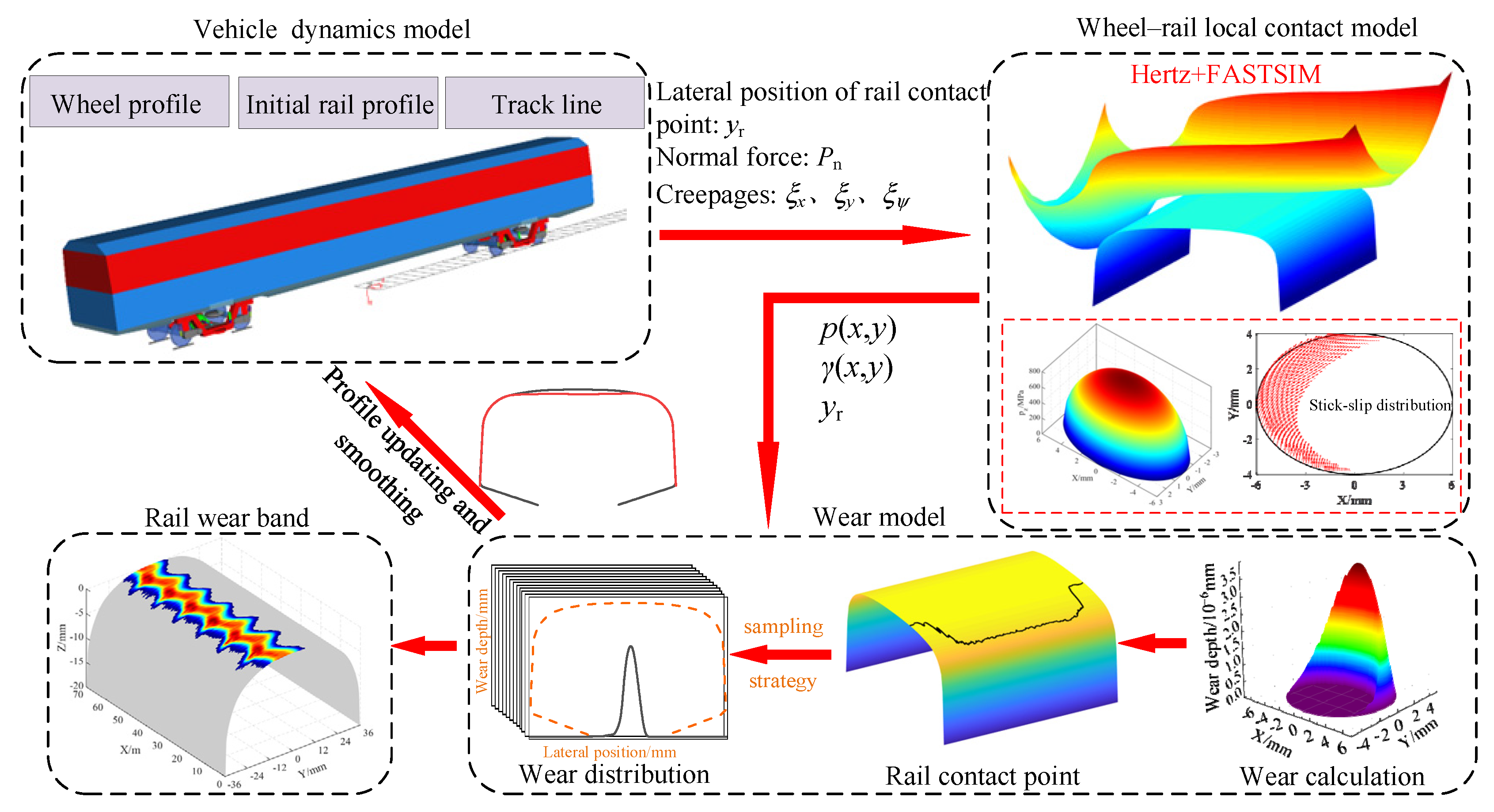
2.1. Three-Dimensional Rail Wear Prediction Process
- (1)
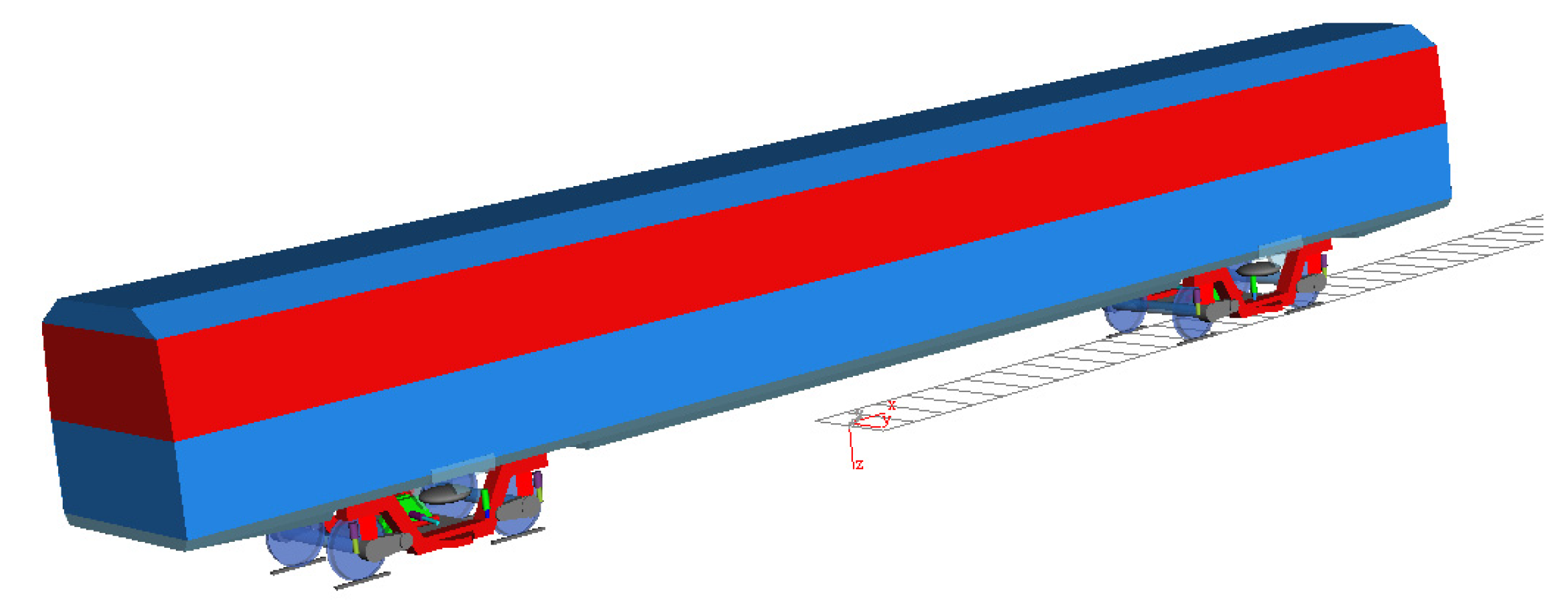
- The vehicle dynamic model is established using the dynamics software SIMPACK. The track parameters and profiles of wheel and rail are set for dynamic simulation. The wheel–rail contact parameters, such as the lateral position of the rail contact point yr, the normal force N, the longitudinal creepage ξx, the lateral creepage ξy, and the spin creepage ξψ, are obtained from output results and used for post-processing.
- (2)
- The contact parameters are used as inputs to the local contact model. The Hertzian theory is used to solve the normal contact to obtain the semi-axes in the rolling direction (a) and lateral direction (b), and the contact pressure distribution. The FASTSIM algorithm [30] is used to obtain the local tangential stress and creep distributions.
- (3)
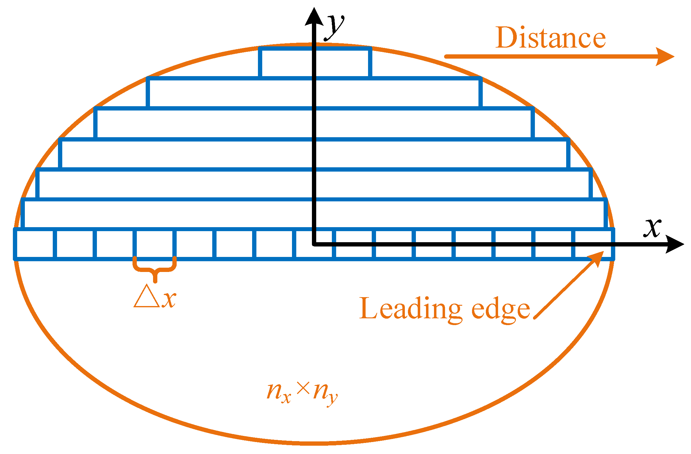
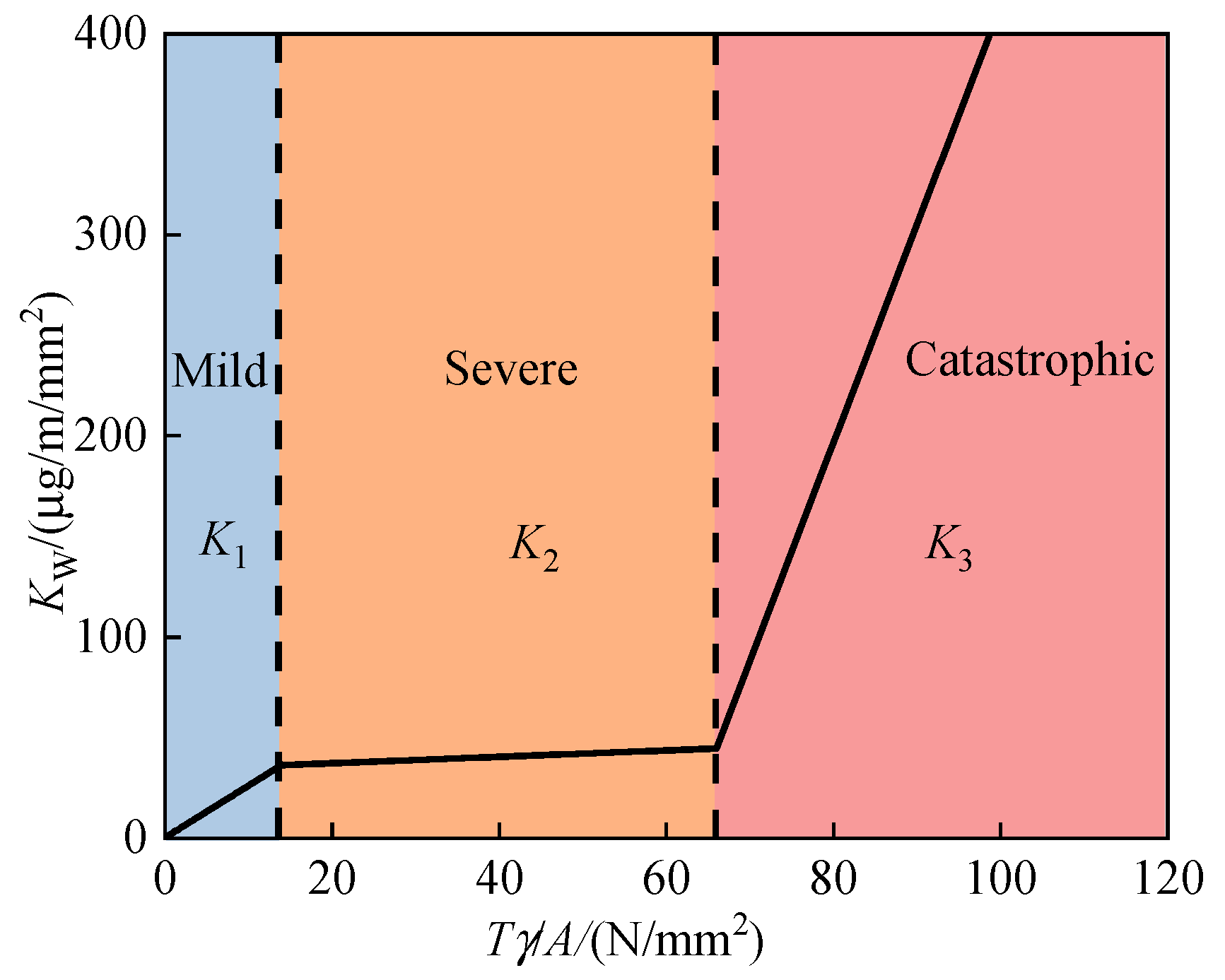
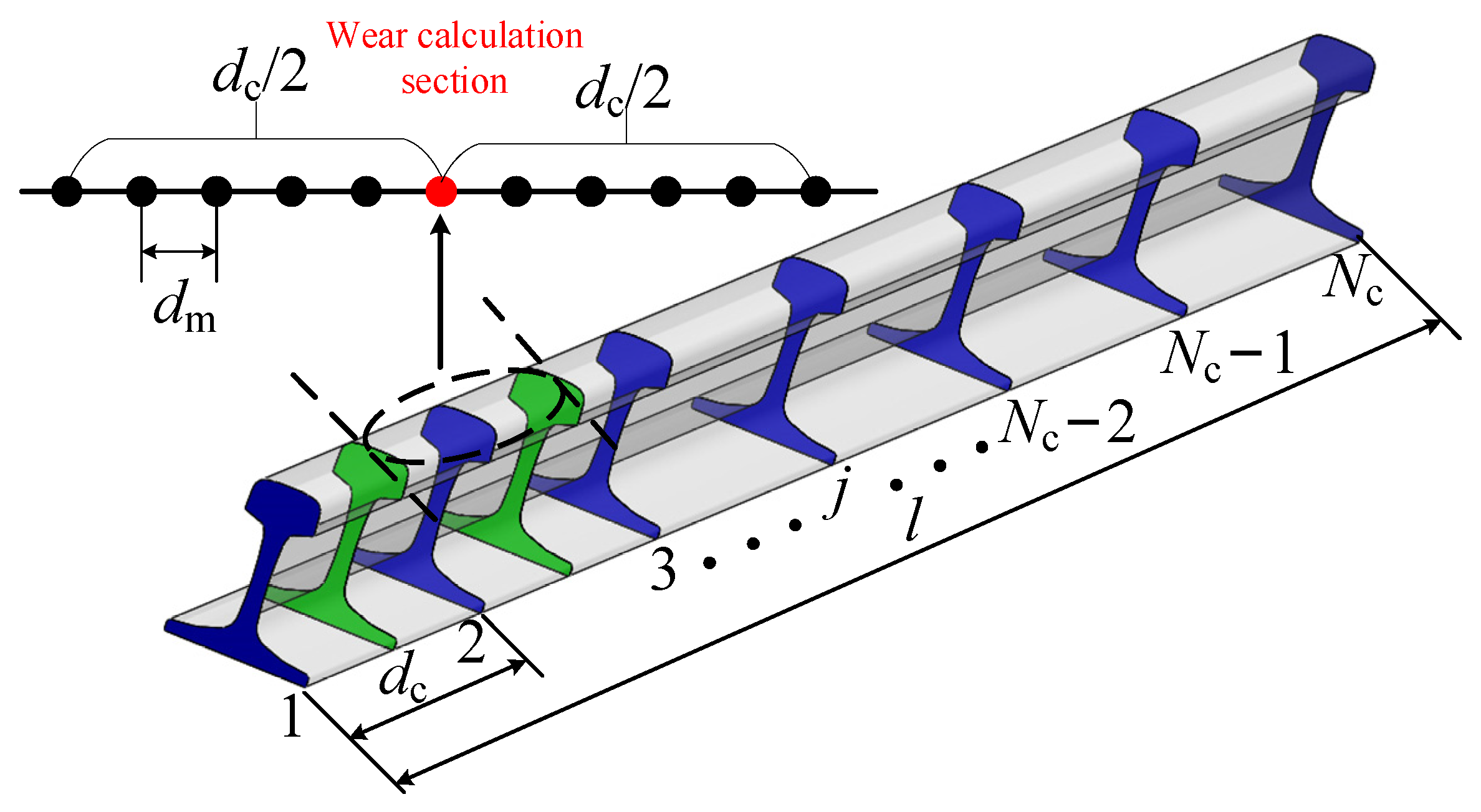
- The results obtained in the previous step are incorporated into the wear model that uses the Tγ/A-wear rate function based on the rail material U75V [31] to estimate the wear distribution at the contact patch. The wear distributions at different cross sections are determined considering the lateral position yr of the rail contact points on the different cross sections and the sampling strategy.
- (4)
- The rail wear distribution generated in this iteration is smoothed using the moving average smoothing method. The wear distributions are scaled up for all cross sections according to the predefined updating strategy. In this step, the rail profiles at different longitudinal positions in the normal direction are removed based on the smoothed rail wear distribution. Then, the rail profile obtained after the removal of wear is smoothed using the cubic spline interpolation smoothing method.
- (5)
- The rail profile after wear removal is imported into the vehicle dynamic model for the next iterative calculation. This process is repeated until the simulation requirements are met.
- (1)
- The evolution of wheel wear is not considered.
- (2)
- The plastic deformation and work hardening during rail wear are not considered.
- (3)
- The influence of vehicle traction and braking on rail wear is ignored.
2.2. Multi-Rigid-Body Dynamic Model
2.3. Wheel–Rail Local Contact Model
2.4. Wear Model
2.5. Sampling and Updating Strategy
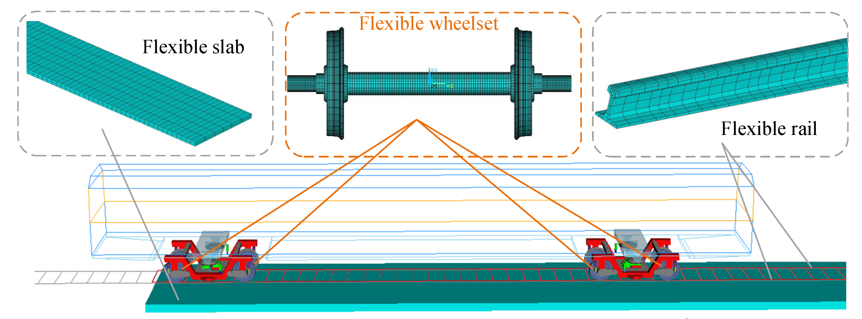
3. Flexibility of Wheelset and Track Structure
3.1. Flexibility of Wheelset
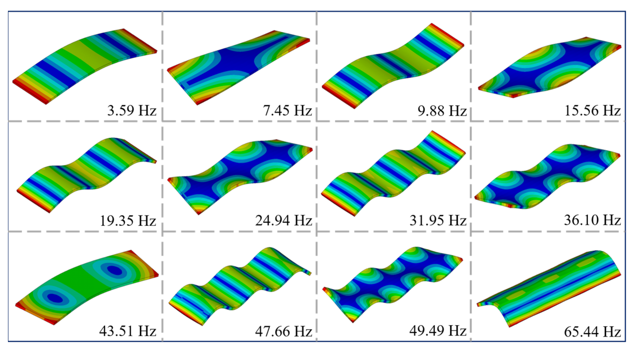
3.2. Flexibility of Track
3.3. Verification of Rigid-Flexible Coupled Dynamic Model
4. Analysis of Simulation Results
4.1. Lateral Position Distribution of Rail Contact Point
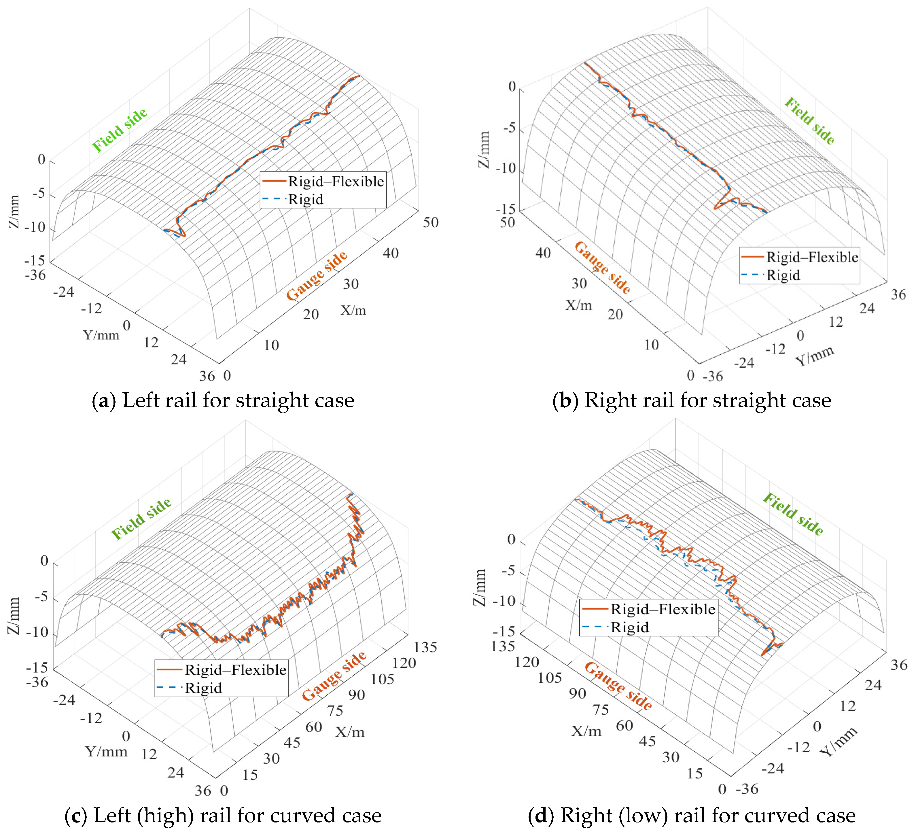
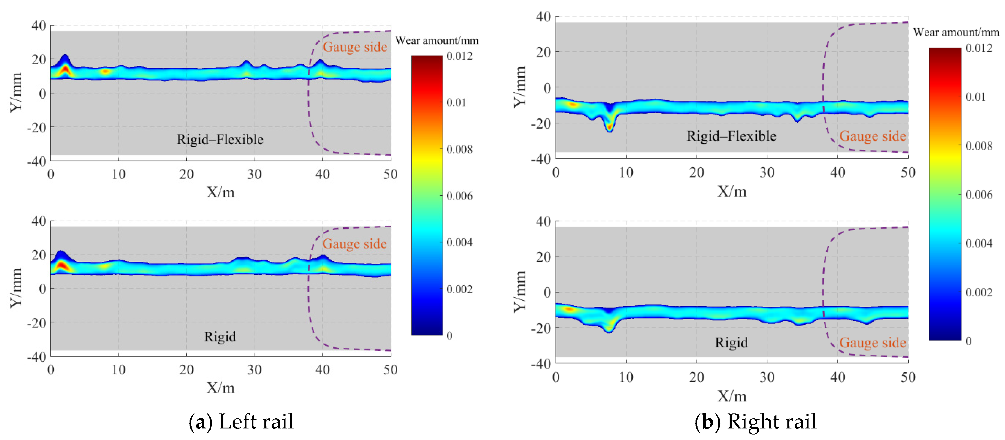
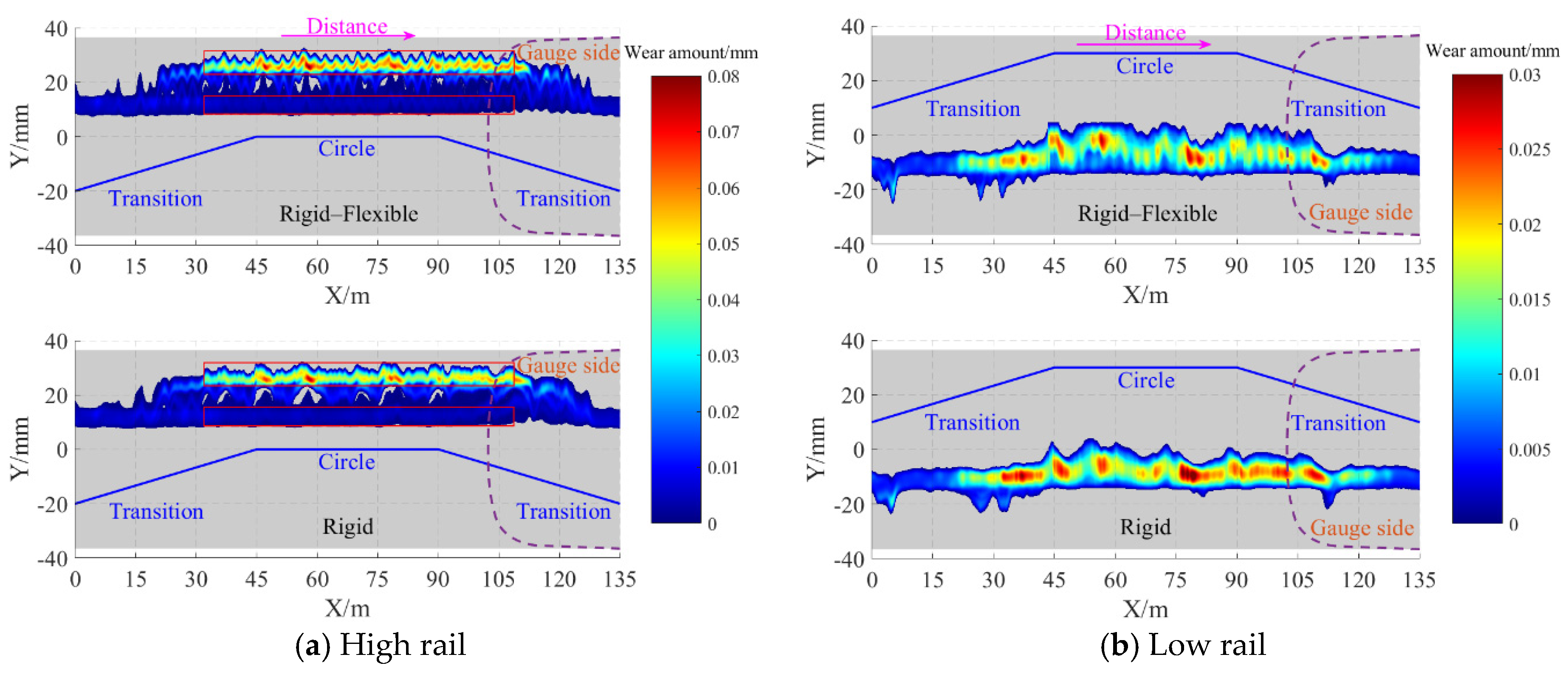
4.2. Three-Dimensional Wear Distribution of Rail
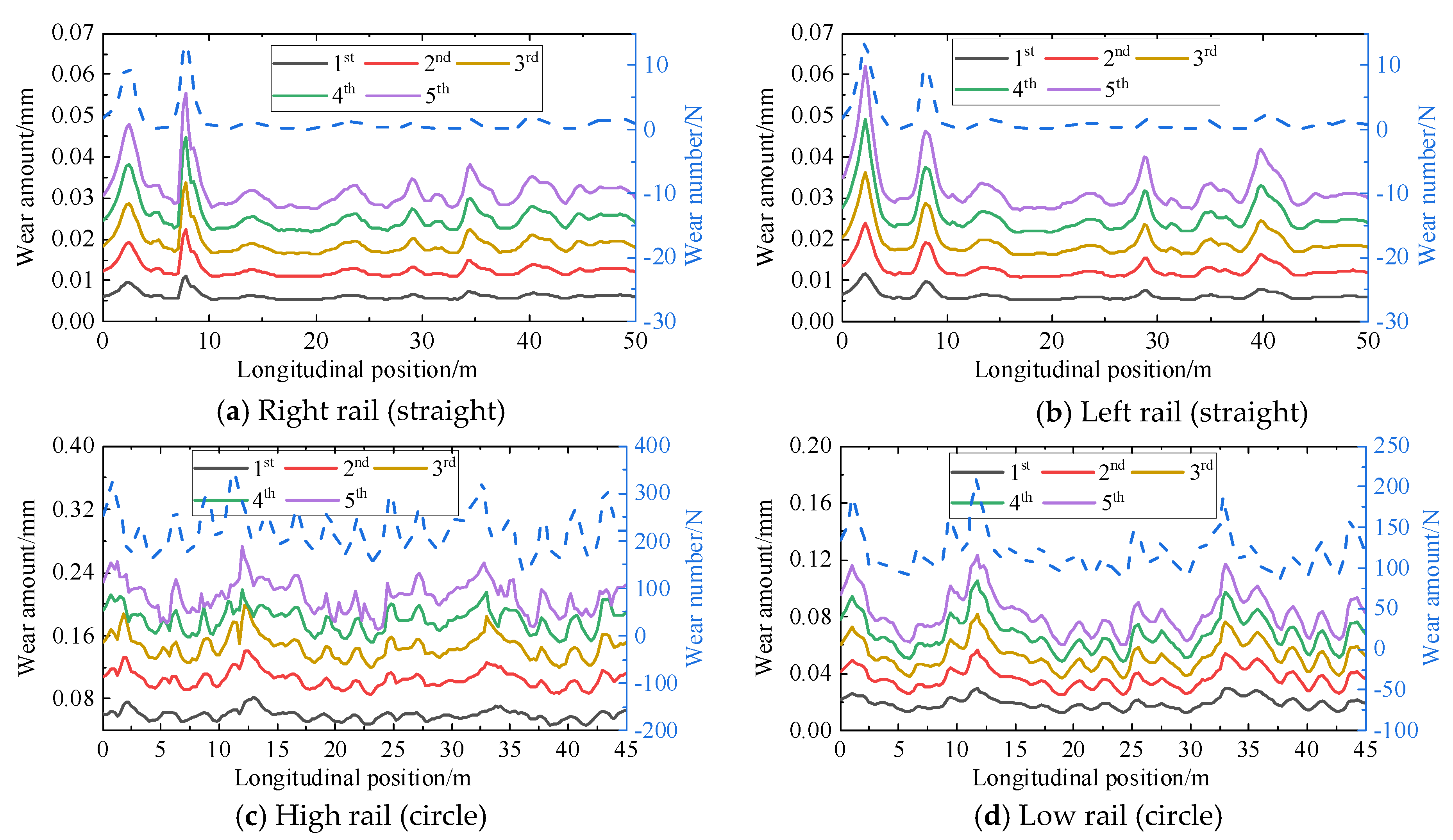
4.3. Rail Lateral Wear Distribution
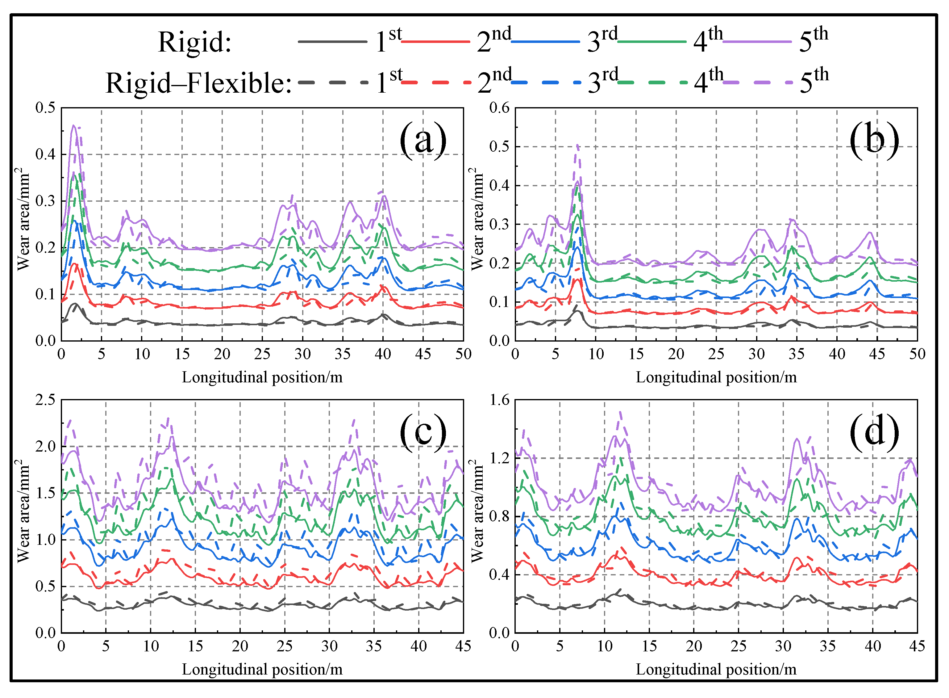
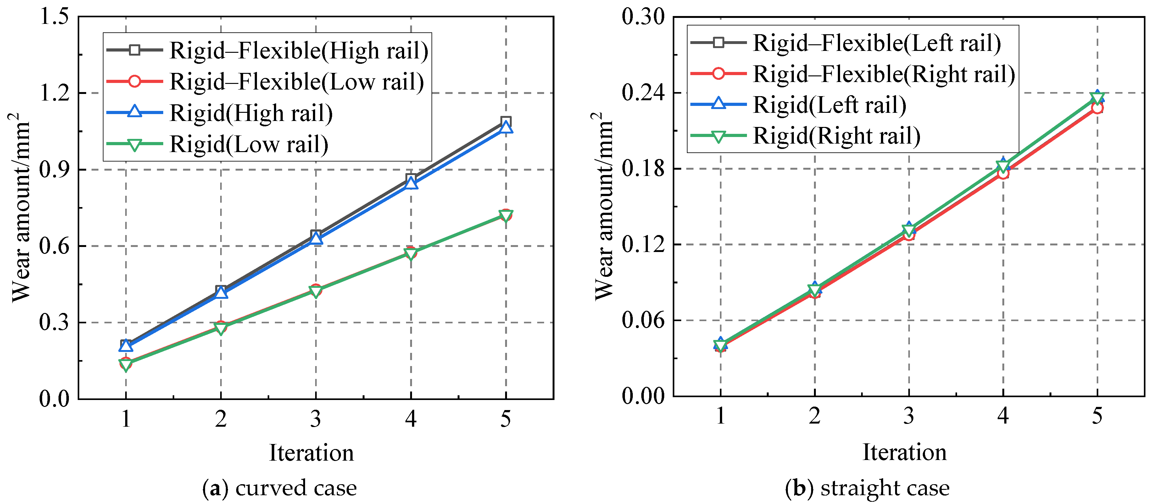
4.4. Wear Area
5. Conclusions
- (1)
- For the case of straight track, the difference between the calculated positions of the rail contact points with the two models is relatively insignificant. In curves with small radius, some discrepancy is observed. This discrepancy can be attributed to the fact that the rigid-flexible coupled dynamic model takes into account the dynamic expansion of the track gauge, which, in turn, causes a larger lateral displacement of the wheelset compared to the multi-rigid-body dynamic model.
- (2)
- The two models show relative similarity in terms of the three-dimensional wear distribution of the rail, with consistent prominent wear regions observed. The main difference between the two models is in the depth and range of wear, while the shape of the lateral wear distribution and overall wear characteristics remain essentially the same. In the first five iterations, the maximum percentage difference in the average wear area between the two models is 3.4% for the curved and straight track and 3.6% for the straight track.
- (3)
- The track irregularity is the main reason for the uneven distribution of rail wear in the longitudinal direction. The wear band on the straight and circular tracks is relatively straight in the longitudinal direction. At the transition, differences in radius of curvature and superelevation at different longitudinal positions result in a trumpet-shaped wear band, and the region near the circular curve has higher wear and a wider wear range. The maximum wear depth and wear area on each cross section exhibit a robust correlation with the wear number at the corresponding location. In addition, the areas of pronounced wear remain almost unchanged as the wear progresses.
- (4)
- Considering the computational efficiency and accuracy, it is advisable to use a multi-rigid-body dynamic model to predict the rail wear.
Author Contributions
Funding
Data Availability Statement
Conflicts of Interest
References
- Jin, X. Research progress of high-speed wheel–rail relationship. Lubricants 2022, 10, 248. [Google Scholar] [CrossRef]
- Wang, S.; Qian, Y.; Feng, Q.; Guo, F.; Rizos, D.; Luo, X. Investigating high rail side wear in urban transit track through numerical simulation and field monitoring. Wear 2021, 470, 203643. [Google Scholar] [CrossRef]
- Venter, J.P. Investigation into the abnormally high wear rate of AC electric locomotive wheels on the Ermelo-Richards Bay coal line when replacing UIC-A rail with chrome-maganese rail. In Proceedings of the Fourth International Heavy Haul Railway Conference 1989: Railways in Action, Brisbane, Australia, 11–15 September 1989; pp. 551–556. [Google Scholar]
- Bosso, N.; Magelli, M.; Zampieri, N. Simulation of wheel and rail profile wear: A review of numerical models. Rail. Eng. Sci. 2022, 30, 403–436. [Google Scholar] [CrossRef]
- Shebani, A.; Iwnicki, S. Prediction of wheel and rail wear under different contact conditions using artificial neural networks. Wear 2018, 406, 173–184. [Google Scholar] [CrossRef]
- Han, P.; Zhang, W. A new binary wheel wear prediction model based on statistical method and the demonstration. Wear 2015, 324, 90–99. [Google Scholar] [CrossRef]
- Jendel, T. Prediction of wheel profile wear—Comparisons with field measurements. Wear 2002, 253, 89–99. [Google Scholar] [CrossRef]
- Enblom, R.; Berg, M. Proposed procedure and trial simulation of rail profile evolution due to uniform wear. Proc. Inst. Mech. Eng. Part F J. Rail Rapid Transit. 2008, 222, 15–25. [Google Scholar] [CrossRef]
- Jin, X.; Xiao, X.; Wen, Z.; Guo, J.; Zhu, M. An investigation into the effect of train curving on wear and contact stresses of wheel and rail. Tribol. Int. 2009, 42, 475–490. [Google Scholar] [CrossRef]
- Ye, Y.; Sun, Y.; Shi, D.; Peng, B.; Hecht, M. A wheel wear prediction model of non-Hertzian wheel–rail contact considering wheelset yaw: Comparison between simulated and field test results. Wear 2021, 474, 203715. [Google Scholar] [CrossRef]
- Zhu, A.; Yang, S.; Li, Q.; Yang, J.; Li, X.; Xie, Y. Simulation and measurement study of metro wheel wear based on the Archard model. Ind. Lubr. Tribol. 2018, 71, 284–294. [Google Scholar] [CrossRef]
- Zhu, A.; Yang, S.; Li, Q.; Yang, J.; Fu, C.; Zhang, J.; Yao, D. Research on prediction of metro wheel wear based on integrated data-model-driven approach. IEEE Access 2019, 7, 178153–178166. [Google Scholar] [CrossRef]
- Ding, J.; Li, F.; Huang, Y.; Sun, S.; Zhang, L. Application of the semi-Hertzian method to the prediction of wheel wear in heavy haul freight car. Wear 2014, 314, 104–110. [Google Scholar] [CrossRef]
- Wen, B.; Wang, S.; Tao, G.; Li, J.; Ren, D.; Wen, Z. Prediction of rail profile evolution on metro curved tracks: Wear model and validation. Int. J. Rail Transp. 2022, 1–22. [Google Scholar] [CrossRef]
- Li, Y.; Ren, Z.; Enblom, R.; Stichel, S.; Li, G. Wheel wear prediction on a high-speed train in China. Veh. Syst. Dyn. 2020, 58, 1839–1858. [Google Scholar] [CrossRef]
- Innocenti, A.; Marini, L.; Meli, E.; Pallini, G.; Rindi, A. Prediction of wheel and rail profile wear on complex railway networks. Int. J. Rail Transp. 2014, 2, 111–145. [Google Scholar] [CrossRef]
- Hartwich, D.; Müller, G.; Meierhofer, A.; Obadic, D.; Rosenberger, M.; Lewis, R.; Six, K. A new hybrid approach to predict worn wheel profile shapes. Veh. Syst. Dyn. 2022, 1–17. [Google Scholar] [CrossRef]
- Ye, Y.; Qi, Y.; Shi, D.; Sun, Y.; Zhou, Y.; Hecht, M. Rotary-scaling fine-tuning (RSFT) method for optimizing railway wheel profiles and its application to a locomotive. Rail. Eng. Sci. 2020, 28, 160–183. [Google Scholar] [CrossRef]
- Li, G.; Li, X.; Li, M.; Na, T.; Wu, S.; Ding, W. Multi-objective optimisation of high-speed rail profile with small radius curved based on NSGA-II Algorithm. Veh. Syst. Dyn. 2022, 1–25. [Google Scholar] [CrossRef]
- Shi, J.; Gao, Y.; Long, X.; Wang, Y. Optimizing rail profiles to improve metro vehicle-rail dynamic performance considering worn wheel profiles and curved tracks. Struct. Multidiscip. Optim. 2021, 63, 419–438. [Google Scholar] [CrossRef]
- Gao, T.; Wang, Q.; Yang, K.; Yang, C.; Wang, P.; He, Q. Estimation of rail renewal period in small radius curveds: A data and mechanics integrated approach. Measurement 2021, 185, 110038. [Google Scholar] [CrossRef]
- Jin, X.; Wu, P.; Wen, Z. Effects of structure elastic deformations of wheelset and track on creep forces of wheel/rail in rolling contact. Wear 2002, 253, 247–256. [Google Scholar] [CrossRef]
- Zhai, W.; Wang, K.; Cai, C. Fundamentals of vehicle-track coupled dynamics. Veh. Syst. Dyn. 2009, 47, 1349–1376. [Google Scholar] [CrossRef]
- Aceituno, J.F.; Wang, P.; Wang, L.; Shabana, A.A. Influence of rail flexibility in a wheel/rail wear prediction model. Proc. Inst. Mech. Eng. Part F J. Rail Rapid Transit. 2017, 231, 57–74. [Google Scholar] [CrossRef]
- Tao, G.; Ren, D.; Wang, L.; Wen, Z.; Jin, X. Online prediction model for wheel wear considering track flexibility. Multibody Syst. Dyn. 2018, 44, 313–334. [Google Scholar] [CrossRef]
- Shi, Z.; Zhu, S.; Rindi, A.; Meli, E. Development and validation of a wear prediction model for railway applications including track flexibility. Wear 2021, 486, 204092. [Google Scholar] [CrossRef]
- Guo, T.; Qi, Y.; Gan, F. Simulation and analysis of wheel wear prediction with rigid flexible couple wheelset. Conf. Ser. Earth Environ. Sci. 2018, 189, 032012. [Google Scholar] [CrossRef]
- Vila, P.; Fayos, J.; Baeza, L. Simulation of the evolution of rail corrugation using a rotating flexible wheelset model. Veh. Syst. Dyn. 2011, 49, 1749–1769. [Google Scholar] [CrossRef]
- Baeza, L.; Vila, P.; Xie, G.; Iwnicki, S.D. Prediction of rail corrugation using a rotating flexible wheelset coupled with a flexible track model and a non-Hertzian/non-steady contact model. J. Sound Vib. 2011, 330, 4493–4507. [Google Scholar] [CrossRef]
- Kalker, J.J. A Fast Algorithm for the Simplified Theory of Rolling Contact. Veh. Syst. Dyn. 1982, 11, 1–13. [Google Scholar] [CrossRef]
- Guo, L. Study on Wear and Damage Behaviors and Wear Prediction of U75V Rail under Dry and Water Medium Conditions. Ph.D. Thesis, Southwest Jiaotong University, Chengdu, China, 2022. (In Chinese). [Google Scholar]
- Enblom, R.; Berg, M. Simulation of railway wheel profile development due to wear—Influence of disc braking and contact environment. Wear 2005, 258, 1055–1063. [Google Scholar] [CrossRef]
- Braghin, F.; Lewis, R.; Dwyer-Joyce, R.S.; Bruni, S. A mathematical model to predict railway wheel profile evolution due to wear. Wear 2006, 261, 1253–1264. [Google Scholar] [CrossRef]
- Lewis, R.; Dwyer-Joyce, R.S. Wear mechanisms and transitions in railway wheel steels. J. Eng. Tribol. 2004, 218, 467–478. [Google Scholar] [CrossRef]
- Lewis, R.; Olofsson, U. Mapping rail wear regimes and transitions. Wear 2004, 257, 721–729. [Google Scholar] [CrossRef]
- Sun, Y.; Guo, Y.; Lv, K.; Chen, M.; Zhai, W. Effect of hollow-worn wheels on the evolution of rail wear. Wear 2019, 436, 203032. [Google Scholar] [CrossRef]
- Sun, Y.; Guo, Y.; Zhai, W. Prediction of rail non-uniform wear—Influence of track random irregularity. Wear 2019, 420, 235–244. [Google Scholar] [CrossRef]
- Guyan, R.J. Reduction of stiffness and mass matrices. AIAA J. 1965, 3, 380. [Google Scholar] [CrossRef]


| Parameter | Value | Units |
|---|---|---|
| Car body mass (AW0/AW3) | 25,640/50,650 | kg |
| Bogie mass | 2800 | kg |
| Wheelset mass | 1140 | kg |
| Primary spring longitudinal stiffness | 1.4 | MN/m |
| Primary spring lateral stiffness | 6.5 | MN/m |
| Primary spring vertical stiffness | 1.1 | MN/m |
| Primary vertical damper stiffness | 6.4 | MN/m |
| Air spring longitudinal stiffness | 0.12 | MN/m |
| Air spring lateral stiffness | 0.12 | MN/m |
| Secondary vertical damper stiffness | 8 | MN/m |
| Traction rod longitudinal stiffness | 13.6 | MN/m |
| Anti-roll bar roll angle stiffness | 1.5 | MNm/rad |
| Wheelbase | 2.5 | m |
| Wheel rolling-circle diameter | 0.84 | m |
| Mode Descriptions (Order) | Original Model (Hz) | Substructure (Hz) | Relative Error (%) | Mode Shapes |
|---|---|---|---|---|
| 1st Torsion (1) | 88.914 | 88.93 | 0.02 |  |
| 1st Bending (2 and 3) | 104.953/104.954 | 104.993/104.994 | 0.04/0.04 |  |
| 2nd Bending (4 and 5) | 201.001/201.003 | 201.252/201.253 | 0.12/0.12 | 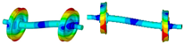 |
| Umbrella deformation (6) | 381.06 | 382.604 | 0.41 |  |
| Parameters | Value | Unit |
|---|---|---|
| Fastener spacing | 0.6 | m |
| Slab support spacing | 0.6 | m |
| Rail | 60 | kg/m |
| Young’s modulus of slab | 32.5 | GPa |
| Poisson’s ratio of slab | 0.24 | - |
| Density of slab | 2400 | kg/m3 |
| Fastener vertical stiffness | 60 | MN/m |
| Fastener vertical damping | 60 | kN·s/m |
| Slab support vertical stiffness | 170 | MN/m |
| Slab support vertical damping | 31 | kN·s/m |
Disclaimer/Publisher’s Note: The statements, opinions and data contained in all publications are solely those of the individual author(s) and contributor(s) and not of MDPI and/or the editor(s). MDPI and/or the editor(s) disclaim responsibility for any injury to people or property resulting from any ideas, methods, instructions or products referred to in the content. |
© 2023 by the authors. Licensee MDPI, Basel, Switzerland. This article is an open access article distributed under the terms and conditions of the Creative Commons Attribution (CC BY) license (https://creativecommons.org/licenses/by/4.0/).
Share and Cite
Wen, B.; Tao, G.; Wen, X.; Wang, S.; Wen, Z. Effect of Structural Flexibility of Wheelset/Track on Rail Wear. Lubricants 2023, 11, 231. https://doi.org/10.3390/lubricants11050231
Wen B, Tao G, Wen X, Wang S, Wen Z. Effect of Structural Flexibility of Wheelset/Track on Rail Wear. Lubricants. 2023; 11(5):231. https://doi.org/10.3390/lubricants11050231
Chicago/Turabian StyleWen, Bingguang, Gongquan Tao, Xuguang Wen, Shenghua Wang, and Zefeng Wen. 2023. "Effect of Structural Flexibility of Wheelset/Track on Rail Wear" Lubricants 11, no. 5: 231. https://doi.org/10.3390/lubricants11050231