Abstract
The thermal analysis of brake discs is crucial for studying issues such as wear and cracking. This paper establishes a symmetric two-dimensional brake disc model using the barycentric rational interpolation collocation method (BRICM). The model accounts for the effects of thermal radiation and is linearized using Newton’s linear iteration method. In the spatial dimension, the two-dimensional heat conduction equation is discretized using BRICM, while in the temporal dimension, it is discretized using the finite difference method (FDM). The resulting temperature distribution of the brake disc during two consecutive braking events is consistent with experimental data. Additionally, factors affecting the accurate calculation of the temperature are examined. Compared to other models, the proposed model achieves accurate temperature distributions with fewer nodes. Furthermore, the numerical results highlight the significance of thermal radiation within the model. The results obtained using BRICM can be used to predict the two-dimensional temperature distribution of train brake discs.
1. Introduction
The braking process of a train is a process of friction heat generation. The kinetic energy of the train is converted into heat energy due to the friction between the brake disc and the brake pad. The large amount of heat produced by friction can arouse high temperatures in the brake disc, resulting in a large temperature gradient and thermal expansion in the brake disc. Due to the restraint, the brake disc will be subjected to huge thermal stress, resulting in the deformation of the brake disc. Once the thermal and mechanical stresses in the brake disc exceed the ultimate bearing capacity of the material, thermal cracks and hot spots will be generated on the surface of the brake disc, as shown in Figure 1. Therefore, it is necessary to analyze the temperature field of train brake discs.
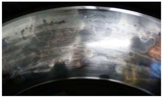
Figure 1.
Hot spots on the friction surface of forged brake discs on trains [1].
In order to obtain the temperature field distribution of brake discs, researchers have carried out a lot of work, and different numerical methods have been applied. To obtain the axial temperature field and temperature stress of the friction system composed of brake discs, Yevtushenko and Kuciej [2] obtained the analytic solution of the parabolic boundary value problem of heat conduction by the integral Laplace transform technique. The verification of analytical solutions with experimental data showed that such solutions were sufficiently good in the approximation calculation of the average temperature in the braking systems [3]. Based on the one-dimensional unsteady thermal model, Qi and Day [4] studied the temperature of the friction surface of aircraft brake carbon discs. Yang et al. [5] used the MOL (method of lines) to solve the one-dimensional friction heat conduction boundary value problem, and they obtained the braking temperature of the brake disc when the train was braking twice in a row with a velocity-related friction coefficient and the long ramp. Lee [6] proposed a two-dimensional brake disc model to study the influence of the finite brake disc thickness on the thermoelastic instability through the equivalent Fourier Transform. Yevtushenko and Grzes [7] carried out finite element analysis on a single braking process to solve the axisymmetric problem of friction heat conduction in a pad/disc braking system, and they obtained the temperature distribution law and wear change curve of brake disc models with two different materials. Grzes [8] established the HDFW (equations of heat dynamics of friction and wear) equation system for the single braking process of a pad friction system, numerically solving these problems by using the finite element method. Under the action of uniform heat flow and rotating heat flow, Adamowicz and Grzes [9,10] studied the temperature distribution of 2D and 3D brake disc surfaces under single braking and repetitive braking using finite element technology.
On the other hand, many numerical methods have been successfully applied to solve the temperature field of brake discs, such as the finite difference method (FDM) [11], finite volume method (FVM), and finite element method (FEM) [12,13,14]. Since the FEM can consider the actual structure of the brake disc, the temperature field distribution is more consistent with the actual situation. However, the calculation process will consume a lot of time and cannot be integrated into the simulation of vehicle track coupling dynamic systems, which can provide braking energy under actual operating conditions [5]. Therefore, a meshless method can be applied to solve the friction heat conduction problem. Floater and Hormann [15] proposed a high-order barycentric rational interpolation collocation method, which has the advantages of high accuracy, fast speed and less nodes. In this method, differential matrices are generated on nodes of different dimensions of the equation, and the solution of the equation can be obtained by solving linear equations. Many researchers have successfully applied this method to solve partial differential equations, such as the nonlinear Korteweg–De Vries–Burgers equation [16], Fredholm–Volterra integral equation [16,17,18], Vibration equation [19,20,21], and heat conduction equation [22]. However, the solutions available in the literature are limited to theoretical studies and fail to solve complicated engineering problems, such as the friction heat of brake discs.
To obtain the friction heat of train brake discs, the BRICM is applied to solve the two-dimensional heat conduction equation of the brake disc in this paper, which considers the heat radiation in the boundary conditions. In the present model, the fourth power function of temperature is used to simulate the heat radiation [23], which is linearized by the newton linear iteration method [24]. In addition, since the two-dimensional heat conduction equation is a second-order, multi-dimensional, and nonlinear differential equation, the BRICM is used to discretize the equation directly. However, it will introduce a large calculation matrix, resulting in a slow calculation speed. Therefore, some improvements to the BRICM need to be made. In this paper, the FDM can be introduced to discretize the time dimension of the equation and the BRICM can be used to discretize the spatial dimension of the equation.
The organization of this paper is as follows. Firstly, the mathematical model of two-dimensional axisymmetric brake discs is established. Secondly, the BRICM and FDM are used to obtain the numerical solutions of the model. Next, the numerical results are verified with the experimental data and the published methods. After that, the effects of different numbers of nodes and different heat radiation treatment methods on the temperature of the brake disc are investigated. Finally, the axial and radial temperature distribution of the brake disc when braking twice consecutively are obtained.
2. Numerical Model of the Two-Dimensional Axisymmetric Brake Disc
2.1. Descriptions of the Numerical Model
Due to the axial symmetry of the brake disc structure, the brake disc can be simplified into a two-dimensional axisymmetric brake disc model, as shown in Figure 2. The brake disc system is composed of a brake disc and a brake pad. During braking, mechanical energy is converted into heat energy in the immediate area of the friction path between the brake disc and brake pad. The generated heat is dissipated by the axle, brake disc, and the exposed surface of the brake disc by heat conduction, heat convection, and heat radiation. During the whole braking process, the following assumptions are made:
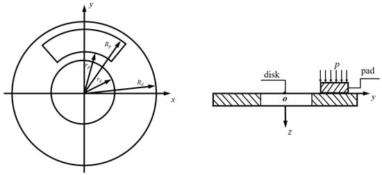
Figure 2.
Simplified schematic diagram of train brake disc.
- (1)
- The initial brake disc temperature and ambient temperature are Ta.
- (2)
- The braking pressure between the brake disc and the brake pad is constant.
- (3)
- The brake disc is homogeneous, and the material properties do not change with temperature.
- (4)
- The friction coefficient of the brake disc surface does not change with temperature.
- (5)
- The wear on the contact surface is negligible.
Based on the above assumptions, the two-dimensional axisymmetric heat conduction equation in cylindrical coordinate systems can be obtained [6].
where ρ is the material density of the brake disc; c is the specific heat capacity; λ is the thermal conductivity; rd is the radius of the inner ring of the brake disc; Rd is the radius of the outer ring of the brake disc; k is the thermal diffusivity; and d is the thickness of the brake disc. To solve Equation (1), it is necessary to give the initial boundary conditions of the friction heat conduction problem.
The temperature of the brake disc at the initial time of train braking is
Considering the heat radiation of the brake disc, the heat transfer boundary condition of the brake disc is satisfied.
When s = 0, the effect of thermal radiation is considered s = 1; the effect of thermal radiation is negligible; h is the convective heat transfer coefficient; εb = 0.35 and εk = 0.95 are the emissivity; subscripts k and b represent the friction surface and heat dissipation rib surface; σ = 5.67 × 10⁻⁸ is the Boltzmanns constant; rp is the radius of the inner ring of the brake pad; Rp is the radius of the outer ring of the brake pad; and q(t) is the friction heat flow, which is given by Equation (4).
where f is the friction coefficient of the brake disc surface; w(t) is the rotation speed of the brake disc; η is the heat flow distribution rate [8]; and p0 is the pressure on the brake disc.
where subscripts d and p are the brake disc and brake pad, respectively; m is the braking mass; a is the braking deceleration; R is the radius of wheel; S is Friction ring area; and rf is the friction equivalent radius.
2.2. BRICM for the Mathematical Model
The heat conduction equation of the two-dimensional axisymmetric brake disc is discretized by BRICM and FDM.
The temperature field is T(z,r,t), and the braking time is t = [0, ts]. At t = tN+1, the finite difference method is used to discretize the time dimension of the heat conduction equation with K points.
where and are the second derivative of the temperature function with z and r at t = tN+1, respectively and is the first derivative of the temperature function with r.
For the spatial dimension, the intervals z = [0, d] and r = [rd, Rd] are discretized into m and n nodes, respectively. The sketch of the calculation domain is shown in Figure 3.
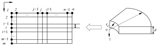
Figure 3.
Sketch of the discretization of the brake disc in the axial direction and radial direction.
The thickness z is discretized into m points, 0 = z1 < z2 < …< zm = d. The radius r is discretized into n points, rd = r1 < r2 < …< rn = Rd. The m×n tensor-type calculation nodes of the region are (zi, rj), i = 1, 2, …, m. The barycentric rational interpolation equation of the brake disc temperature field function can be expressed as
where and Li(z) and Mj(r) are the barycentric interpolation basis functions along the z direction and r direction [22]. Then, the heat conduction in Equation (6) can be described as follows:
Equation (8) can be written in the following simplified form:
where represents the Kronecker product of the matrix; Im and In are the m-order and n-order identity matrices; and L(2) are M(2) the second-order differential matrices on the node.
; ; ; ; ; .
In Equation (3), since the thermal radiation in the boundary conditions is highly nonlinear, it is difficult to calculate it directly. In this paper, the thermal radiation is linearized by the newton linear iteration method.
At the time t = tN+1, with a given initial function T0 = T0(z, r), the thermal radiation is expanded by the Taylor expansion.
Then, the boundary conditions can be obtained.
The discrete equation of Equation (11) is
where
where and represent the first row and the m-th row of the first-order differential matrix in the z direction; and represent the first row and the n-th row of the first-order differential matrix in the r direction; and represent the first row and the m-th row of the m-order unit matrix; and and represent the first row and the n-th row of the n-order unit matrix.
By solving Equations (9), (12) and (13), the temperature field distribution of two-dimensional axisymmetric brake discs with different heat radiation term treatment methods can be obtained.
3. Numerical Results and Discussion
3.1. Verification of Numerical Model
This section analyzes the transient temperature field generated by the friction heat load of the brake disc during single braking and braking twice consecutively. Firstly, the model is compared with results in [7], which ignores the effect of thermal radiation. Then, the experimental data are conducted to verify the model.
3.1.1. Comparisons with the FEM Results
The present method is firstly compared with the finite element results in [7] which ignores the thermal radiation. The evolutions of temperature on the contact surface of the disc during braking for the cast-iron disc and the pad made of FC-16L (retinax A) are shown in Figure 4. The initial braking angular velocity is w0 = 88.464 s−1, and the braking time is ts = 3.96 s; the heat transfer coefficient and friction coefficient do not change with the temperature.
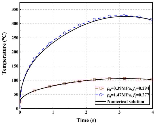
Figure 4.
Curve of brake disc surface temperature with time (z = 0 mm, r = 95 mm).
Figure 4 shows that the numerical results of the present model ignoring the thermal radiation are in good agreement with that of [7] in the cases of p0 = 0.39 MPa, f0 = 0.294 and p0 = 1.47 MPa, f0 = 0.277.
3.1.2. Experimental Verification
The test data were obtained on a Renk’s full-scale dynamometer test bench, which is shown in Figure 5. The test sample consists of a wheeled brake disc and brake calliper, which are placed in the test chamber to simulate the train operation environment. The temperature is measured by six thermocouples embedded 1 mm from the brake disc surface. The location of the test points is shown in Figure 6. This method can only obtain six continuous temperature points of the brake disc, and the average temperature of the six measuring points is taken as the temperature of the brake disc. In this test, the temperature of the brake disc for braking twice consecutively is tested, and the speed curve of the brake disc is shown in Figure 7.
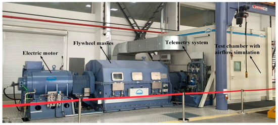
Figure 5.
Renk dynamometer test bench.
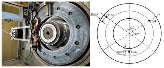
Figure 6.
Location of the test points.
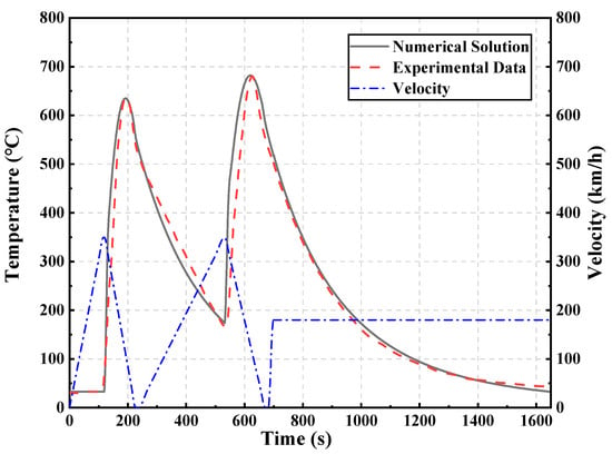
Figure 7.
Comparison of numerical solutions and experimental data.
The brake disc material is quenching and tempering steel coupled with ISOBAR sinter brake pad. The structural parameters and material parameters of the brake disc are shown in Table 1.

Table 1.
Structural parameters and properties of materials of the disc and the pad at 40 °C.
The uniform heat flow method is used to input energy to the brake disc. The average friction coefficient during braking is 0.31, and the clamping force of the brake calliper is constant at 36 kN. The values of other parameters are S = 0.16 m2, and the heat flow distribution coefficient is 0.84, the average convective coefficient on the friction surface side is 170 W/(m2·K), and the average convective coefficient on the heat dissipation rib side is 240 W/(m2·K).
Figure 7 shows that the average surface temperature of the brake disc obtained through the numerical solution is consistent with the experimental data. The temperature of the brake disc at the second brake is significantly higher than that at the first brake; the initial temperature can reach up to 160 °C, while that of the first brake application is 40 °C. The maximum average temperature of the brake disc surface is 635.05 °C and 681.75 °C, respectively. And the maximum average temperatures corresponding to the experimental data are 636.80 °C and 679.98 °C. It can be seen that the two maximum average temperatures of the numerical solution are the same as those of the test data.
The above results show that the numerical results of the two models with and without thermal radiation are in good agreement with the experimental data and the finite element results in the current numerical models, respectively.
3.2. Investigation on Factors Affecting Temperature
This part investigates the factors affecting temperature. Firstly, the influence of grid density on the calculation is investigated; that is, the effect of different numbers of nodes in the axial and radial directions, respectively. Secondly, the influence of thermal radiation treatment in boundary conditions on the temperature is investigated.
3.2.1. Effect of Mesh Density on the Temperature
Figure 8 and Figure 9 investigate the effect of different numbers of nodes in the axial and radial directions on the temperature of the brake disc under p0 = 1.47 MPa, f0 = 0.277.
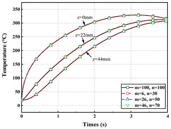
Figure 8.
Curve of brake disc temperature with time when the number of axial nodes m = 6, 26, 46, 100, the number of radial nodes n = 30, 50, 70, 100, and the number of time nodes K = 500 (r = 95 mm).
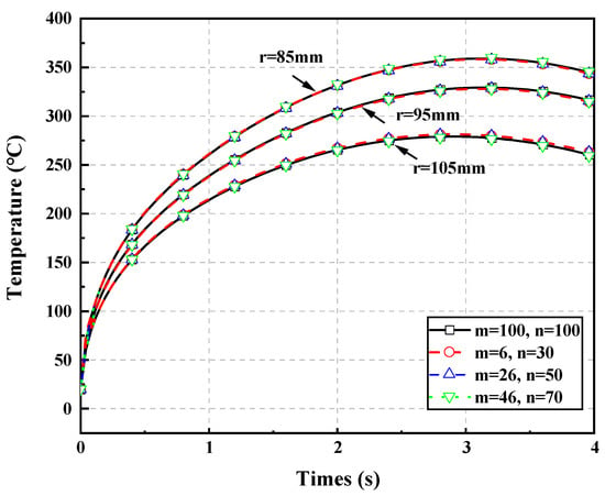
Figure 9.
Curve of brake disc surface temperature with time when the number of axial nodes m = 6, 26, 46, 100, the number of radial nodes n = 30, 50, 70, 100, and the number of time nodes K = 500 (z = 0 mm).
Figure 8 and Figure 9 show the temperature curves at different axial and radial positions of the brake disc when the grid density is m × k = 6 × 30, 26 × 50, 46 × 70, and 100 × 100. The results show that the grid densities have little effect on the distributions of temperature.
Take the temperature obtained from the grid density of 100 × 100 as the reference value to investigate the relative error of the temperature obtained from the other three grid densities. The relative error is expressed as , where is the temperature at point (z0, r0). Table 2 shows the calculation time and relative errors of the four grid densities.
Table 2.
Calculation time and relative error of temperature with different grid densities.
Table 2 shows the calculation time and temperature relative errors for different grid densities. The results show that the calculation time increases with the increase in mesh density, but the relative error does not change much. Therefore, less nodes can be used to calculate the temperature field, which can greatly reduce the calculation time.
From the above analysis, it can be concluded that the density of radial and axial nodes has little effect on the temperature in the present numerical model. Therefore, while the time node is K = 500, the temperature distribution of the brake disc can be obtained by fewer nodes in the axial and radial directions.
3.2.2. Effect of Boundary Conditions
The treatment of boundary conditions has a great influence on the temperature of the brake disc. In Equation (3), when s = 0, the influence of thermal radiation is considered, and when s = 1, the influence of thermal radiation is ignored. This part discusses the effect of the thermal radiation in the boundary conditions on the temperature field of the brake disc. The disc parameters and speed curve used in the numerical model are consistent with those used in the experiment.
Figure 10 shows the temperature curve of considering and neglecting thermal radiation in boundary conditions during two consecutive braking processes. During the first braking, the maximum average surface temperature of the brake disc is 635.05 °C and 642.15 °C, respectively, with a difference of 8.10 °C under the conditions of considering and ignoring the thermal radiation. During the second braking, the maximum average temperature of the brake disc surface is 681.75 °C and 703.24 °C, respectively, with a difference of 21.49 °C. It can be seen that in the consecutive braking process, thermal radiation has a great impact on the maximum average temperature of the surface of the brake disc. At the stage of the temperature rise, the two curves basically coincide. When the temperature drops, the heat absorbed by the brake disc is less than the heat dissipated. Ignoring the influence of heat radiation will cause the temperature of the brake disc to be higher than the actual temperature. Therefore, the thermal radiation should be considered in the model.
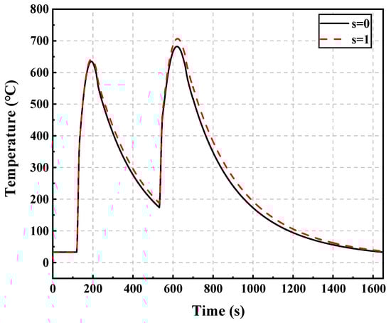
Figure 10.
Curve of brake disc surface temperature with time when s = 0 and s = 1 in boundary conditions.
3.3. Analysis of Brake Disc Temperature Field
Figure 11, Figure 12 and Figure 13 show the contour map of the axial and radial temperature of the brake disc with time and the temperature distribution diagram of the cross section of the brake disc at the maximum average temperature.
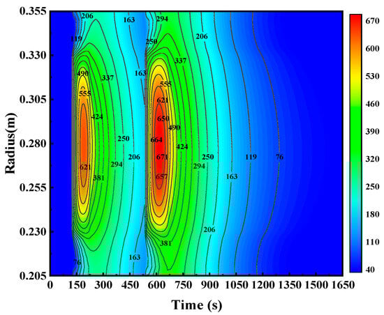
Figure 11.
Contour map of radial temperature of brake disc with time (°C).
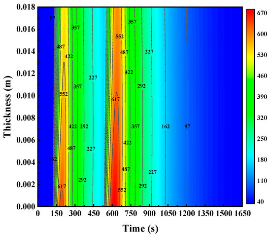
Figure 12.
Contour map of axial temperature of brake disc with time (°C).
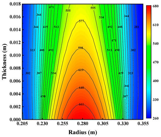
Figure 13.
Contour map of temperature distribution in radial section of brake disc at time of maximum temperature (°C).
As can be seen from Figure 11, along the radial direction, friction heat flow is generated on the contact surface between the brake disc and the brake pad and diffuses towards the inner diameter and outer diameter. Therefore, the radial temperature of the brake disc increases. During the first braking process, the temperature reaches the highest value on the friction surface. After that, the heat effect of diffusion is greater than that generated on the friction surface, resulting in a decrease in temperature. In the second braking process, since the initial temperature is the temperature after the natural cooling of the first braking, the maximum temperature in the second braking process is significantly higher than that in the first braking. The temperature distribution of the second braking process is the same as that of the first braking process. After braking, accelerate the brake disc to 180 km/h and keep it rotating at a constant speed so that the temperature of the brake disc surface decreases rapidly.
Figure 12 shows that the heat diffuses along the thickness direction from the friction surface during the first braking, which increases the temperature of the brake disc in the thickness direction. With the progress of braking, the temperature at the friction surface z = 0 mm is significantly higher than that at z = 18 mm. In addition, it can be seen from the isoline that the times taken to reach the same temperature along the thickness direction are different. The second braking process is the same as the first braking process, but the temperature is higher than the first braking process.
It can be seen from Figure 13, at the moment of the highest temperature, that the temperature of the radial section of the brake disc gradually decreases from the highest temperature at z = 0 mm to the inside of the brake disc. Since the thickness of the brake disc is much less than the radial thickness of the brake disc, the temperature of the brake disc increases rapidly in the thickness direction, and the temperature at z = 18 mm is higher than that at r = 355 mm. Moreover, in the thickness direction, the friction surface of the brake disc is affected by the friction heat flow, and the heat energy diffuses in the direction of z = 18 mm.
Overall, the above-mentioned results show that it is feasible to calculate the two-dimensional axisymmetric brake disc temperature field by using the BRICM.
4. Conclusions
In this paper, the friction heat generation of the two-dimensional axisymmetric brake disc of the train is studied, and the two-dimensional axisymmetric heat conduction equation is successfully solved by the BRICM and FDM. The thermal radiation term is linearized by the newton linear iteration method. In order to verify the correctness of the algorithm, the temperature of the brake disc in two consecutive braking processes and a single braking process is compared and verified with experimental data and the finite element results in [7]. The factors affecting the accurate calculation of temperature are investigated. The following conclusions are obtained:
- (1)
- The average temperature distribution curve calculated by the two-dimensional model is in good agreement with the experimental data and the finite element results. The results show that the BRICM can be applied to the friction heat problem in the braking process.
- (2)
- In the numerical calculation, a few calculation nodes can obtain the correct temperature curve. This shows that the BRICM can meet the demand of the real-time calculation of the brake disc temperature of the vehicle track coupling system. In addition, comparison results show that the newton linear iteration method can be used to deal with thermal radiation in the boundary conditions. And the thermal radiation cannot be ignored in the current model.
- (3)
- The temperature contour map calculated by the BRICM is in line with the actual situation. This shows that the results obtained by the BRICM can be used to simulate the temperature distribution of the two-dimensional brake disc.
Author Contributions
Conceptualization, B.W. and L.Y.; methodology, B.W. and Y.Z.; software, Y.Z.; validation, B.W., G.X. and Y.Z.; writing—original draft preparation, B.W. and Y.Z.; writing—review and editing, B.W. and Z.W.; visualization, Y.Z. and Z.W.; supervision, B.W., Q.S. and L.Y.; funding acquisition, B.W. All authors have read and agreed to the published version of the manuscript.
Funding
This research was funded by the National Nature Science Foundation of China (No. 52372391).
Data Availability Statement
The data presented in this study are available on request from the corresponding author. The data are not publicly available due to privacy or ethical restrictions.
Conflicts of Interest
The authors declare that they have no known competing financial interests or personal relationships that could have appeared to influence the work reported in this paper.
References
- Li, Z.Q.; Han, J.M.; Yang, Z.Y.; Pan, L.K. The effect of braking energy on the fatigue crack propagation in railway brake discs. Eng. Fail. Anal. 2014, 44, 272–284. [Google Scholar] [CrossRef]
- Yevtushenko, A.; Kuciej, M. Temperature and thermal stresses in a pad/disc during braking. Appl. Therm. Eng. 2010, 30, 354–359. [Google Scholar] [CrossRef][Green Version]
- Nosko, A.L.; Mozalev, V.V.; Nosko, A.P.; Suvorov, A.V.; Lebedeva, V.N. Calculation of temperature of carbon disks of aircraft brakes with account of heat exchange with the environment. J. Frict. Wear 2012, 33, 233–238. [Google Scholar] [CrossRef]
- Qi, H.S.; Day, A.J. Investigation of disc/pad interface temperatures in friction braking. Wear 2007, 262, 505–513. [Google Scholar] [CrossRef]
- Yang, Y.Q.; Wu, B.; Shen, Q.; Xiao, G.W. Numerical simulation of the frictional heat problem of subway brake discs considering variable friction coefficient and slope track. Eng. Fail. Anal. 2021, 130, 105794. [Google Scholar] [CrossRef]
- Lee, K. Frictionally excited thermoelastic instability in automotive drum brakes. J. Tribol.-T Asme 2000, 122, 849–855. [Google Scholar] [CrossRef]
- Yevtushenko, A.A.; Grzes, P. Axisymmetric FEA of temperature in a pad/disc brake system at temperature-dependent coefficients of friction and wear. Int. Commun. Heat. Mass. 2012, 39, 1045–1053. [Google Scholar] [CrossRef]
- Grzes, P. Determination of the maximum temperature at single braking from the FE solution of heat dynamics of friction and wear system of equations. Numer. Heat Transf. A-Appl. 2017, 71, 737–753. [Google Scholar] [CrossRef]
- Adamowicz, A.; Grzes, P. Analysis of disc brake temperature distribution during single braking under non-axisymmetric load. Appl. Therm. Eng. 2011, 31, 1003–1012. [Google Scholar] [CrossRef]
- Adamowicz, A.; Grzes, P. Influence of convective cooling on a disc brake temperature distribution during repetitive braking. Appl. Therm. Eng. 2011, 31, 2177–2185. [Google Scholar] [CrossRef]
- Kazem, S.; Dehghan, M. Application of finite difference method of lines on the heat equation. Numer. Meth Part. D Equ. 2018, 34, 626–660. [Google Scholar] [CrossRef]
- Grzes, P.; Oliferuk, W.; Adamowicz, A.; Kochanowski, K.; Wasilewski, P.; Yevtushenko, A.A. The numerical-experimental scheme for the analysis of temperature field in a pad-disc braking system of a railway vehicle at single braking. Int. Commun. Heat Mass. 2016, 75, 1–6. [Google Scholar] [CrossRef]
- Yevtushenko, A.A.; Grzes, P. Mutual influence of the velocity and temperature in the axisymmetric FE model of a disc brake. Int. Commun. Heat Mass. 2014, 57, 341–346. [Google Scholar] [CrossRef]
- Yevtushenko, A.A.; Kuciej, M.; Grzes, P.; Wasilewski, P. Temperature in the railway disc brake at a repetitive short-term mode of braking. Int. Commun. Heat Mass. 2017, 84, 102–109. [Google Scholar] [CrossRef]
- Floater, M.S.; Hormann, K. Barycentric rational interpolation with no poles and high rates of approximation. Numer. Math. 2007, 107, 315–331. [Google Scholar] [CrossRef]
- Liu, H.Y.; Huang, J.; Pan, Y.B.; Zhang, J.P. Barycentric interpolation collocation methods for solving linear and nonlinear high-dimensional Fredholm integral equations. J. Comput. Appl. Math. 2018, 327, 141–154. [Google Scholar] [CrossRef]
- Li, J.; Cheng, Y.L. Linear barycentric rational collocation method for solving second-order Volterra integro-differential equation. Comput. Appl. Math. 2020, 39, 92. [Google Scholar] [CrossRef]
- Liu, H.; Huang, J. Numerical solution of special 2D Fredholm-Volterra integral equations using barycentric Gegenbauer interpolation collocation method. J. Phys. Conf. Ser. 2020, 1634, 012099. [Google Scholar] [CrossRef]
- Wu, H.; Wang, Y.; Zhang, W.; Wen, T. The barycentric interpolation collocation method for a class of nonlinear vibration systems. J. Low Freq. Noise Vib. Act. Control 2019, 38, 1495–1504. [Google Scholar] [CrossRef]
- Zhuang, M.L.; Miao, C.Q.; Ji, S.Y. Plane elasticity problems by barycentric rational interpolation collocation method and a regular domain method. Int. J. Numer. Meth. Eng. 2020, 121, 4134–4156. [Google Scholar] [CrossRef]
- Zhuang, M.L.; Miao, C.Q.; Wan, C.H. A Highly Accurate Collocation Method for Linear and Nonlinear Vibration Problems of Multi-Degree-Of-Freedom Systems Based on Barycentric Interpolation. Int. J. Nonlinear Sci. Numer. 2019, 20, 543–550. [Google Scholar] [CrossRef]
- Li, S.; Wang, Z. High Precision Meshless Barycenter Interpolation Collocation Method; Science Press: Beijing, China, 2012. [Google Scholar]
- Yang, S.M.; Tao, W.Q. Heat Transfer; Higher Education Press: Beijing, China, 2006. [Google Scholar]
- Li, S.; Wang, Z. Barycentric Interpolation Collocation Method for Nonlinear Problems; National Defense Industry Press: Beijing, China, 2015. [Google Scholar]


Disclaimer/Publisher’s Note: The statements, opinions and data contained in all publications are solely those of the individual author(s) and contributor(s) and not of MDPI and/or the editor(s). MDPI and/or the editor(s) disclaim responsibility for any injury to people or property resulting from any ideas, methods, instructions or products referred to in the content. |
© 2024 by the authors. Licensee MDPI, Basel, Switzerland. This article is an open access article distributed under the terms and conditions of the Creative Commons Attribution (CC BY) license (https://creativecommons.org/licenses/by/4.0/).