The Impact of Oil Viscosity and Fuel Quality on Internal Combustion Engine Performance and Emissions: An Experimental Approach

 ,
, 
Abstract
1. Introduction
2. Materials and Methods
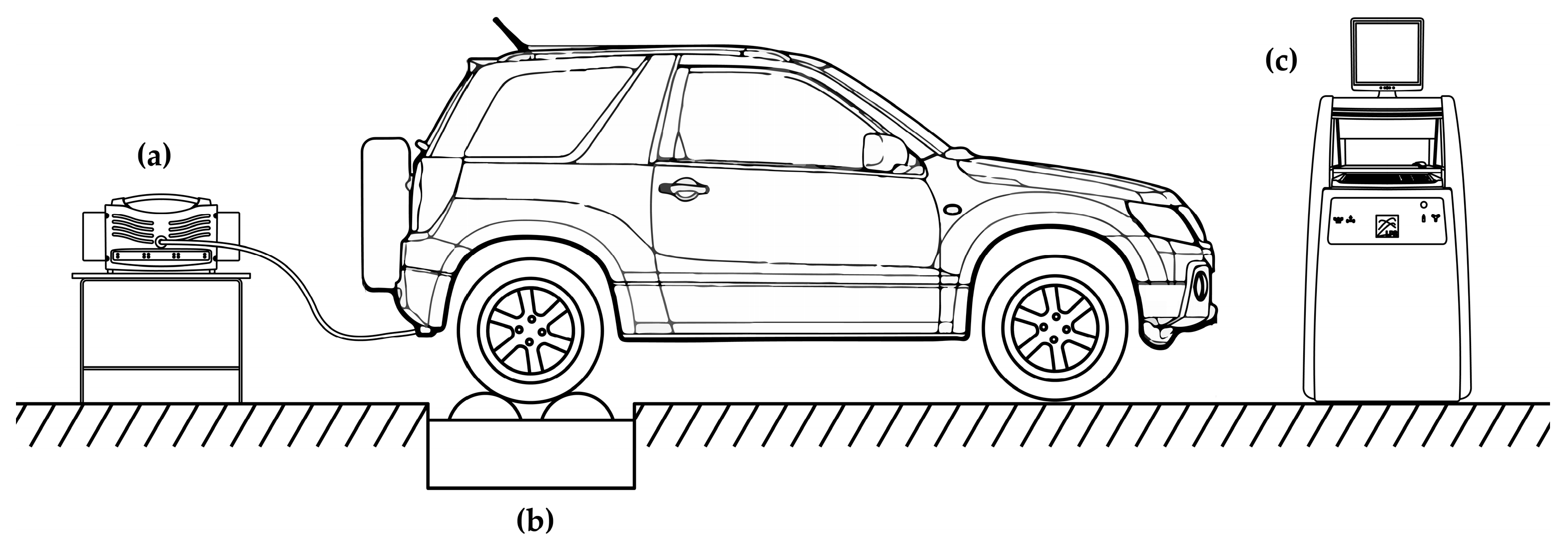
2.1. Experimental Setup Description
- Lower level: Ecopaís gasoline (−1).
- Medium level: Super gasoline (0).
- Upper level: Super gasoline with an octane booster additive (1).
2.2. Response Surface Methodology
3. Results
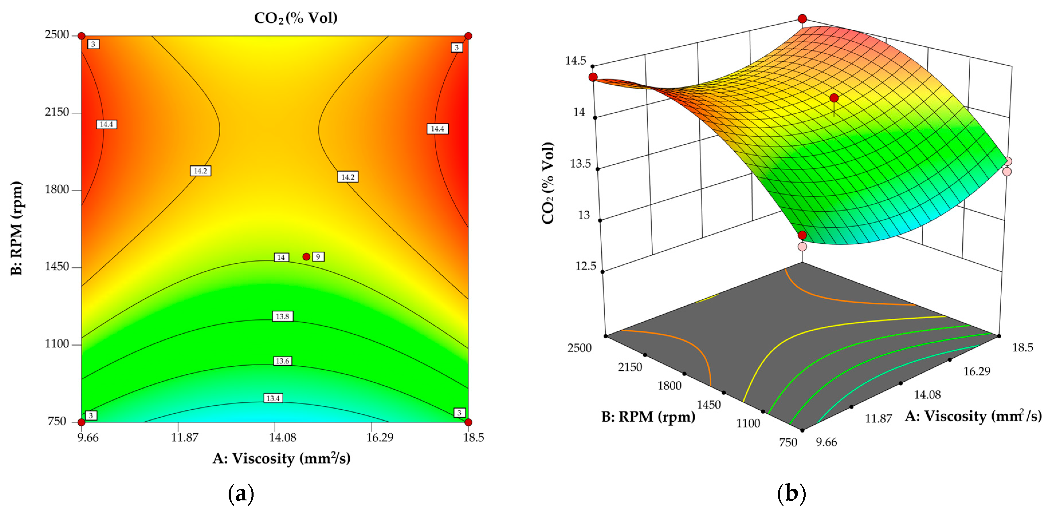
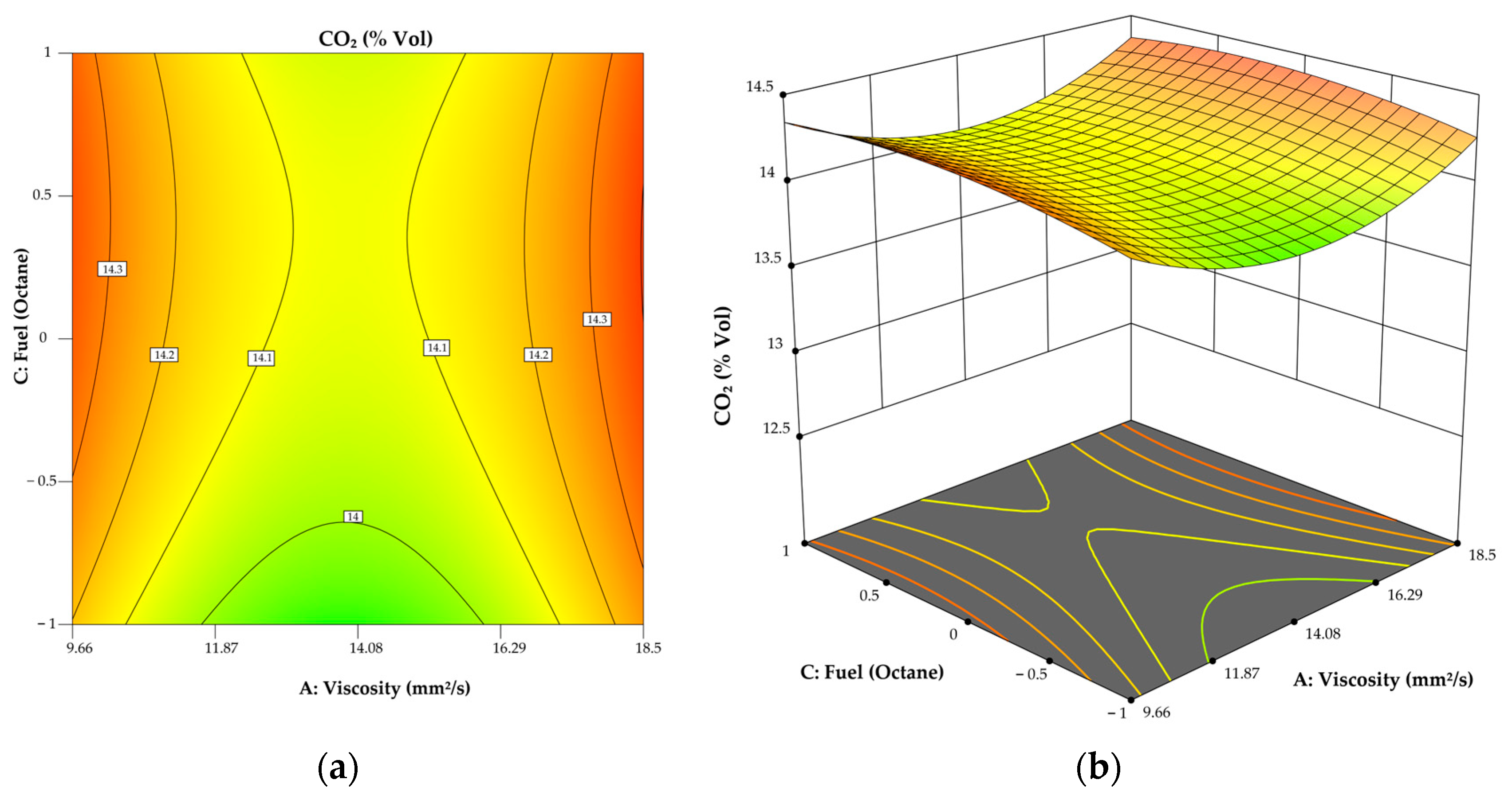
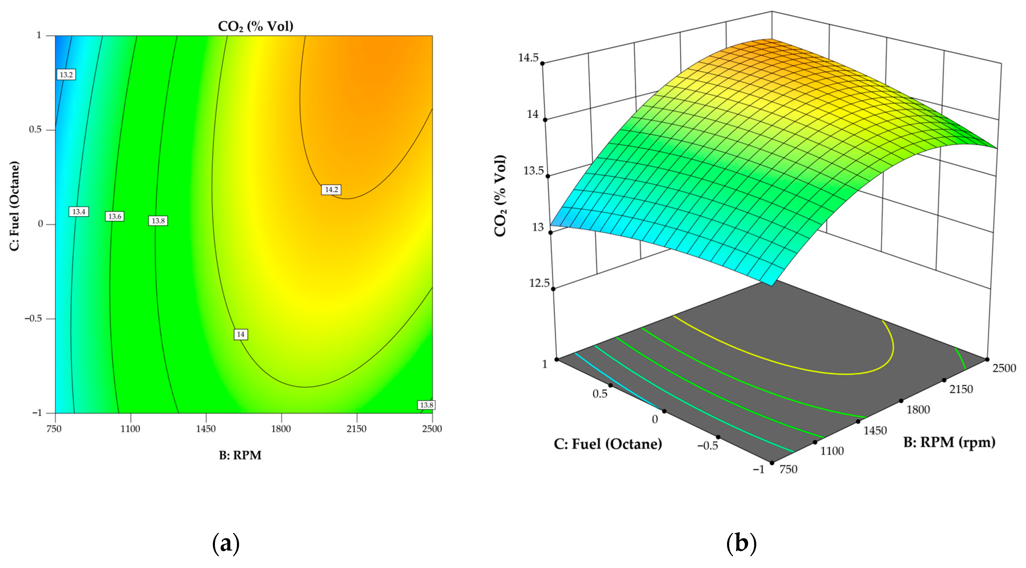
3.1. Model for CO2
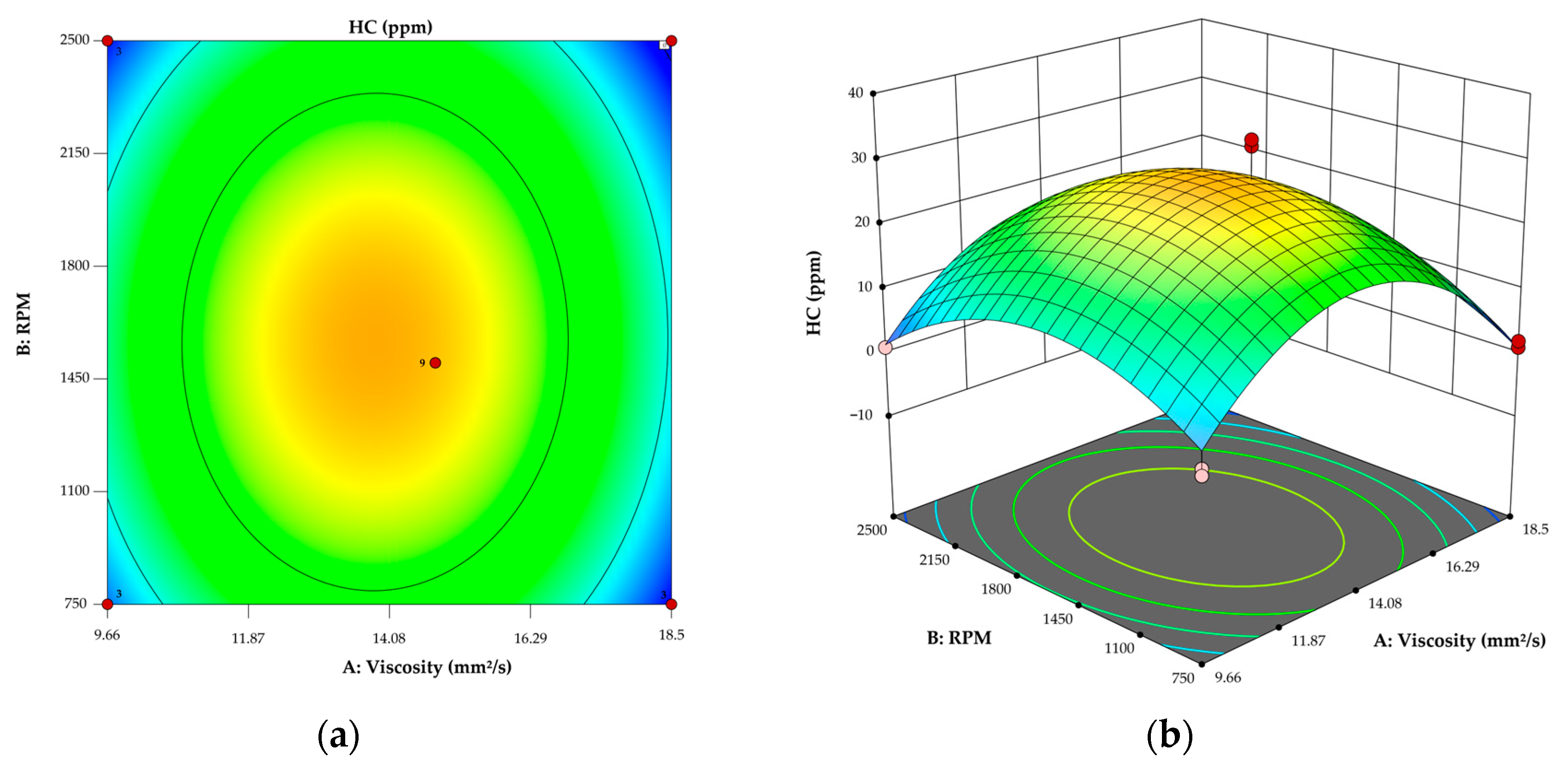
3.2. Model for HCs
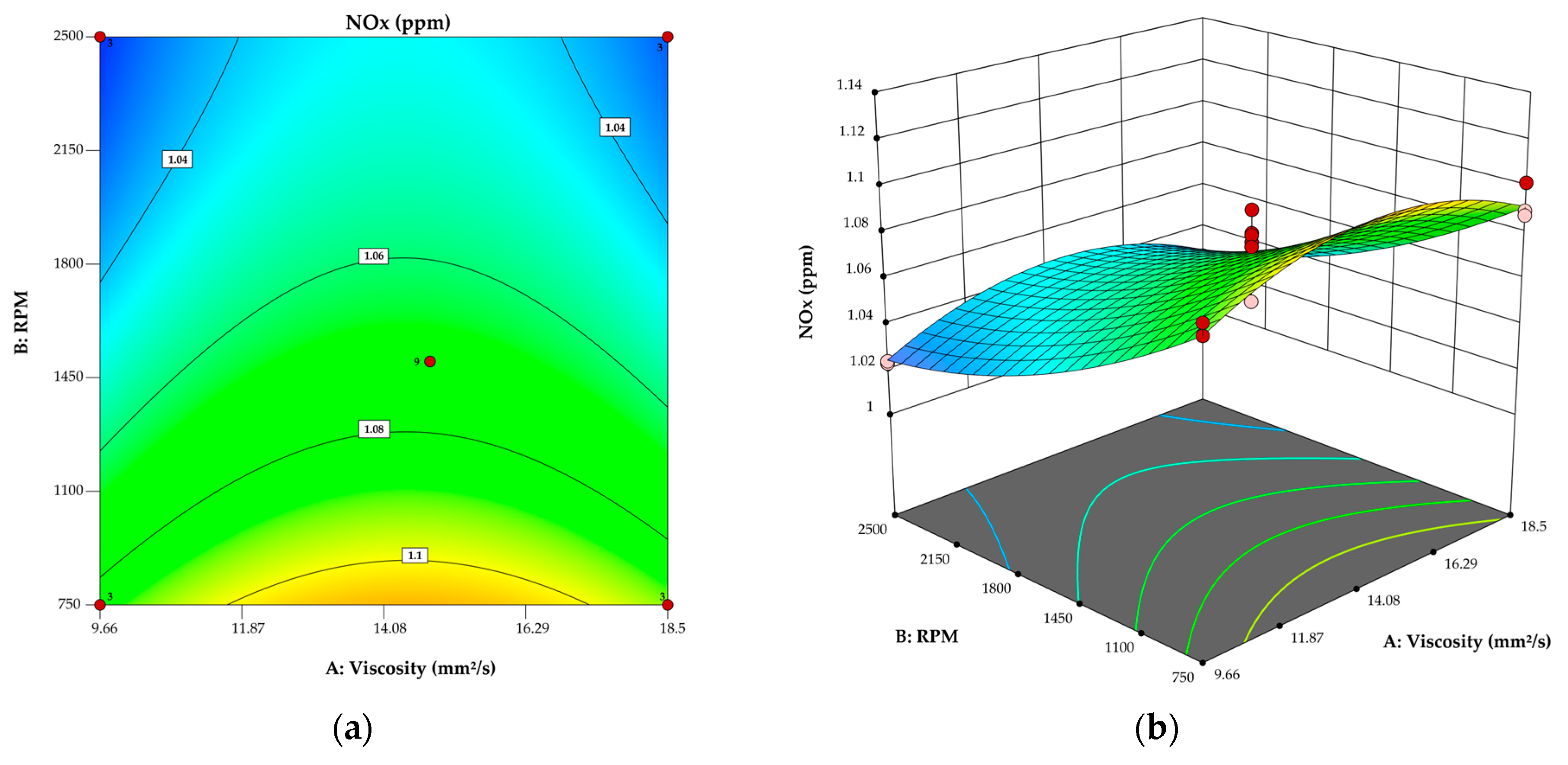
3.3. Model for NOx
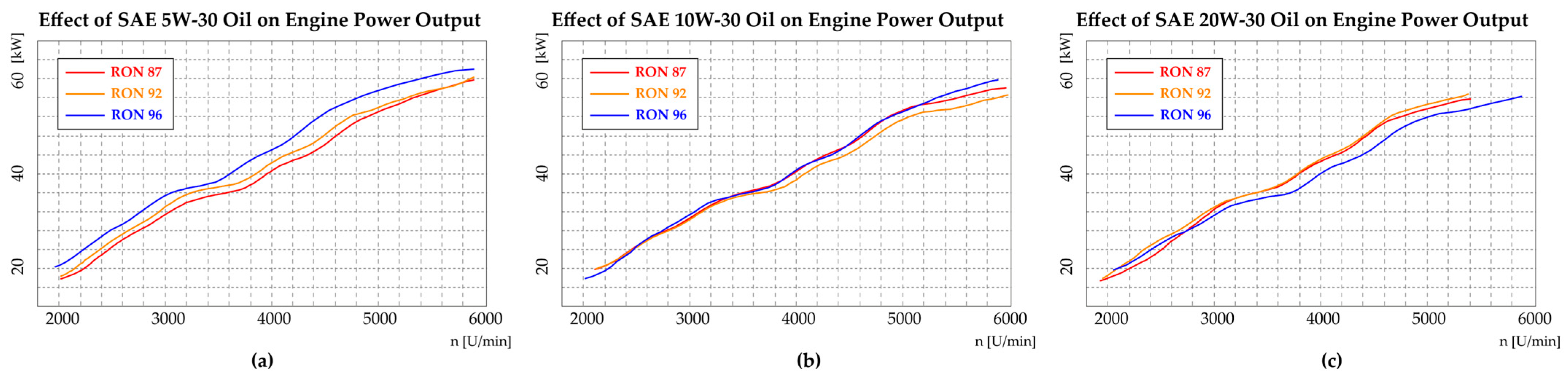
3.4. Analysis of Effect of Oil Viscosity on Engine Performance
4. Discussion
5. Conclusions
Author Contributions
Funding
Data Availability Statement
Conflicts of Interest
References
- Rodríguez-Fernández, J.; Ramos, Á.; Barba, J.; Cárdenas, D.; Delgado, J. Improving Fuel Economy and Engine Performance through Gasoline Fuel Octane Rating. Energies 2020, 13, 3499. [Google Scholar] [CrossRef]
- Fernanda, M.A.; Irawan, B. Effect of Different Octane Number on Power and Specific Fuel Consumption in Gasoline Compression Ignition Engine. Evrimata J. Mech. Eng. 2024. [Google Scholar] [CrossRef]
- Sayin, C. The Impact of Varying Spark Timing at Different Octane Numbers on the Performance and Emission Characteristics in a Gasoline Engine. Fuel 2012, 97, 856–861. [Google Scholar] [CrossRef]
- Sayin, C.; Kilicaslan, I.; Canakci, M.; Ozsezen, N. An Experimental Study of the Effect of Octane Number Higher than Engine Requirement on the Engine Performance and Emissions. Appl. Therm. Eng. 2005, 25, 1315–1324. [Google Scholar] [CrossRef]
- Athafah, N.; Salih, A. Effect of Octane Number on Performance and Exhaust Emissions of an SI Engine. Eng. Technol. J. 2020, 38, 574–585. [Google Scholar] [CrossRef]
- Al-Farayedhi, A.A. Effects of Octane Number on Exhaust Emissions of a Spark Ignition Engine. Int. J. Energy Res. 2002, 26, 279–289. [Google Scholar] [CrossRef]
- Iodice, P.; Amoresano, A.; Langella, G. A Review on the Effects of Ethanol/Gasoline Fuel Blends on NOX Emissions in Spark-Ignition Engines. Biofuel Res. J. 2021, 8, 1465–1480. [Google Scholar] [CrossRef]
- Khalifa, A.E.; Antar, M.A.; Farag, M.S. Experimental and Theoretical Comparative Study of Performance and Emissions for a Fuel Injection SI Engine with Two Octane Blends. Arab. J. Sci. Eng. 2015, 40, 1743–1756. [Google Scholar] [CrossRef]
- Zhang, Y.; Ma, Z.; Feng, Y.; Diao, Z.; Liu, Z. The Effects of Ultra-Low Viscosity Engine Oil on Mechanical Efficiency and Fuel Economy. Energies 2021, 14, 2320. [Google Scholar] [CrossRef]
- Hei, D.; Zheng, M.; Liu, C.; Jiang, L.; Zhang, Y.; Zhao, X. Study on the Frictional Properties of the Top Ring-Liner Conjunction for Different-Viscosity Lubricant. Adv. Mech. Eng. 2023, 15, 16878132231155002. [Google Scholar] [CrossRef]
- Mu, J.; Wu, J.; Han, F.; Li, J.; Su, L. Effect of Non-Functional Additives on Performance of Internal Combustion Engine Lubricating Oil; Springer: Berlin/Heidelberg, Germany, 2018; pp. 691–698. [Google Scholar]
- Palikhel, L.; Karn, R.L.; Aryal, S.; Neupane, B. Effect of Natural and Synthesized Oil Blends with Diesel by Volume on Lubrication and Performance of Internal Combustion Engine. J. Innov. Eng. Educ. 2020, 3, 107–114. [Google Scholar] [CrossRef]
- Giakoumis, E.G. Lubricating Oil Effects on the Transient Performance of a Turbocharged Diesel Engine. Energy 2010, 35, 864–873. [Google Scholar] [CrossRef]
- Santana, C. Correlation Between Vibration Level, Lubricating Oil Viscosity and Total Number Base of an Internal Combustion Engine Operated with Gasoline and Ethanol; SAE Technical Paper; SAE International: Warrendale, PA, USA, 2022. [Google Scholar] [CrossRef]
- Ayele, Y.; Stuecken, T.; Schock, H. A Study of the Influence of Orifice Diameter on a Dual Mode, Turbulent Jet Ignition Engine through Variable Engine Speed. Int. J. Engine Res. 2023, 24, 1704–1713. [Google Scholar] [CrossRef]
- Song, J.; Song, H.H. Spark-Ignition Engine Speed Profile Optimization for Maximizing the Net Indicated Efficiency and Quantitative Analysis of the Optimal Speed Profile. Appl. Energy 2022, 307, 118162. [Google Scholar] [CrossRef]
- Olaiya, K.A.; Alabi, I.O.; Okediji, A.P. Performance Characteristics of a Single-Cylinder Two-Stroke Diesel Engine Using Diesel-RK Software. Int. J. Sci. Eng. Res. 2020, 11, 463–472. [Google Scholar]
- Shinde, B.J.; Karunamurthy, K.; Ismail, S. Thermodynamic Analysis of Gasoline-Fueled Electronic Fuel Injection Digital Three-Spark Ignition (EFI-DTSI) Engine. J. Therm. Anal. Calorim. 2020, 141, 2355–2367. [Google Scholar] [CrossRef]
- Wang, K.; Zhang, Z.; Sun, B.; Zhang, S.; Lai, F.; Ma, N.; Ju, X.; Luo, Q.; Bao, L.-Z. Experimental Investigation of the Working Boundary Limited by Abnormal Combustion and the Combustion Characteristics of a Turbocharged Direct Injection Hydrogen Engine. Energy Convers. Manag. 2024, 299, 117861. [Google Scholar] [CrossRef]
- Ghaderi Masouleh, M.; Keskinen, K.; Kaario, O.; Kahila, H.; Karimkashi, S.; Vuorinen, V. Modeling Cycle-to-Cycle Variations in Spark Ignited Combustion Engines by Scale-Resolving Simulations for Different Engine Speeds. Appl. Energy 2019, 250, 801–820. [Google Scholar] [CrossRef]
- Gao, J.; Tian, G.; Jenner, P.; Burgess, M. Intake Characteristics and Pumping Loss in the Intake Stroke of a Novel Small Scale Opposed Rotary Piston Engine. J. Clean. Prod. 2020, 261, 121180. [Google Scholar] [CrossRef]
- Ijaz Malik, M.A.; Usman, M.; Akhtar, M.; Farooq, M.; Saleem Iqbal, H.M.; Irshad, M.; Shah, M.H. Response Surface Methodology Application on Lubricant Oil Degradation, Performance, and Emissions in SI Engine: A Novel Optimization of Alcoholic Fuel Blends. Sci. Prog. 2023, 106, 368504221148342. [Google Scholar] [CrossRef]
- Safieddin Ardebili, S.M.; Solmaz, H.; Calam, A.; İpci, D. Modelling of Performance, Emission, and Combustion of an HCCI Engine Fueled with Fusel Oil-Diethylether Fuel Blends as a Renewable Fuel. Fuel 2021, 290, 120017. [Google Scholar] [CrossRef]
- Katekaew, S.; Suiuay, C.; Senawong, K.; Seithtanabutara, V.; Intravised, K.; Laloon, K. Optimization of Performance and Exhaust Emissions of Single-Cylinder Diesel Engines Fueled by Blending Diesel-like Fuel from Yang-Hard Resin with Waste Cooking Oil Biodiesel via Response Surface Methodology. Fuel 2021, 304, 121434. [Google Scholar] [CrossRef]
- Liang, X.; Zhao, B.; Wang, K.; Wang, Y.; Wang, Y.; Lv, X. Application of Response Surface Methodology for the Joint Optimization of Performance and Emission Characteristics of a Diesel Engine. Int. J. Green Energy 2021, 18, 697–707. [Google Scholar] [CrossRef]
- Kumar, M.; Gautam, R.; Ansari, N.A. Performance Characteristics Optimization of CRDI Engine Fuelled with a Blend of Sesame Oil Methyl Ester and Diesel Fuel Using Response Surface Methodology Approach. Front. Mech. Eng. 2023, 9, 1049571. [Google Scholar] [CrossRef]
- NTE INEN 935; (11ª Edición): Productos Derivados de Petróleo. Gasolina. Requisitos; Resolución MPCEIP-SC-2021-0137-R; Registro Oficial No. 541, 20 de Septiembre de 2021. INEN: Quito, Ecuador, 2021.
- Awad, O.I.; Mamat, R.; Ali, O.M.; Azmi, W.H.; Kadirgama, K.; Yusri, I.M.; Leman, A.M.; Yusaf, T. Response Surface Methodology (RSM) Based Multi-Objective Optimization of Fusel Oil -Gasoline Blends at Different Water Content in SI Engine. Energy Convers. Manag. 2017, 150, 222–241. [Google Scholar] [CrossRef]
- Yusri, I.M.; Mamat, R.; Azmi, W.H.; Omar, A.I.; Obed, M.A.; Shaiful, A.I.M. Application of Response Surface Methodology in Optimization of Performance and Exhaust Emissions of Secondary Butyl Alcohol-Gasoline Blends in SI Engine. Energy Convers. Manag. 2017, 133, 178–195. [Google Scholar] [CrossRef]

| Author(s) | Engine Type | Variables Studied | Methodology |
|---|---|---|---|
| Zhang et al. [9] | Gasoline engine | Oil viscosity (0W-16 vs. 5W-30) | Experimental evaluation of fuel economy and wear |
| Fernanda et al. [2] | Spark ignition engine | Octane rating effect | Performance tests and measurement of fuel consumption |
| Sayın et al. [4] | Gasoline engine (non-optimized) | High-octane fuel in standard engine | Comparative fuel analysis |
| Iodice et al. [7] | Spark ignition engine | Octane rating and NOx formation | Combustion analysis |
| Giakoumis [13] | Turbocharged diesel engine | High-viscosity oil and transient operation | Simulation and empirical data |
| Khalifa et al. [8] | Engine without knock control | Octane rating and THC emissions | Experimental tests |
| Technical Specifications | |
|---|---|
| Engine | 2.0 L SOHC |
| Valves | 16 |
| Number of cylinders | 4 |
| Power (CV @ rpm) | 140 @ 5600 |
| Torque (Nm @ rpm) | 183 @ 4000 |
| Fuel supply | Multi-point fuel injection (MPFI) |
| Compression ratio | 10.5:1 |
| Final ratio | 3.944 |
| Gross vehicle weight | 1608 Kg |
| Measuring Fields | Range | Unit | Resolution |
|---|---|---|---|
| CO | 0–9.99 | % vol | 0.01 |
| CO2 | 0–19.9 | % vol | 0.1 |
| HC hexane | 0–9999 | ppm vol | 1 |
| O2 | 0–25 | % vol | 0.01 |
| NOx | 0–5000 | ppm vol | 1 |
| Revolution inductance/capacitance | 300–9990 | rpm | 10 |
| Oil temperature | 20–150 | °C | 1 |
| SAE Grade | 5W30 | 10W30 | 20W50 |
|---|---|---|---|
| Specific gravity @ 15 °C | 0.861 | 0.866 | 0.881 |
| Density, g/mL @ 15 °C | 0.859 | 0.864 | 0.878 |
| Color, ASTM D1500 | 3.0 | 3.0 | 3.0 |
| Flash point (COC), °C (°F) | 216 (421) | 229 (444) | 230 (446) |
| Pour point, °C (°F) | −39 (−38) | −39 (−38) | −30 (−22) |
| Kinematic viscosity, mm2/s @ 40 °C | 66.2 | 65.7 | 176 |
| Kinematic viscosity, mm2/s @ 100 °C | 9.66 | 14.08 | 18.5 |
| Viscosity index | 158 | 148 | 128 |
| Cold cranking viscosity, cP @ (°C) | 6150 (−30) | 4550 (−25) | 7200 (−15) |
| High-temp/high-shear viscosity, cP @ 150 °C | 3.1 | 3.0 | 4.9 |
| Requirements | Ecopaís Gasoline | Super Gasoline |
|---|---|---|
| Research octane number (RON) | 87 | 92 |
| Vapor pressure [kPa] | 60 | 60 |
| Distillation residue [%] | 2 max | 2 max |
| Gum content [mg/100 mL] | 3 max | 4 mx |
| Sulfur content [%] | 0.065 max | 0.065 max |
| Aromatics content [%] | 30 max | 30 max |
| Benzene content [%] | 1 max | 2 mx |
| Olefin content [%] | 18 max | 25 max |
| Oxygen content [% | 2.7 max | 2.7 max |
| Pb content [mg/L] | Not detectable | Not detectable |
| Manganese content [mg/L] | Not detectable | Not detectable |
| Iron content [mg/L] | Not detectable | Not detectable |
| Factor | Unit | Lower Level | Middle Level | Upper Level |
|---|---|---|---|---|
| Viscosity | mm2/s | 9.66 | 14.8 | 18.5 |
| Fuel quality | Research octane number (RON) | −1 | 0 | 1 |
| Engine speed | rpm | 750 | 1500 | 2500 |
| Std Order | Run Order | Pt Type | Blocks | Viscosity (mm2/s) | rpm | Fuel (RON) | CO2 (% vol) | HC (ppm) | NOx (ppm) |
|---|---|---|---|---|---|---|---|---|---|
| 30 | 1 | 0 | 2 | 14.8 | 1500 | 0 | 13.7 | 23 | 1.09 |
| 18 | 2 | 2 | 2 | 9.66 | 2500 | 0 | 14.4 | 1 | 1.023 |
| 16 | 3 | 2 | 2 | 9.66 | 750 | 0 | 13.5 | 1 | 1.09 |
| 26 | 4 | 2 | 2 | 14.8 | 750 | 1 | 12.9 | 30 | 1.127 |
| 23 | 5 | 2 | 2 | 18.5 | 1500 | 1 | 14.2 | 9 | 1.054 |
| 21 | 6 | 2 | 2 | 18.5 | 1500 | −1 | 14.2 | 11 | 1.057 |
| 29 | 7 | 0 | 2 | 14.8 | 1500 | 0 | 14.2 | 33 | 1.07 |
| 27 | 8 | 2 | 2 | 14.8 | 2500 | 1 | 14 | 22 | 1.032 |
| 22 | 9 | 2 | 2 | 9.66 | 1500 | 1 | 14.2 | 8 | 1.05 |
| 25 | 10 | 2 | 2 | 14.8 | 2500 | −1 | 13.9 | 10 | 1.05 |
| 24 | 11 | 2 | 2 | 14.8 | 750 | −1 | 13.6 | 12 | 1.09 |
| 20 | 12 | 2 | 2 | 9.66 | 1500 | −1 | 14.1 | 26 | 1.042 |
| 19 | 13 | 2 | 2 | 18.5 | 2500 | 0 | 14.5 | 1 | 1.024 |
| 28 | 14 | 0 | 2 | 14.8 | 1500 | 0 | 13.9 | 32 | 1.08 |
| 17 | 15 | 2 | 2 | 18.5 | 750 | 0 | 13.5 | 1 | 1.102 |
| 12 | 16 | 2 | 1 | 14.8 | 2500 | 1 | 14.3 | 23 | 1.019 |
| 15 | 17 | 0 | 1 | 14.8 | 1500 | 0 | 13.9 | 23 | 1.076 |
| 8 | 18 | 2 | 1 | 18.5 | 1500 | 1 | 14.4 | 9 | 1.051 |
| 13 | 19 | 0 | 1 | 14.8 | 1500 | 0 | 13.9 | 23 | 1.079 |
| 14 | 20 | 0 | 1 | 14.8 | 1500 | 0 | 14.2 | 21 | 1.05 |
| 10 | 21 | 2 | 1 | 14.8 | 2500 | −1 | 13.9 | 10 | 1.07 |
| 11 | 22 | 2 | 1 | 14.8 | 750 | 1 | 13.1 | 31 | 1.113 |
| 4 | 23 | 2 | 1 | 18.5 | 2500 | 0 | 14.5 | 2 | 1.025 |
| 3 | 24 | 2 | 1 | 9.66 | 2500 | 0 | 14.4 | 1 | 1.024 |
| 9 | 25 | 2 | 1 | 14.8 | 750 | −1 | 13 | 13 | 1.1 |
| 6 | 26 | 2 | 1 | 18.5 | 1500 | −1 | 14.2 | 10 | 1.044 |
| 2 | 27 | 2 | 1 | 18.5 | 750 | 0 | 13.6 | 2 | 1.088 |
| 7 | 28 | 2 | 1 | 9.66 | 1500 | 1 | 14.3 | 8 | 1.046 |
| 5 | 29 | 2 | 1 | 9.66 | 1500 | −1 | 14.1 | 25 | 1.04 |
| 1 | 30 | 2 | 1 | 9.66 | 750 | 0 | 13.5 | 1 | 1.09 |
| 41 | 31 | 2 | 3 | 14.8 | 750 | 1 | 13.3 | 31 | 1.104 |
| 35 | 32 | 2 | 3 | 9.66 | 1500 | −1 | 14.2 | 26 | 1.038 |
| 32 | 33 | 2 | 3 | 18.5 | 750 | 0 | 13.6 | 1 | 1.09 |
| 37 | 34 | 2 | 3 | 9.66 | 1500 | 1 | 14.3 | 7 | 1.05 |
| 39 | 35 | 2 | 3 | 14.8 | 750 | −1 | 13.5 | 13 | 1.08 |
| 36 | 36 | 2 | 3 | 18.5 | 1500 | −1 | 14.2 | 11 | 1.045 |
| 45 | 37 | 0 | 3 | 14.8 | 1500 | 0 | 14.2 | 22 | 1.068 |
| 33 | 38 | 2 | 3 | 9.66 | 2500 | 0 | 14.4 | 1 | 1.023 |
| 38 | 39 | 2 | 3 | 18.5 | 1500 | 1 | 14.3 | 8 | 1.063 |
| 42 | 40 | 2 | 3 | 14.8 | 2500 | 1 | 14.3 | 22 | 1.023 |
| 43 | 41 | 0 | 3 | 14.8 | 1500 | 0 | 14.2 | 32 | 1.05 |
| 44 | 42 | 0 | 3 | 14.8 | 1500 | 0 | 14 | 33 | 1.074 |
| 34 | 43 | 2 | 3 | 18.5 | 2500 | 0 | 14.3 | 2 | 1.026 |
| 40 | 44 | 2 | 3 | 14.8 | 2500 | −1 | 13.5 | 11 | 1.08 |
| 31 | 45 | 2 | 3 | 9.66 | 750 | 0 | 13.6 | 2 | 1.085 |
| Source | Sum of Squares | Df | Mean Square | F-Value | p-Value | |
|---|---|---|---|---|---|---|
| Model | 6.72 | 9 | 0.7465 | 31.40 | <0.0001 | Significant |
| A—Viscosity | 0.0099 | 1 | 0.0099 | 0.4183 | 0.5220 | |
| B—RPM | 3.88 | 1 | 3.88 | 163.11 | <0.0001 | |
| C—Fuel | 0.0938 | 1 | 0.0938 | 3.94 | 0.0549 | |
| AB | 0.0003 | 1 | 0.0003 | 0.0141 | 0.9062 | |
| AC | 0.0016 | 1 | 0.0016 | 0.0681 | 0.7956 | |
| BC | 0.3594 | 1 | 0.3594 | 15.11 | 0.0004 | |
| A2 | 0.9348 | 1 | 0.9348 | 39.31 | <0.0001 | |
| B2 | 1.63 | 1 | 1.63 | 68.59 | <0.0001 | |
| C2 | 0.0820 | 1 | 0.0820 | 3.45 | 0.0717 | |
| Residual | 0.8322 | 35 | 0.0238 | |||
| Lack of fit | 0.0300 | 3 | 0.0100 | 0.3992 | 0.7545 | Not significant |
| Pure error | 0.8022 | 32 | 0.0251 | |||
| Cor total | 7.55 | 44 |
| Coefficient of Determination | Value |
|---|---|
| R2 | 0.8898 |
| Adjusted R2 | 0.8614 |
| Predicted R2 | 0.8236 |
| Adeq Precision | 18.0130 |
| Source | Sum of Squares | Df | Mean Square | F-Value | p-Value | |
|---|---|---|---|---|---|---|
| Model | 4175.25 | 9 | 463.92 | 13.37 | <0.0001 | |
| A—Viscosity | 64.85 | 1 | 64.85 | 1.87 | 0.1803 | |
| B—RPM | 43.19 | 1 | 43.19 | 1.24 | 0.2722 | |
| C—Fuel | 14.97 | 1 | 14.97 | 0.4315 | 0.5156 | |
| AB | 0.5239 | 1 | 0.5239 | 0.0151 | 0.9029 | |
| AC | 299.09 | 1 | 299.09 | 8.62 | 0.0058 | |
| BC | 5.25 | 1 | 5.25 | 0.1513 | 0.6996 | |
| A2 | 2789.47 | 1 | 2789.47 | 80.40 | <0.0001 | |
| B2 | 1026.26 | 1 | 1026.26 | 29.58 | <0.0001 | |
| C2 | 42.98 | 1 | 42.98 | 1.24 | 0.2733 | |
| Residual | 1214.40 | 35 | 34.70 | |||
| Lack of fit | 976.17 | 3 | 325.39 | 43.71 | <0.0001 | Significant |
| Pure error | 238.22 | 32 | 7.44 | |||
| Cor total | 5389.64 | 44 |
| Coefficient of Determination | Value |
|---|---|
| R2 | 0.7747 |
| Adjusted R2 | 0.7167 |
| Predicted R2 | 0.6237 |
| Adeq Precision | 10.2101 |
| Source | Sum of Squares | Df | Mean Square | F-Value | p-Value | |
|---|---|---|---|---|---|---|
| Model | 0.0315 | 9 | 0.0035 | 38.46 | <0.0001 | Significant |
| A—Viscosity | 0.0002 | 1 | 0.0002 | 2.04 | 0.1623 | |
| B—RPM | 0.0225 | 1 | 0.0225 | 247.02 | <0.0001 | |
| C—Fuel | 0.0000 | 1 | 0.0000 | 0.4503 | 0.5066 | |
| AB | 4.12 × 10⁻⁶ | 1 | 4.12 × 10⁻⁶ | 0.0453 | 0.8327 | |
| AC | 7.83 × 10⁻⁶ | 1 | 7.83 × 10⁻⁶ | 0.0862 | 0.7708 | |
| BC | 0.0035 | 1 | 0.0035 | 38.89 | <0.0001 | |
| A2 | 0.0040 | 1 | 0.0040 | 43.50 | <0.0001 | |
| B2 | 0.0012 | 1 | 0.0012 | 13.56 | 0.0008 | |
| C2 | 0.0001 | 1 | 0.0001 | 1.07 | 0.3077 | |
| Residual | 0.0032 | 35 | 0.0001 | |||
| Lack of Fit | 0.0004 | 3 | 0.0001 | 1.49 | 0.2349 | Not significant |
| Pure Error | 0.0028 | 32 | 0.0001 | |||
| Cor Total | 0.0346 | 44 |
| Coefficient of Determination | Value |
|---|---|
| R2 | 0.9082 |
| Adjusted R2 | 0.8846 |
| Predicted R2 | 0.8584 |
| Adeq Precision | 21.3603 |
| Oil | RON | Power [kW] |
|---|---|---|
| 5W30 | 87 | 59.5 |
| 92 | 58.8 | |
| 95 | 60.2 | |
| 10W30 | 87 | 57.9 |
| 92 | 56.3 | |
| 95 | 59.5 | |
| 20W50 | 87 | 55.6 |
| 92 | 56.5 | |
| 95 | 55.9 |
Disclaimer/Publisher’s Note: The statements, opinions and data contained in all publications are solely those of the individual author(s) and contributor(s) and not of MDPI and/or the editor(s). MDPI and/or the editor(s) disclaim responsibility for any injury to people or property resulting from any ideas, methods, instructions or products referred to in the content. |
© 2025 by the authors. Licensee MDPI, Basel, Switzerland. This article is an open access article distributed under the terms and conditions of the Creative Commons Attribution (CC BY) license (https://creativecommons.org/licenses/by/4.0/).
Share and Cite
Garcia Tobar, M.; Pinta Pesantez, K.; Jimenez Romero, P.; Contreras Urgiles, R.W. The Impact of Oil Viscosity and Fuel Quality on Internal Combustion Engine Performance and Emissions: An Experimental Approach. Lubricants 2025, 13, 188. https://doi.org/10.3390/lubricants13040188
Garcia Tobar M, Pinta Pesantez K, Jimenez Romero P, Contreras Urgiles RW. The Impact of Oil Viscosity and Fuel Quality on Internal Combustion Engine Performance and Emissions: An Experimental Approach. Lubricants. 2025; 13(4):188. https://doi.org/10.3390/lubricants13040188
Chicago/Turabian StyleGarcia Tobar, Milton, Kevin Pinta Pesantez, Pablo Jimenez Romero, and Rafael Wilmer Contreras Urgiles. 2025. "The Impact of Oil Viscosity and Fuel Quality on Internal Combustion Engine Performance and Emissions: An Experimental Approach" Lubricants 13, no. 4: 188. https://doi.org/10.3390/lubricants13040188
APA StyleGarcia Tobar, M., Pinta Pesantez, K., Jimenez Romero, P., & Contreras Urgiles, R. W. (2025). The Impact of Oil Viscosity and Fuel Quality on Internal Combustion Engine Performance and Emissions: An Experimental Approach. Lubricants, 13(4), 188. https://doi.org/10.3390/lubricants13040188