
Bioacoustic IoT Sensors as Next-Generation Tools for Monitoring: Counting Flying Insects through Buzz
 , , and
Abstract
:Simple Summary
Abstract

1. Introduction
2. Materials and Methods
2.1. Study Areas
- Site A→located in northern Italy in the municipality of Grezzana (VR), Veneto (45.516667°, 11.016667°); a very diversified farm of about 40 ha, with land mainly used for wine production, smaller areas of olive groves, and deciduous woodland. Annual temperatures range from −7 °C to 37 °C (9–32 °C between mid-April and mid-June 2023), and monthly precipitation between 30 mm and 77 mm (58–62 mm between mid-April and mid-June 2023).
- Site B→located in central-northern Italy in the municipality of Medicina (BO), Emilia-Romagna (44.483333°, 11.633333°); 30 ha of arable crops surrounded by similar agricultural landscape. Annual temperatures range from −5 °C to 38 °C (7–34 °C between mid-April and mid-June 2023), and monthly precipitation between 27 mm and 66 mm (40–46 mm between mid-April and mid-June 2023).
- Site C→located in central Italy in the municipality of Viterbo (VT), Lazio (42.418611°, 12.104167°); an area of approximately 2 ha used for growing hazelnuts (Corylus avellana), surrounded by a dirt road with spontaneous aromatic flowers and other hazelnut groves. Annual temperatures range from −1 °C to 37 °C (8–29 °C between mid-April and mid-June 2023), and monthly precipitation between 18 mm and 86 mm (30–45 mm between mid-April and mid-June 2023).
- Site D→located in central Italy in the municipality of Viterbo (VT), Lazio (42.421027°, 12.129143°); an area of approximately 1 ha where half is used for the cultivation of hazelnuts (Corylus avellana) while the other half has been left to spontaneous re-naturalisation; it is set in a broadleaf woodland context (chestnut and beech woods). Annual temperatures range from −1 °C to 37 °C (8–29 °C between mid-April and mid-June 2023), and monthly precipitation between 18 mm and 86 mm (30–45 mm between mid-April and mid-June 2023).
2.2. Spectrum
- Fourier Transformation: The captured signal undergoes Fourier Transformation at a resolution of 5 Hz, converting it from the time domain to the frequency domain;
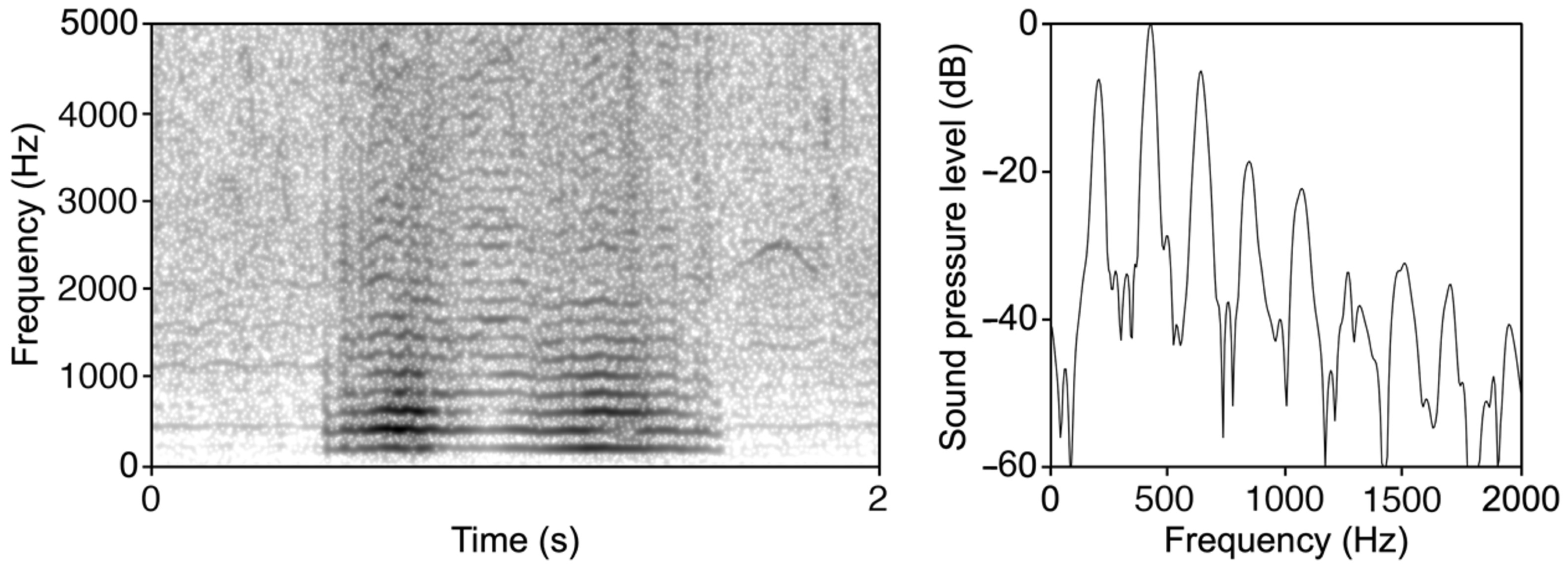
- Buzz Pattern Identification: The transformed data are then processed by an algorithm to identify and enumerate patterns classifiable as ‘buzz’. The algorithm detects the fundamental frequency and checks for subsequent peaks at higher harmonics (see Figure 1).
2.3. Invertebrate Surveys: Traditional Methods
2.4. Statistical Analysis
3. Results
3.1. Data Analysis
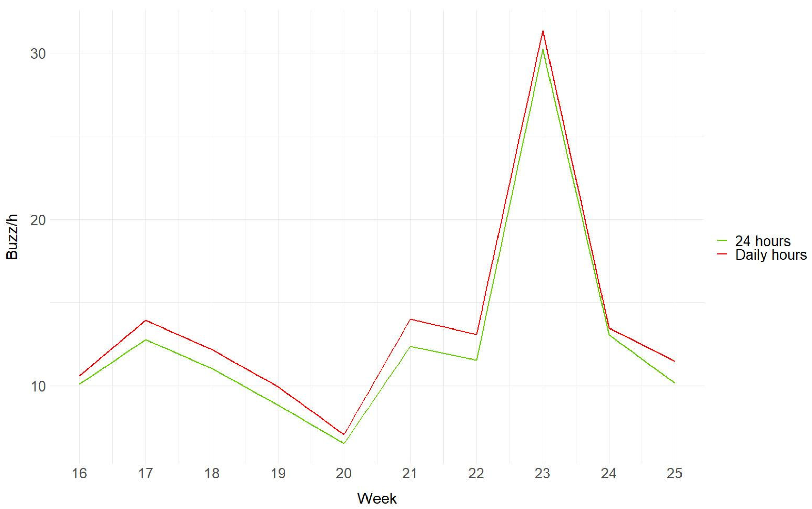
3.2. Hourly and Weekly Variation of Buzzes
4. Discussion
5. Conclusions
Author Contributions
Funding
Data Availability Statement
Conflicts of Interest
References
- Almond, R.E.A.; Grooten, M.; Juffe Bignoli, D.; Petersen, T. Living Planet Report 2022—Building a Nature Positive Society; WWF: Gland, Switzerland, 2022. [Google Scholar]
- Pascual, U.; Adams, W.M.; Díaz, S.; Lele, S.; Mace, G.M.; Turnhout, E. Biodiversity and the Challenge of Pluralism. Nat. Sustain. 2021, 4, 567–572. [Google Scholar] [CrossRef]
- Butchart, S.H.M.; Walpole, M.; Collen, B.; van Strien, A.; Scharlemann, J.P.W.; Almond, R.E.A.; Baillie, J.E.M.; Bomhard, B.; Brown, C.; Bruno, J.; et al. Global Biodiversity: Indicators of Recent Declines. Science 2010, 328, 1164–1168. [Google Scholar] [CrossRef] [PubMed]
- Scanes, C.G. Chapter 19—Human Activity and Habitat Loss: Destruction, Fragmentation, and Degradation. In Animals and Human Society; Scanes, C.G., Toukhsati, S.R., Eds.; Academic Press: Cambridge, MA, USA, 2018; pp. 451–482. ISBN 978-0-12-805247-1. [Google Scholar]
- Prakash, S.; Verma, A.K. Anthropogenic Activities and Biodiversity Threats. Int. J. Biol. Innov. 2022, 4, 94–103. [Google Scholar] [CrossRef]
- Díaz, S.; Settele, J.; Brondízio, E.S.; Ngo, H.T.; Agard, J.; Arneth, A.; Balvanera, P.; Brauman, K.A.; Butchart, S.H.M.; Chan, K.M.A.; et al. Pervasive Human-Driven Decline of Life on Earth Points to the Need for Transformative Change. Science 2019, 366, eaax3100. [Google Scholar] [CrossRef] [PubMed]
- Landmann, T.; Schmitt, M.; Ekim, B.; Villinger, J.; Ashiono, F.; Habel, J.C.; Tonnang, H.E.Z. Insect Diversity Is a Good Indicator of Biodiversity Status in Africa. Commun. Earth Environ. 2023, 4, 234. [Google Scholar] [CrossRef]
- Choudhary, A.; Ahi, J. Biodiversity of Freshwater Insects: A Review. Int. J. Eng. Sci. 2015, 4, 25–31. [Google Scholar]
- Conrad, K.F.; Fox, R.; Woiwod, I.P. Monitoring Biodiversity: Measuring Long-Term Changes in Insect Abundance. In Insect Conservation Biology; CABI: Wallingford, UK, 2007; pp. 203–225. [Google Scholar]
- Food and Agriculture Organization (FAO). Tools for Conservation and Use of Pollination Services—Initial Survey of Good Pollination Practices; Food and Agriculture Organization (FAO): Rome, Italy, 2008. [Google Scholar]
- Decourtye, A.; Alaux, C.; Le Conte, Y.; Henry, M. Toward the Protection of Bees and Pollination under Global Change: Present and Future Perspectives in a Challenging Applied Science. Curr. Opin. Insect Sci. 2019, 35, 123–131. [Google Scholar] [CrossRef]
- Patel, V.; Pauli, N.; Biggs, E.; Barbour, L.; Boruff, B. Why Bees Are Critical for Achieving Sustainable Development. Ambio 2021, 50, 49–59. [Google Scholar] [CrossRef]
- Brown, K.S., Jr.; Freitas, A.V.L. Atlantic Forest Butterflies: Indicators for Landscape Conservation1. Biotropica 2000, 32, 934–956. [Google Scholar] [CrossRef]
- Scudder, G.G.E. The Importance of Insects. In Insect Biodiversity; John Wiley & Sons, Ltd.: Hoboken, NJ, USA, 2017; pp. 9–43. ISBN 978-1-118-94556-8. [Google Scholar]
- Hallmann, C.A.; Sorg, M.; Jongejans, E.; Siepel, H.; Hofland, N.; Schwan, H.; Stenmans, W.; Müller, A.; Sumser, H.; Hörren, T.; et al. More than 75 Percent Decline over 27 Years in Total Flying Insect Biomass in Protected Areas. PLoS ONE 2017, 12, e0185809. [Google Scholar] [CrossRef]
- Martin, A.E.; Graham, S.L.; Henry, M.; Pervin, E.; Fahrig, L. Flying Insect Abundance Declines with Increasing Road Traffic. Insect Conserv. Divers. 2018, 11, 608–613. [Google Scholar] [CrossRef]
- Cooley, J.R. Floral Heat Rewards and Direct Benefits to Insect Pollinators. Ann. Entomol. Soc. Am. 1995, 88, 576–579. [Google Scholar] [CrossRef]
- Didham, R.K.; Barbero, F.; Collins, C.M.; Forister, M.L.; Hassall, C.; Leather, S.R.; Packer, L.; Saunders, M.E.; Stewart, A.J.A. Spotlight on Insects: Trends, Threats and Conservation Challenges. Insect Conserv. Divers. 2020, 13, 99–102. [Google Scholar] [CrossRef]
- Lövei, G.L.; Ferrante, M. The Use and Prospects of Nonlethal Methods in Entomology. Annu. Rev. Entomol. 2024, 69, 183–198. [Google Scholar] [CrossRef] [PubMed]
- McCravy, K.W. A Review of Sampling and Monitoring Methods for Beneficial Arthropods in Agroecosystems. Insects 2018, 9, 170. [Google Scholar] [CrossRef]
- O’Connor, R.S.; Kunin, W.E.; Garratt, M.P.; Potts, S.G.; Roy, H.E.; Andrews, C.; Jones, C.M.; Peyton, J.M.; Savage, J.; Harvey, M.C.; et al. Monitoring Insect Pollinators and Flower Visitation: The Effectiveness and Feasibility of Different Survey Methods. Methods Ecol. Evol. 2019, 10, 2129–2140. [Google Scholar] [CrossRef]
- Ma, C.-S.; Ma, G.; Pincebourde, S. Survive a Warming Climate: Insect Responses to Extreme High Temperatures. Annu. Rev. Entomol. 2021, 66, 163–184. [Google Scholar] [CrossRef]
- Ma, G.; Hoffmann, A.A.; Ma, C.-S. Daily Temperature Extremes Play an Important Role in Predicting Thermal Effects. J. Exp. Biol. 2015, 218, 2289–2296. [Google Scholar] [CrossRef]
- Paaijmans, K.P.; Heinig, R.L.; Seliga, R.A.; Blanford, J.I.; Blanford, S.; Murdock, C.C.; Thomas, M.B. Temperature Variation Makes Ectotherms More Sensitive to Climate Change. Glob. Chang. Biol. 2013, 19, 2373–2380. [Google Scholar] [CrossRef]
- Easterling, D.R.; Meehl, G.A.; Parmesan, C.; Changnon, S.A.; Karl, T.R.; Mearns, L.O. Climate Extremes: Observations, Modeling, and Impacts. Science 2000, 289, 2068–2074. [Google Scholar] [CrossRef]
- Cormont, A.; Malinowska, A.H.; Kostenko, O.; Radchuk, V.; Hemerik, L.; WallisDeVries, M.F.; Verboom, J. Effect of Local Weather on Butterfly Flight Behaviour, Movement, and Colonization: Significance for Dispersal under Climate Change. Biodivers. Conserv. 2011, 20, 483–503. [Google Scholar] [CrossRef]
- Corbet, S.A.; Fussell, M.; Ake, R.; Fraser, A.; Gunson, C.; Savage, A.; Smith, K. Temperature and the Pollinating Activity of Social Bees. Ecol. Entomol. 1993, 18, 17–30. [Google Scholar] [CrossRef]
- Kwon, Y.J.; Saeed, S. Effect of Temperature on the Foraging Activity of Bombus terrestris L. (Hymenoptera: Apidae) on Greenhouse Hot Pepper (Capsicum annuum L.). Appl. Entomol. Zool. 2003, 38, 275–280. [Google Scholar] [CrossRef]
- Martins, D.J. Foraging Patterns of Managed Honeybees and Wild Bee Species in an Arid African Environment: Ecology, Biodiversity and Competition. Int. J. Trop. Insect Sci. 2004, 24, 105–115. [Google Scholar] [CrossRef]
- Rosenthal, M. Nocturnal vs. Diurnal Insect Diversity within Tropical Montane Forest Canopy. In Tropical Ecology and Conservation [Monteverde Institute]; University of South Florida: Tampa, FL, USA, 2004. [Google Scholar]
- Huffaker, C.B.; Gutierrez, A.P. Ecological Entomology; John Wiley & Sons: Hoboken, NJ, USA, 1998; ISBN 978-0-471-24483-7. [Google Scholar]
- Price, P.W. Insect Ecology; John Wiley & Sons: Hoboken, NJ, USA, 1997; ISBN 978-0-471-16184-4. [Google Scholar]
- Shivaprakash, K.N.; Swami, N.; Mysorekar, S.; Arora, R.; Gangadharan, A.; Vohra, K.; Jadeyegowda, M.; Kiesecker, J.M. Potential for Artificial Intelligence (AI) and Machine Learning (ML) Applications in Biodiversity Conservation, Managing Forests, and Related Services in India. Sustainability 2022, 14, 7154. [Google Scholar] [CrossRef]
- Ariza, D.; Meeus, I.; Eeraerts, M.; Pisman, M.; Smagghe, G. Linking Remote Sensing Data to the Estimation of Pollination Services in Agroecosystems. Ecol. Appl. 2022, 32, e2605. [Google Scholar] [CrossRef]
- Vasiliev, D.; Hazlett, R.; Stevens, R.; Bornmalm, L. Sustainable Agriculture, Gis And Artificial IntelligeNCE. In Proceedings of the International Multidisciplinary Scientific GeoConference: SGEM, Albena, Bulgaria, 2–11 June 2022; pp. 441–448. [Google Scholar]
- Fauvel, M.; Lopes, M.; Dubo, T.; Rivers-Moore, J.; Frison, P.-L.; Gross, N.; Ouin, A. Prediction of Plant Diversity in Grasslands Using Sentinel-1 and -2 Satellite Image Time Series. Remote Sens. Environ. 2020, 237, 111536. [Google Scholar] [CrossRef]
- Wen, C.; Guyer, D. Image-Based Orchard Insect Automated Identification and Classification Method. Comput. Electron. Agric. 2012, 89, 110–115. [Google Scholar] [CrossRef]
- Zhu, L.-Q.; Ma, M.-Y.; Zhang, Z.; Zhang, P.-Y.; Wu, W.; Wang, D.-D.; Zhang, D.-X.; Wang, X.; Wang, H.-Y. Hybrid Deep Learning for Automated Lepidopteran Insect Image Classification. Orient. Insects 2017, 51, 79–91. [Google Scholar] [CrossRef]
- Hervás, M.; Alsina-Pagès, R.M.; Alías, F.; Salvador, M. An FPGA-Based WASN for Remote Real-Time Monitoring of Endangered Species: A Case Study on the Birdsong Recognition of Botaurus Stellaris. Sensors 2017, 17, 1331. [Google Scholar] [CrossRef]
- Alvarez-Berríos, N.; Campos-Cerqueira, M.; Hernández-Serna, A.; Amanda Delgado, C.J.; Román-Dañobeytia, F.; Aide, T.M. Impacts of Small-Scale Gold Mining on Birds and Anurans Near the Tambopata Natural Reserve, Peru, Assessed Using Passive Acoustic Monitoring. Trop. Conserv. Sci. 2016, 9, 832–851. [Google Scholar] [CrossRef]
- Alsina-Pagès, R.M.; Hernandez-Jayo, U.; Alías, F.; Angulo, I. Design of a Mobile Low-Cost Sensor Network Using Urban Buses for Real-Time Ubiquitous Noise Monitoring. Sensors 2017, 17, 57. [Google Scholar] [CrossRef] [PubMed]
- Vasconcelos, D.; Nunes, N.J. A Low-Cost Multi-Purpose IoT Sensor for Biologging and Soundscape Activities. Sensors 2022, 22, 7100. [Google Scholar] [CrossRef] [PubMed]
- Potamitis, I.; Rigakis, I. Novel Noise-Robust Optoacoustic Sensors to Identify Insects Through Wingbeats. IEEE Sens. J. 2015, 15, 4621–4631. [Google Scholar] [CrossRef]
- Gradišek, A.; Slapničar, G.; Šorn, J.; Luštrek, M.; Gams, M.; Grad, J. Predicting Species Identity of Bumblebees through Analysis of Flight Buzzing Sounds. Bioacoustics 2017, 26, 63–76. [Google Scholar] [CrossRef]
- Kawakita, S.; Ichikawa, K. Automated Classification of Bees and Hornet Using Acoustic Analysis of Their Flight Sounds. Apidologie 2019, 50, 71–79. [Google Scholar] [CrossRef]
- Ganchev, T.; Potamitis, I. Automatic acoustic identification of singing insects. Bioacoustics 2007, 16, 281–328. [Google Scholar] [CrossRef]
- Heise, D.; Miller-Struttmann, N.; Galen, C.; Schul, J. Acoustic Detection of Bees in the Field Using CASA with Focal Templates. In Proceedings of the 2017 IEEE Sensors Applications Symposium (SAS), Glassboro, NJ, USA, 13–15 March 2017; IEEE: Glassboro, NJ, USA, 2017; pp. 1–5. [Google Scholar]
- Miller-Struttmann, N.E.; Heise, D.; Schul, J.; Geib, J.C.; Galen, C. Flight of the Bumble Bee: Buzzes Predict Pollination Services. PLoS ONE 2017, 12, e0179273. [Google Scholar] [CrossRef]
- Rader, R.; Edwards, W.; Westcott, D.A.; Cunningham, S.A.; Howlett, B.G. Pollen Transport Differs among Bees and Flies in a Human-modified Landscape. Divers. Distrib. 2011, 17, 519. [Google Scholar] [CrossRef]
- Croci, M.; Balzaretti, R.; Mazzola, S.; Calandri, N.; Bonfiglio, P. Development and Optimization of a Bioacustic Sensor Device for Pollinator Monitoring. In Proceedings of the 49th Italian Acoustics Association National Conference, Ferrara, Italy, 7–9 June 2023. [Google Scholar]
- Rashed, A.; Khan, M.I.; Dawson, J.W.; Yack, J.E.; Sherratt, T.N. Do Hoverflies (Diptera: Syrphidae) Sound like the Hymenoptera They Morphologically Resemble? Behav. Ecol. 2009, 20, 396–402. [Google Scholar] [CrossRef]
- Verburgt, L.; Ferreira, M.; Ferguson, J.W.H. Male Field Cricket Song Reflects Age, Allowing Females to Prefer Young Males. Anim. Behav. 2011, 81, 19–29. [Google Scholar] [CrossRef]
- Mankin, R.W.; Lemon, M.; Harmer, A.M.T.; Evans, C.S.; Taylor, P.W. Time-Pattern and Frequency Analyses of Sounds Produced by Irradiated and Untreated Male Bactrocera Tryoni (Diptera: Tephritidae) During Mating Behavior. Ann. Entomol. Soc. Am. 2008, 101, 664–674. [Google Scholar] [CrossRef]
- Abdel Moniem, H.E.M.; Holland, J.D. Habitat Connectivity for Pollinator Beetles Using Surface Metrics. Landsc. Ecol. 2013, 28, 1251–1267. [Google Scholar] [CrossRef]
- Kerman, K.; Roggero, A.; Piccini, I.; Rolando, A.; Palestrini, C. Dung Beetle Distress Signals May Be Correlated with Sex and Male Morph: A Case Study on Copris Lunaris (Coleoptera: Scarabaeidae, Coprini). Bioacoustics 2021, 30, 180–196. [Google Scholar] [CrossRef]
- Marcos-García, M.Á.; García-López, A.; Zumbado, M.A.; Rotheray, G.E. Sampling Methods for Assessing Syrphid Biodiversity (Diptera: Syrphidae) in Tropical Forests. Environ. Entomol. 2012, 41, 1544–1552. [Google Scholar] [CrossRef]
- LeBuhn, G.; Droege, S.; Connor, E.; Gemmill-Herren, B.; Azzu, N. Protocol to Detect and Monitor Pollinator Communities: Guidance for Practitioners; FAO: Rome, Italy, 2016. [Google Scholar]
- Oliver, I.; Beattie, A.J. A Possible Method for the Rapid Assessment of Biodiversity. Conserv. Biol. 1993, 7, 562–568. [Google Scholar] [CrossRef]
- Oliver, I.; Beattie, A.J. Designing a Cost-Effective Invertebrate Survey: A Test of Methods for Rapid Assessment of Biodiversity. Ecol. Appl. 1996, 6, 594–607. [Google Scholar] [CrossRef]
- Oliver, I.; Beattie, A.J. Invertebrate Morphospecies as Surrogates for Species: A Case Study. Conserv. Biol. 1996, 10, 99–109. [Google Scholar] [CrossRef]
- Ward, D.F.; Stanley, M.C. The Value of RTUs and Parataxonomy versus Taxonomic Species. N. Z. Entomol. 2004, 27, 3–9. [Google Scholar] [CrossRef]
- Harrell, F.E., Jr.; With Contributions from Charles Dupont and Many Others. Hmisc: Harrell Misc. R Package Version 4.2-0. 2019. Available online: https://CRAN.R-project.org/package=Hmisc (accessed on 2 October 2023).
- Wickham, H. Ggplot2: Elegant Graphics for Data Analysis; Springer: New York, NY, USA, 2016; ISBN 978-3-319-24277-4. [Google Scholar]
- R Core Team. R: A Language and Environment for Statistical Computing; R Foundation for Statistical Computing: Vienna, Austria, 2022. [Google Scholar]
- Fordham, D.A.; Akçakaya, H.R.; Alroy, J.; Saltré, F.; Wigley, T.M.L.; Brook, B.W. Predicting and Mitigating Future Biodiversity Loss Using Long-Term Ecological Proxies. Nat. Clim. Chang. 2016, 6, 909–916. [Google Scholar] [CrossRef]
- Høye, T.T.; Ärje, J.; Bjerge, K.; Hansen, O.L.P.; Iosifidis, A.; Leese, F.; Mann, H.M.R.; Meissner, K.; Melvad, C.; Raitoharju, J. Deep Learning and Computer Vision Will Transform Entomology. Proc. Natl. Acad. Sci. USA 2021, 118, e2002545117. [Google Scholar] [CrossRef] [PubMed]
- Wägele, J.W.; Bodesheim, P.; Bourlat, S.J.; Denzler, J.; Diepenbroek, M.; Fonseca, V.; Frommolt, K.-H.; Geiger, M.F.; Gemeinholzer, B.; Glöckner, F.O.; et al. Towards a Multisensor Station for Automated Biodiversity Monitoring. Basic Appl. Ecol. 2022, 59, 105–138. [Google Scholar] [CrossRef]
- van Klink, R.; August, T.; Bas, Y.; Bodesheim, P.; Bonn, A.; Fossøy, F.; Høye, T.T.; Jongejans, E.; Menz, M.H.M.; Miraldo, A.; et al. Emerging Technologies Revolutionise Insect Ecology and Monitoring. Trends Ecol. Evol. 2022, 37, 872–885. [Google Scholar] [CrossRef] [PubMed]
- Rosa, A.H.B.; Ribeiro, D.B.; Freitas, A.V.L. How Data Curation and New Geographical Records Can Change the Conservation Status of Threatened Brazilian Butterflies. J. Insect Conserv. 2023, 27, 403–414. [Google Scholar] [CrossRef]
- Montgomery, G.A.; Belitz, M.W.; Guralnick, R.P.; Tingley, M.W. Standards and Best Practices for Monitoring and Benchmarking Insects. Front. Ecol. Evol. 2021, 8, 513. [Google Scholar] [CrossRef]
- Spafford, R.D.; Lortie, C.J. Sweeping Beauty: Is Grassland Arthropod Community Composition Effectively Estimated by Sweep Netting? Ecol. Evol. 2013, 3, 3347–3358. [Google Scholar] [CrossRef]
- Stout, J.F.; McGhee, R. Attractiveness of the maleAcheta Domestica Calling Song to Females. J. Comp. Physiol. 1988, 164, 277–287. [Google Scholar] [CrossRef]
- Kämper, G.; Kleindienst, H.-U. Oscillation of Cricket Sensory Hairs in a Low-Frequency Sound Field. J. Comp. Physiol. A 1990, 167, 193–200. [Google Scholar] [CrossRef]
- Beck, S.D. Insect Photoperiodism; Elsevier: Amsterdam, The Netherlands, 2012. [Google Scholar]
- Carisio, L.; Palestrini, C.; Rolando, A. Stridulation Variability and Morphology: An Examination in Dung Beetles of the Genus Trypocopris (Coleoptera, Geotrupidae). Popul. Ecol. 2004, 46, 27–37. [Google Scholar] [CrossRef]
- Mazzoni, V.; Prešern, J.; Lucchi, A.; Virant-Doberlet, M. Reproductive Strategy of the Nearctic Leafhopper Scaphoideus Titanus Ball (Hemiptera: Cicadellidae). Bull. Entomol. Res. 2009, 99, 401–413. [Google Scholar] [CrossRef]
- Bardeli, R.; Wolff, D.; Kurth, F.; Koch, M.; Tauchert, K.-H.; Frommolt, K.-H. Detecting Bird Sounds in a Complex Acoustic Environment and Application to Bioacoustic Monitoring. Pattern Recognit. Lett. 2010, 31, 1524–1534. [Google Scholar] [CrossRef]
- Salamon, J.; Bello, J.P.; Farnsworth, A.; Robbins, M.; Keen, S.; Klinck, H.; Kelling, S. Towards the Automatic Classification of Avian Flight Calls for Bioacoustic Monitoring. PLoS ONE 2016, 11, e0166866. [Google Scholar] [CrossRef] [PubMed]
- Riede, K. Acoustic Profiling of Orthoptera: Present State and Future Needs. J. Orthoptera Res. 2018, 27, 203–215. [Google Scholar] [CrossRef]
- Riede, K. Acoustic Profiling of Orthoptera for Species Monitoring and Discovery: Present State and Future Needs. PeerJ Preprints 2017, 5, e3397v1. [Google Scholar]
- Chesmore, D. Automated Bioacoustic Identification of Species. An. Acad. Bras. Ciências 2004, 76, 436–440. [Google Scholar] [CrossRef]
- Popic, T.J.; Davila, Y.C.; Wardle, G.M. Evaluation of Common Methods for Sampling Invertebrate Pollinator Assemblages: Net Sampling Out-Perform Pan Traps. PLoS ONE 2013, 8, e66665. [Google Scholar] [CrossRef]
- Abdollahi, M.; Giovenazzo, P.; Falk, T.H. Automated Beehive Acoustics Monitoring: A Comprehensive Review of the Literature and Recommendations for Future Work. Appl. Sci. 2022, 12, 3920. [Google Scholar] [CrossRef]


| Site | Date | Method | Habitat | ||
|---|---|---|---|---|---|
| HN | PT | BS | |||
| Site A | 22–25/04/2023 | 4 | 4 | 4 | Vineyard (3); olive grove (1) |
| 19–22/06/2023 | 4 | 4 | 4 | ||
| Site B | 21–24/04/2023 | 6 | 6 | 6 | Arable crops (6) |
| 18–21/06/2023 | 6 | 6 | 6 | ||
| Site C | 12–15/04/2023 | 4 | 4 | 4 | Hazelnut grove (4) |
| 17–20/06/2023 | 4 | 4 | 4 | ||
| Site D | 12–15/04/2023 | 2 | 2 | 2 | Hazelnut grove (1); re-naturalised hazelnut grove (1) |
| Date | Variable | T Min (°C) | T Max (°C) | Rain (mm) | Sunrise Time | Sunset Time |
|---|---|---|---|---|---|---|
| 26/04/2023 | Medium-Low Temperature | 8.6 | 17.6 | 0 | 6:12 | 20:14 |
| 10/05/2023 | Rainy day | 12.1 | 15.7 | 34.4 | 5:51 | 20:32 |
| 26/05/2023 | Medium-high Temperature | 18.4 | 30.4 | 0 | 5:34 | 20:50 |
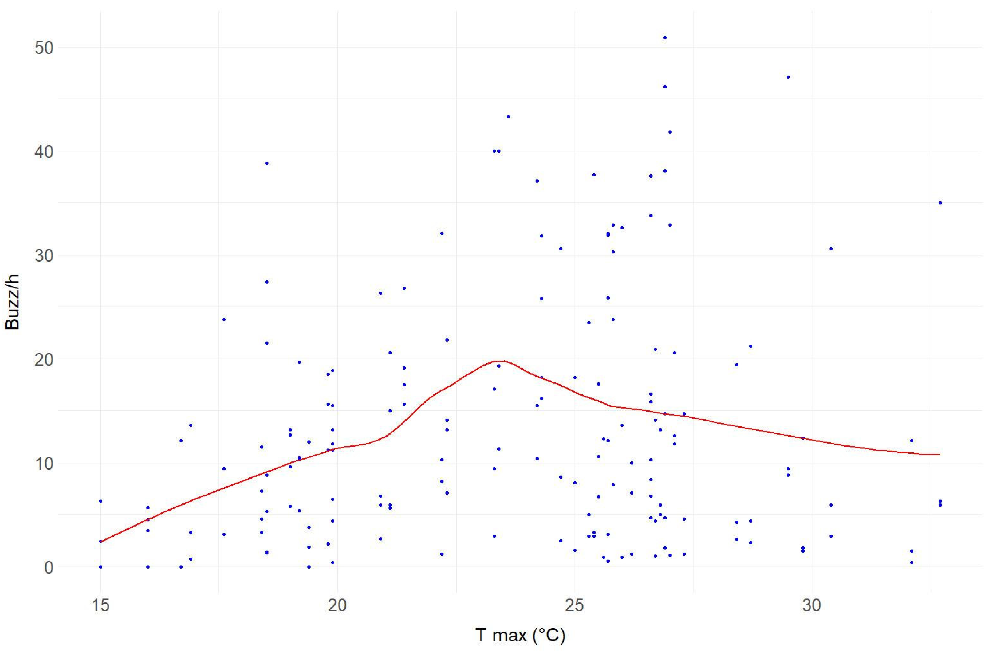
| T Max (°C) | Mean Buzz/h ± SE |
|---|---|
| 15–20 | 8.72 ± 1.11 |
| 20–25 | 17.30 ± 1.86 |
| 25–30 | 16.53 ± 2.06 |
| 30+ | 11.16 ± 4.25 |
Disclaimer/Publisher’s Note: The statements, opinions and data contained in all publications are solely those of the individual author(s) and contributor(s) and not of MDPI and/or the editor(s). MDPI and/or the editor(s) disclaim responsibility for any injury to people or property resulting from any ideas, methods, instructions or products referred to in the content. |
© 2023 by the authors. Licensee MDPI, Basel, Switzerland. This article is an open access article distributed under the terms and conditions of the Creative Commons Attribution (CC BY) license (https://creativecommons.org/licenses/by/4.0/).
Share and Cite
Alberti, S.; Stasolla, G.; Mazzola, S.; Casacci, L.P.; Barbero, F. Bioacoustic IoT Sensors as Next-Generation Tools for Monitoring: Counting Flying Insects through Buzz. Insects 2023, 14, 924. https://doi.org/10.3390/insects14120924
Alberti S, Stasolla G, Mazzola S, Casacci LP, Barbero F. Bioacoustic IoT Sensors as Next-Generation Tools for Monitoring: Counting Flying Insects through Buzz. Insects. 2023; 14(12):924. https://doi.org/10.3390/insects14120924
Chicago/Turabian StyleAlberti, Simona, Gianluca Stasolla, Simone Mazzola, Luca Pietro Casacci, and Francesca Barbero. 2023. "Bioacoustic IoT Sensors as Next-Generation Tools for Monitoring: Counting Flying Insects through Buzz" Insects 14, no. 12: 924. https://doi.org/10.3390/insects14120924