Prediction and Analysis of Tensile Properties of Austenitic Stainless Steel Using Artificial Neural Network

Abstract

Predicting mechanical properties of metals from big data is of great importance to materials engineering. The present work aims at applying artificial neural network (ANN) models to predict the tensile properties including yield strength (YS) and ultimate tensile strength (UTS) on austenitic stainless steel as a function of chemical composition, heat treatment and test temperature. The developed models have good prediction performance for YS and UTS, with R values over 0.93. The models were also tested to verify the reliability and accuracy in the context of metallurgical principles and other data published in the literature. In addition, the mean impact value analysis was conducted to quantitatively examine the relative significance of each input variable for the improvement of prediction performance. The trained models can be used as a guideline for the preparation and development of new austenitic stainless steels with the required tensile properties.

1. Introduction

Metallic materials are widely used in daily life, especially a variety of steel that have a very long history of research. It is known that there are many variables that can affect the properties of steels such as strength [1]. Strength is the ability of a material to resist plastic deformation or fracture, and the strength properties such as tensile strength and plasticity of steels are usually dependent on chemical composition. In addition, the heat treatments, such as annealing, tempering and quenching, can effectively control the microstructure, grain size and defects, which are all closely related to the tensile properties of steels. In addition, the tensile properties are also affected by the service conditions such as working temperature and irradiation environment [2]. To discover the inherent mechanism of how these variables affect the steels, researchers could only get the preliminary influence trends through the continuous experiments via changing a part of variables for a long time. A formula obtained with the traditional linear fitting regression is generally difficult to capture the exact correlations between relative variables and corresponding properties of steels, because they often have complex nonlinear relationships [3].

With the vigorous development of computer technology, machine learning sprang up and became a powerful method for finding the patterns in high-dimensional data [4]. Machine learning is actually an efficient statistical analysis method to capture the linear or nonlinear internal relationships by learning from empirical data [5]. The common machine learning methods include artificial neural network (ANN) [6,7], support vector machine (SVM) [8,9], decision tree (DT) [10] and so on. Nowadays, machine learning prompts data science and analytics to become a significant tool to find the desired causal relations in the material research [11], and results in developing a new field termed as “Materials Informatics” [12,13] in recent years. Machine learning has been rapidly used in the fields of metals [14,15,16,17,18], as well as polymers [19], semiconductors [20,21], which fully demonstrates its powerful universality.

Meanwhile, in order to meet the needs of machine learning for big data [22], many experimental data were collected and established databases such as MatNavi [23], MatWeb [24] and Matmatch [25]. MatNavi contains a large amount of data about the fatigue and creep properties of various steels, which have been already used for machine learning model establishment and research. Agrawal et al. [26] proved the practicality of machine learning for fatigue strength research with the Fatigue Data Sheet. Sourmail et al. [27] correctly captured the important influence trends using the established models with ANN based on the Creep Data Sheet. Besides the fatigue and creep properties, a few machine learning models have been established to obtain the correlations between the tensile properties of steels and the important variables. Guo et al. [28] used the ANN model to well characterize the relationships between the mechanical properties of maraging steels and composition, processing and working conditions. Fragassa et al. [29] chose the metallographic factors as the input features and designed three kinds of machine learning methods to model the mechanical properties of cast iron.

However, for austenitic stainless steel (ASS), more attention is paid on the creep, fatigue and corrosion resistance [30,31,32]. Besides the corrosion resistance, the mechanical properties such as strength of ASS are also important for their application and have drawn much attention in past decades. The tensile properties of ASS have been extensively studied both experimentally and theoretically. Sivaprasad et al. [33] developed an artificial neural network model to correlate alloy composition and test temperature to tensile properties of 15Cr-15Ni-2.2Mo-Ti modified ASS. Desu et al. [34] used test temperature and strain rates as descriptors to predict the tensile properties of ASS 304L and 316L using the ANN model. However, there are no general machine learning models to correlate chemical composition, heat processes and service conditions to tensile properties of ASS, and clarify how each variable affects the tensile properties of ASS.

In this work, we proposed a machine learning method using ANN to predict the tensile properties of ASS with the chemical composition, solution treatment conditions (heat processes) and test temperature (service condition) as descriptors. The models established by partial data in the database have high predictive accuracy for the remaining data and some new data outside the database. We also calculated the impact degrees of each variable with the mean impact value (MIV) method and predicted the influence trends of several important variables on tensile properties. Our results conform to the previous metallurgical theories, and the established models can guide us for further research and development of new ASS with the expected tensile properties.

2. The Database and ANN Model

2.1. Information of the Database

Our study is based on the tensile test data of some classical types of ASS including SUS 304, SUS 316, SUS 321, SUS 347 and NCF 800H, which is referenced to the Creep Data Sheet of Steel (No.4B, 5B, 6B, 14B, 15B, 26B, 27B, 28B, 32A, 42 and 45) from NIMS MatNavi and BSCC High Temperature Data from The British Steelmakers Creep Committee [35], and collected by the Material Algorithm Project (MAP) of University of Cambridge [36].

The original data contains 1916 samples, of which 1107 samples unfortunately lack the necessary information, so the remaining 809 samples are selected for further research. The data has the following characteristics: (1) Every sample has two kinds of tensile properties as output, yield strength (YS) and ultimate tensile strength (UTS); (2) The data contains 20 variables selected as input: chemical composition, solution treatment conditions and test temperature, as shown in

Table 1. The input variables of austenitic stainless steel in this research.

Number	Variables	Number	Variables
1	Chromium (Cr, wt%)	11	Carbon (C, wt%)
2	Nickel (Ni, wt%)	12	Boron (B, wt%)
3	Molybdenum (Mo, wt%)	13	Phosphorus (P, wt%)
4	Manganese (Mn, wt%)	14	Sulfur (S, wt%)
5	Silicon (Si, wt%)	15	Cobalt (Co, wt%)
6	Niobium (Nb, wt%)	16	Aluminum (Al, wt%)
7	Titanium (Ti, wt%)	17	Solution treatment temperature (Ts, K)
8	Vanadium (V, wt%)	18	Solution treatment time (ts, s)
9	Copper (Cu, wt%)	19	Water-quenched or Air-quenched
10	Nitrogen (N, wt%)	20	Test temperature (Tt, K)

. The chemical composition includes some common elements such as carbon (C), nickel (Ni), chromium (Cr), Nitrogen (N) and the microalloying additions such as titanium (Ti), vanadium (V) and niobium (Nb). The parameters of solution treatment conditions on ASS are temperature and time. It should be noted that after the solution treatment, in order to stabilize the austenite structure and prevent the carbide precipitation at room temperature, it is generally required to perform the rapid water quenching of the materials. Here, the samples that are water-quenched in the database are set as the label 1 and the air-cooled ones without water quenching are set as the label 0. These features are related to the physical metallurgy which is important for modeling and property predictions of ASS [37]. There are some other features in the original database, such as the type of melting, grain size and the form of products, but the data of them are incomplete or they have a lower correlation with tensile properties. So they are not considered in this study. Further information about the input variables is given in

Table A1. The 415 samples with water quenching after solution treatment (label: 1).

Variables	Range	Mean	SD
Cr	16.39%–21.06%	18.31%	1.432%
Ni	8.4%–34.45%	16.4%	9.078%
Mo	0%–2.65%	0.95%	1.114%
Mn	0.81%–1.75%	1.39%	0.3088%
Si	0.39%–0.82%	0.585%	0.1194%
Nb	0%–0.79%	0.0749%	0.2004%
Ti	0%–0.53%	0.188%	0.2098%
V	0%–0.057%	0.0071%	0.0166%
Cu	0%–0.35%	0.139%	0.1101%
N	0%–0.081%	0.0197%	0.01422%
C	0.012%–0.1%	0.0607%	0.01556%
B	0%–0.003%	0.0005%	0.00058%
P	0%–0.038%	0.0214%	0.00858%
S	0%–0.05%	0.011%	0.00829%
Co	0%–0.54%	0.115%	0.152%
Al	0%–0.52%	0.124%	0.188%
Ts	1323–1473 K	1378 K	42.79 K
ts	120–7200 s	2414 s	2397.2 s
Tt	293–1273 K	731 K	267.42 K

and

Table A2. 394 samples with air quenching after solution treatment (label: 0).

Variables	Range	Mean	SD
Cr	15.9%–18.3%	17.57%	0.4594%
Ni	9.15%–12.4%	11.1%	1.0906%
Mo	0%–2.72%	0.856%	1.1288%
Mn	0.79%–1.71%	1.386%	0.2784%
Si	0.29%–0.84%	0.482%	0.1335%
Nb	0%–0.9%	0.128%	0.2936%
Ti	0%–0.56%	0.221%	0.2286%
V	0%–0% 2	0%	0%
Cu	0%–0%	0%	0%
N	0%–0%	0%	0%
C	0.02%–0.1%	0.053%	0.01167%
B	0%–0.004%	0.000081%	0.00056%
P	0%–0.04%	0.0209%	0.00711%
S	0%–0.028%	0.0158%	0.00646%
Co	0%–0%	0%	0%
Al	0%–0%	0%	0%
Ts	1293–1403 K	1348 K	32.7514 K
ts	120–3600 s	2117 s	1149.61 s
Tt	293–973 K	626 K	221.568 K

² The 394 samples with air quenching have the chemical composition except V, Cu, N, Co and Al.

of Appendix A.

2.2. Division of Data and Pre-Processing

The data are randomly divided into two groups. Eight-three percent of the data (674 samples) are selected as the training set for the model establishment while the remaining 17% (135 samples) are employed as the testing set for accuracy verification of models, which makes the training/testing ratio close to 5/1.

Deeply understanding and pre-processing the data with appropriate normalization before modeling is one of the most vital steps of effective data mining [26]. The input data generally have more than one dimension and each variable has different size of range, so it is necessary to make each variable normalized within the range from 0 to 1 using the following equation firstly to improve the accuracy and efficiency of calculation and prediction:

$${\mathrm{x}}_{\mathrm{n}}=\left({\mathrm{x}-\mathrm{x}}_{\min }\right)/\left({\mathrm{x}}_{\mathrm{Max}}{-\mathrm{x}}_{\min }\right),$$

(1)

where x_n is the normalized value of the corresponding x, x_Max and x_min are the maximum and minimum values of x respectively.

2.3. ANN Model Development

Artificial neural network (ANN) is a flexible model for non-linear statistical analysis and it can be used for both data classification and regression calculation. It looks like a box that links input data and output data together via a set of non-linear functions. More details of this method can be found elsewhere [38], but it is necessary to have a brief introduction on the main features of ANN.

A simple three-layer feedforward network is competent for general works, such as the one shown in Figure 1. As the name suggests, it consists of three layers: input, hidden and output. The transfer function in the second layer can be any kind of non-linear function as long as it is continuous and differentiable, such as the hyperbolic tangent function tanh (Equation (2)), which can effectively capture the interaction between the inputs and map many functions of practical interest [39]. The transfer function in the third layer is usually linear (Equation (3)):

$${\mathrm{h}}_{\mathrm{i}}=\tan \mathrm{h}\left({\displaystyle \sum }_{\mathrm{j}}{\mathrm{w}}_{\mathrm{ij}}^{\left(1\right)}{\mathrm{x}}_{\mathrm{j}}{+\mathsf{\theta }}_{\mathrm{i}}^{\left(1\right)}\right),$$

(2)

$$\mathrm{y}={\displaystyle \sum }_{\mathrm{i}}{\mathrm{w}}_{\mathrm{ij}}^{\left(2\right)}{\mathrm{h}}_{\mathrm{i}}{+\mathsf{\theta }}^{\left(2\right)},$$

(3)

where x_i are inputs, w_i the weights which determine the strength of the transfer function and the biases h_i the analogous just like the constant in linear regression. The number of neurons in the hidden layer determines the complexity of the model and intensely influences the effect of modeling. How to determine it will be introduced later.

We generally take the following 6 steps for the ANN model development: (1) determine the input and output variables and collect the data; (2) pre-process the data such as normalizing; (3) divide the original database into the training set and testing set; (4) use the training set for modeling; (5) test the established model with the testing set; (6) use the model for further simulation and prediction.

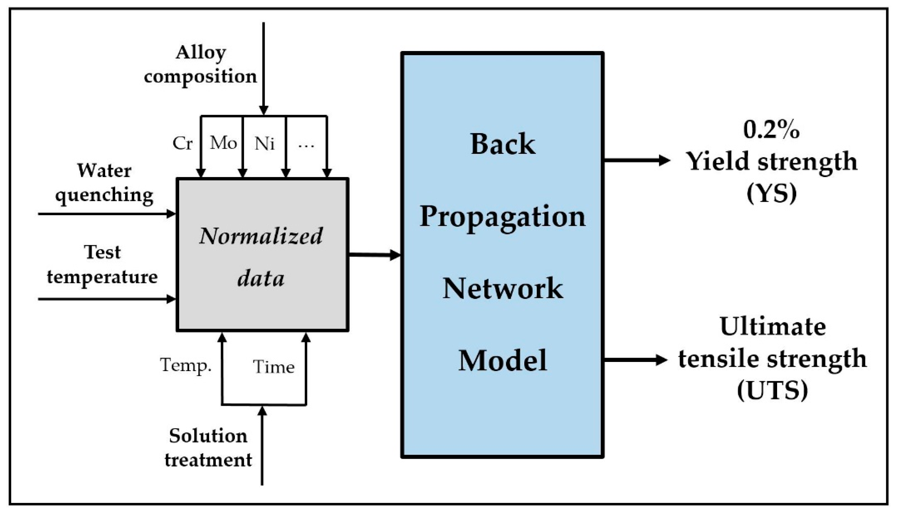
There are many types of network models and what we use in this work is the one based on the back propagation learning algorithm which is called BPNN [40,41]. The traditional algorithms of BPNN usually make the model inaccurate and reduce the efficiency of calculation. Therefore, some kinds of new algorithms start to be widely used with the technological advancement. What we select is one of the most popular algorithms with good generalization called Bayesian regularization (TRAINBR) [42]. The transfer functions we select are the hyperbolic tangent sigmoid function (TANSIG) in the second layer and the linear function (PURELIN) in the third layer. The combination of these functions can meet the basic modeling requirement. To implement the ANN modeling, we use the Neural Network Toolbox (nntool) of MATLAB (R2018b edition) on PC, and TRAINBR, TANSIG, PURELIN are the MATLAB commands of nntool. Some detailed information can be viewed in the manual of MATLAB nntool [43]. In order to describe the modeling process more intuitively, a schematic diagram of the model is illustrated in Figure 2.

As mentioned above, a three-layer network with one hidden layer is found to be sufficient for this study. A suitable neural network usually needs to have a high accuracy and good correction on both the training and testing set. However, it is difficult to select the best architecture of network. Although the model has a very good description of the training set, the accuracy of prediction could be very poor for other new data in the testing set. This phenomenon is generally called overfitting.

Since we have already determined 20 variables as the input and 2 properties as the output, the number of units in the hidden layer will greatly change the architecture and performance of the networks. We determine the optimal number of units in the hidden layer by comparing the predictive accuracy of different networks on the testing set. Here, we use root mean square error (RMSE) and correlation coefficient (R) as the error statistical parameters. The RMSE can accurately measure the deviation between original values and predicted ones, and the R is able to provide information on the strength of correlation between them. They are calculated using the following equation:

$$\mathrm{RMSE}=\sqrt{\frac{1}{\mathrm{n}}{\displaystyle \sum }_{\mathrm{i}=1}^{\mathrm{n}}{\left(\mathrm{f}\left({\mathrm{x}}_{\mathrm{i}}\right){-\mathrm{y}}_{\mathrm{i}}\right)}^2},$$

(4)

$$\mathrm{R}=\frac{{{\displaystyle \sum }}_{\mathrm{i}=1}^{\mathrm{n}}(\mathrm{f}\left({\mathrm{x}}_{\mathrm{i}}\right)-\overline{\mathrm{f}\left(\mathrm{x}\right)})({\mathrm{y}}_{\mathrm{i}}-\overline{\mathrm{y}})}{\sqrt{{{\displaystyle \sum }}_{\mathrm{i}=1}^{\mathrm{n}}{(\mathrm{f}\left({\mathrm{x}}_{\mathrm{i}}\right)-\overline{\mathrm{f}\left(\mathrm{x}\right)})}^2}\sqrt{{{\displaystyle \sum }}_{\mathrm{i}=1}^{\mathrm{n}}{({\mathrm{y}}_{\mathrm{i}}-\overline{\mathrm{y}})}^2}}$$

(5)

where n is total number of data, y_i the original values, ${\mathrm{f}(\mathrm{x}}_{\mathrm{i}})$ the predicted ones, $\overline{\mathrm{f}\left(\mathrm{x}\right)}=\frac{1}{\mathrm{n}}{{\displaystyle \sum }}_{\mathrm{i}=1}^{\mathrm{n}}{\mathrm{f}(\mathrm{x}}_{\mathrm{i}})$ and $\overline{\mathrm{y}}=\frac{1}{\mathrm{n}}{{\displaystyle \sum }}_{\mathrm{i}=1}^{\mathrm{n}}{\mathrm{y}}_{\mathrm{i}}$, respectively [26]. Once the predicted values and the original ones have a small deviation, a strong correlation is found with a small value of RMSE and R close to 1.

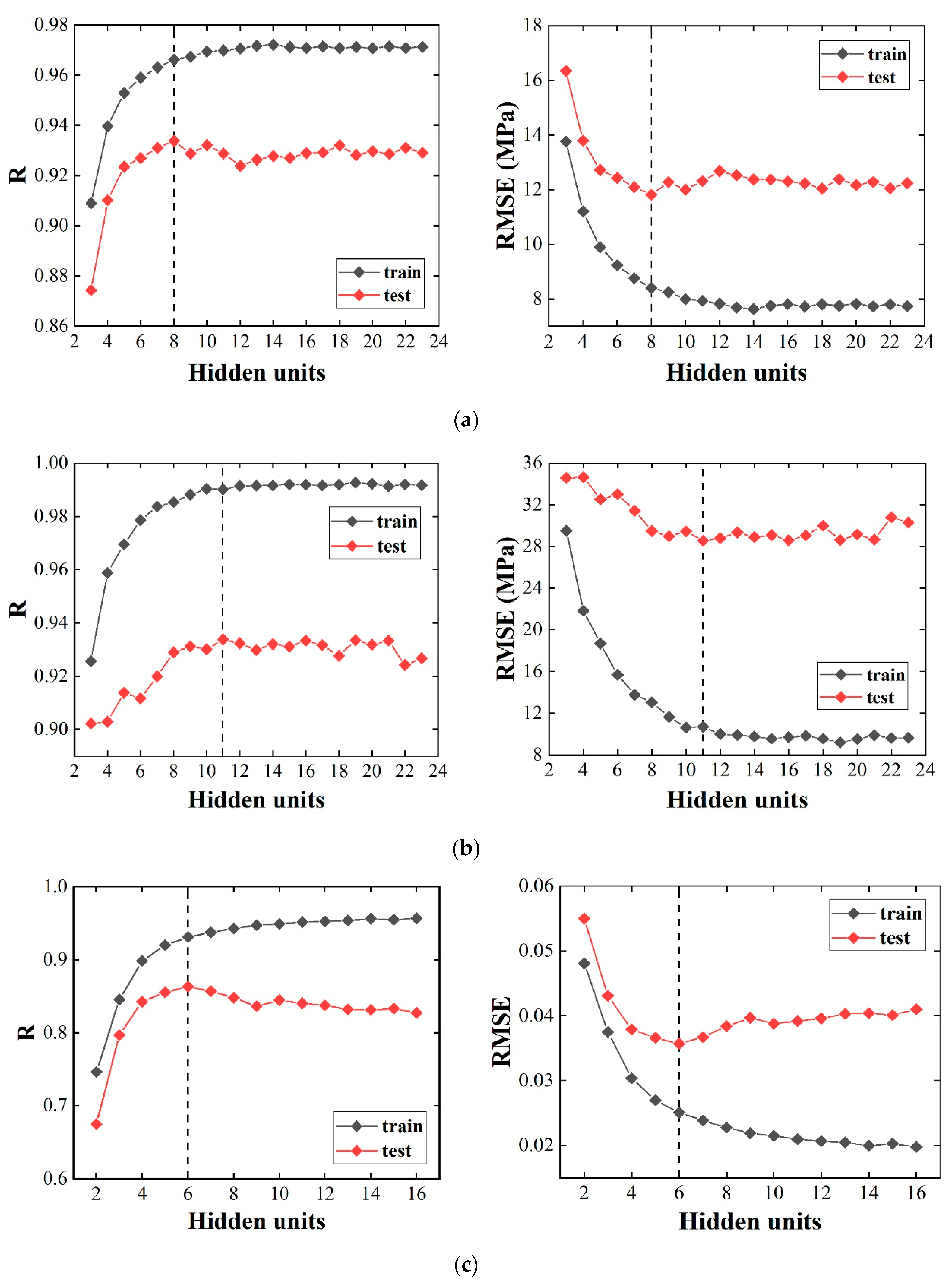
Figure 3a–c shows the values of RMSE and R for YS, UTS and YS/UTS ratio, respectively, with different numbers of the hidden units of the training and testing set. The increase in number of hidden units means the more complexity of the model. It is obviously seen that both for YS and UTS, R increases and RMSE decreases in the training set, indicating that the more complicated model has better prediction for the training set. However, a high degree of complexity probably causes the overfitting and makes the model not suitable for the unseen data in the testing set. As shown in Figure 3, the prediction for the testing set first becomes better and then gets slightly worse when the number of units in the hidden layer increases. Hence, we set the optimum number of units by the RMSE and R of the testing set in this study and it is clearly found to be 8 for YS and 11 for UTS in Figure 3. The architectures of the models we use in the following work are [20-8-1] for YS and [20-11-1] for UTS. The YS/UTS ratio is also an important parameter of tensile properties that determines the reliability of metallic materials [44]. We also establish the network for the YS/UTS ratio and find the similar phenomenon of prediction from the observation of Figure 3c. Its optimum architecture is [20-6-1].

3. Results and Discussion

3.1. Model Performance and Validation

In order to verify the accuracy of the established models, besides the RMSE and R, another goodness-of-fit statistical parameter is the mean absolute percentage error (MAPE) [26], which is used to measure the error between the predicted and original values, and it particularly considers the ratio of error to the original values. The smaller the MAPE value, the higher the predictive accuracy. The value of MAPE is calculated as following equation:

$$\mathrm{MAPE}=\frac{1}{\mathrm{n}}{\displaystyle \sum }_{\mathrm{i}=1}^{\mathrm{n}}\left|\frac{\mathrm{f}\left({\mathrm{x}}_{\mathrm{i}}\right){-\mathrm{y}}_{\mathrm{i}}}{{\mathrm{y}}_{\mathrm{i}}}\right|.$$

(6)

Table 2. Statistical parameters for the training and testing set with the optimal hidden units.

Tensile Properties	Hidden Units	Training			Testing
		(83% of the Data)			(17% of the Data)
		MAPE	RMSE	R	MAPE	RMSE	R
		(%)	(MPa)		(%)	(MPa)
YS	8	4.09	8.40	0.97	5.21	11.82	0.93
UTS	11	1.76	10.69	0.99	3.56	28.54	0.93
YS / UTS	6	4.80	0.025 1	0.93	5.91	0.035 1	0.86

¹ There is no unit for the predicted RMSE of YS/UTS ratio.

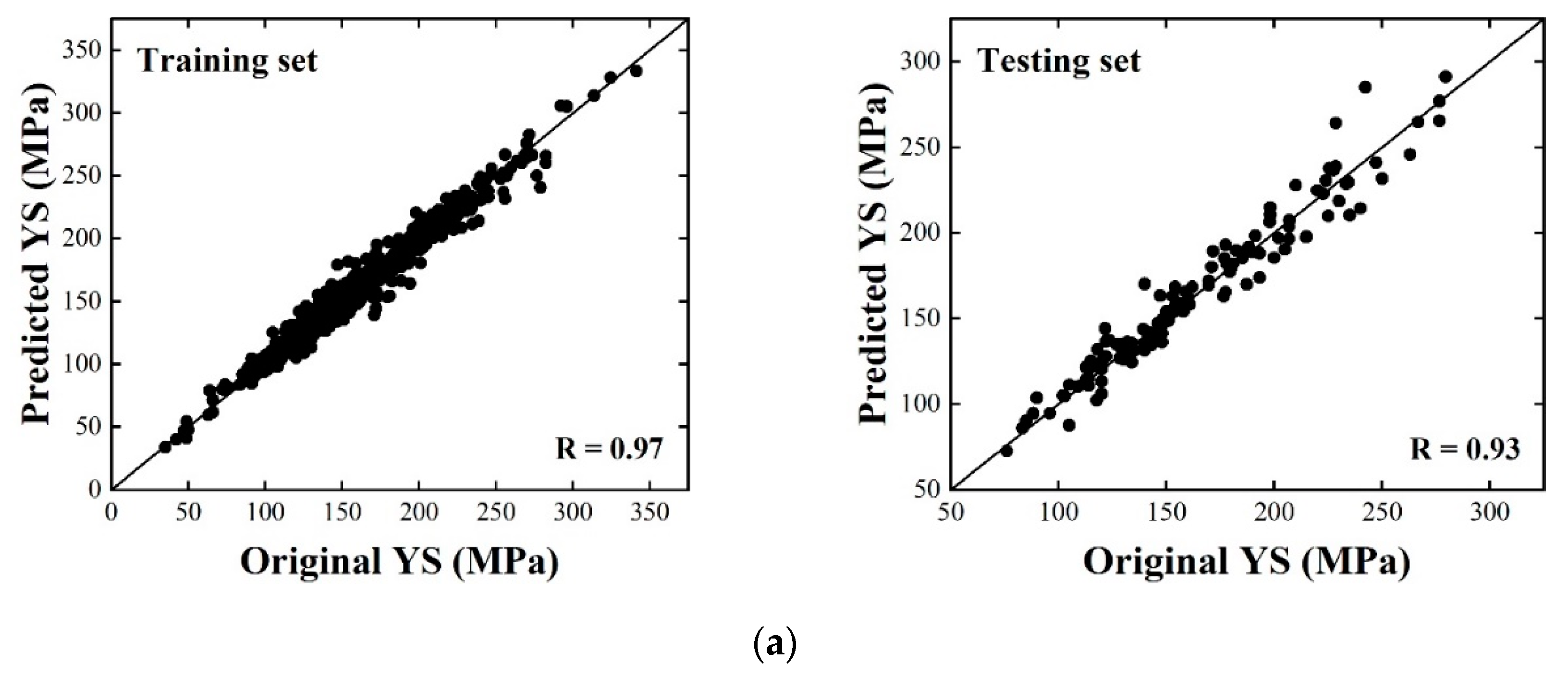
shows the values of MAPE, RMSE and R of ANN models for three tensile properties, YS, UTS and YS/UTS, of the training and testing sets with the optimal hidden units. As it can be seen that the predictions of the training set are generally better than those of the testing set, which could be expected because the model is better for predicting the known data than the unseen data. However, for the testing set, the values of MAPE are less than 6% and of R are above 0.86 for the properties YS, UTS and YS/UTS, indicating a good prediction performance of the models. It is worth noting that the value of R for UTS is nearly 0.99, indicating that the present model has a more accurate description and prediction for UTS than YS and YS/UTS. Figure 4 shows the original and predicted values of UTS, YS and YS/UTS for the training and testing sets. Good performance of the models for UTS, YS and YS/UTS is observed for both the training and testing sets.

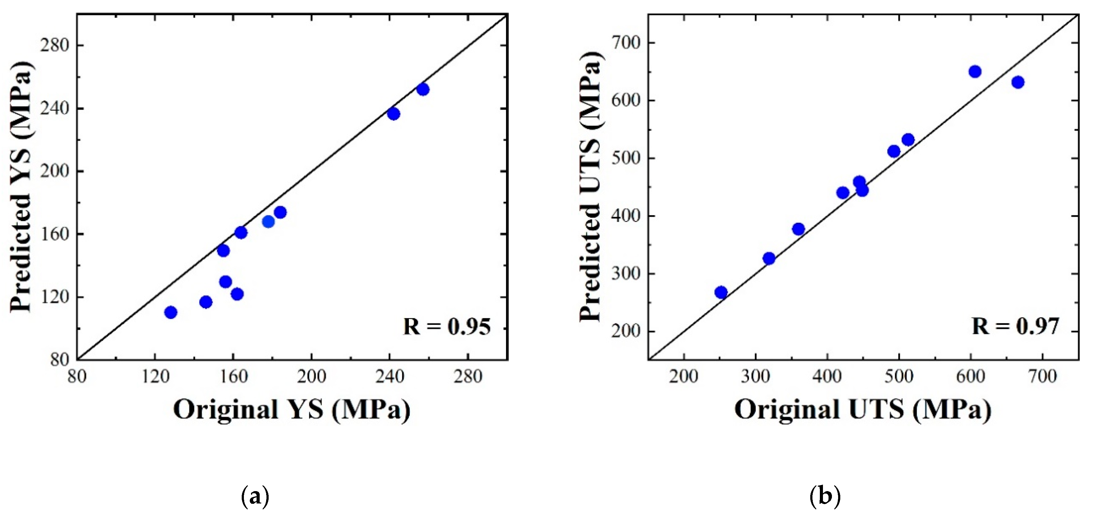
In order to verify the ability of established models to predict the unseen data outside the database, some new data of tensile properties of ASS in the Fatigue Data Sheet from MatNavi are tested. The details of these data are listed in

Table A3. The variables of new unseen data of austenitic stainless steel.

Variables	No.15 (SUS 316)	No.42 (SUS 304)
Cr	17.05%	18.53%
Ni	12.6%	9.1%
Mo	2.24%	0.12%
Mn	1.1%	0.88%
Si	0.7%	0.54%
Nb	0.001%	0%
Ti	0.03%	0.02%
V	0%	0%
Cu	0.31%	0.06%
N	0.017%	0.023%
C	0.05%	0.05%
B	0.003%	0%
P	0.033%	0.029%
S	0.003%	0.01%
Co	0%	0.21%
Al	0.02%	0.023%
Ts	1373 K	1373 K
ts	1800 s	1800 s
Water or air quenching	Water quenching (label: 1)	Water quenching (label: 1)
Tt	298, 673, 773, 873, 973 K	298, 673, 773, 873, 973 K

of Appendix A. The prediction results are shown in Figure 5 and the statistical parameters are presented in

Table 3. Statistical parameters of predicted results for the new data.

Tensile Properties	MAPE (%)	RMSE (MPa)	R
YS	9.61	5.27	0.95
UTS	4.16	6.06	0.97

. It can be seen from Figure 5 and Table 3 that the models have good performance for UTS and YS with R ≥ 0.95. This means that the models have a good ability to predict the unknown data. Moreover, the models have a relative better prediction for UTS than YS with these new data, which is similar to the result for the original data mentioned above.

3.2. Feature Analysis

3.2.1. Mean Impact Value

Using machine learning cannot only make accurate predictions, but also further analyze the effect of each single variable on the corresponding properties. The mean impact value (MIV) method has been widely used for quantitative feature analysis in the machine learning application to explore the relative importance of each input variable for the improvement of the prediction performance [45]. The algorithm process of MIV is as follow:

• Building two new datasets by varying the magnitude of one of variables by $\pm$10% for the original training set;
• Inputting two new datasets as the simulation samples to the model and obtaining two predicted results;
• Calculating the difference value of these two predicted results, called the impact value (IV);
• According to the amount of samples in the original training set, calculating the average value of IV, that is MIV of each variable;
• Repeating the above steps in turn to get the MIV of each independent variable. It should be noted that the value of MIV indicates the positive or negative effect as well as the intensity of influence.

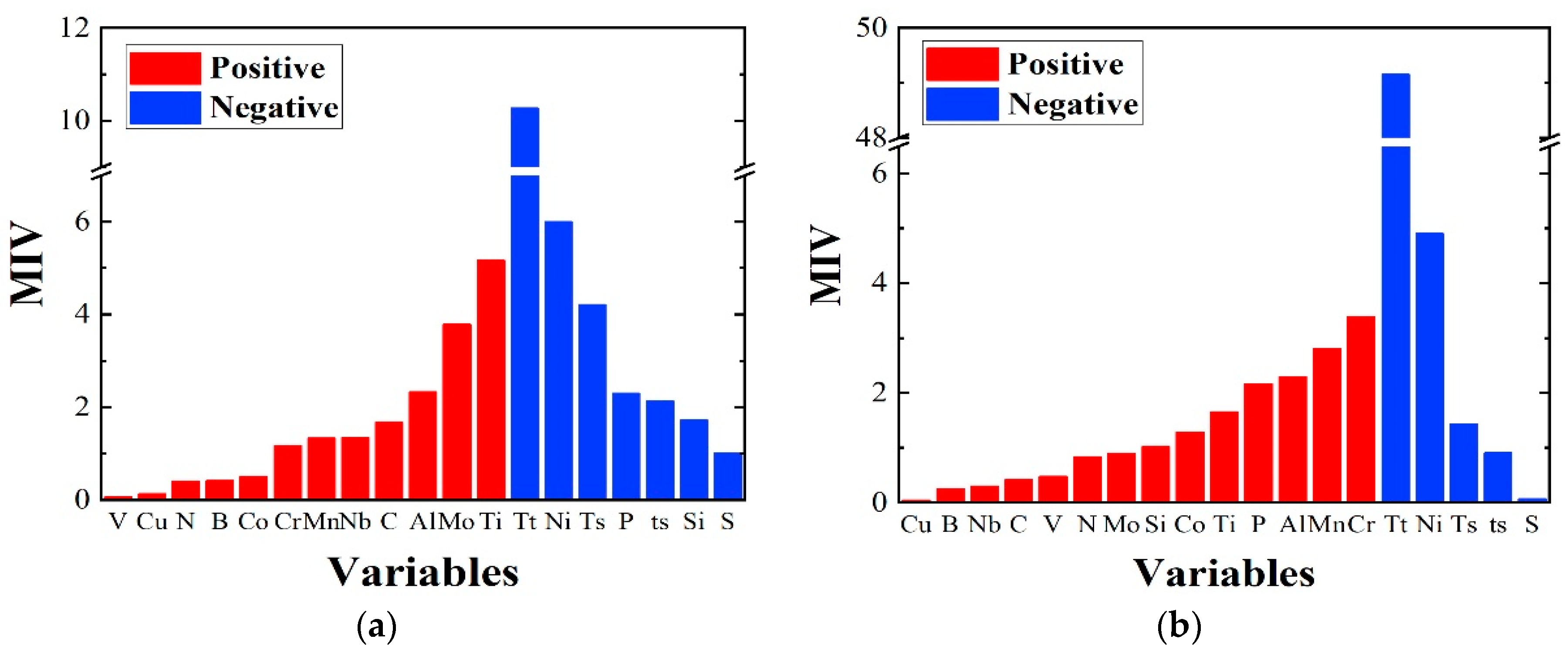
The MIV values of each variable are calculated and shown in Figure 6. MIV results show that test temperature and Ni content are two most important factors for both YS and UTS. Generally, the tensile properties of steels largely depend on the test temperatures and experimentally, the properties often need to be carried out at different test temperatures. Moreover, for the UTS, besides the test temperature, the importance of Ni and Cr contents is in good agreement with the traditional metallurgical theories and the engineering practice. In ASS steels, Ni and Cr are intentionally added in large quantities into ASS to improve the tensile properties and high-temperature oxidation resistance. In addition, Ti and Mo contents and temperature of solution treatment are also strong indicators of YS, while Cr and Mn contents are highly related to UTS. Note that the MIV value of test temperature for UTS is much greater than that for YS, which means that the test temperature has a much stronger effect on UTS than YS.

The information about the positive and negative correlation between the properties and all features is also shown in Figure 6. The elements Cr, V, Ti, Mo, Nb, C and Mn appear positively correlated with YS and UTS, which is consistent with the characteristics of previous theories of precipitation strengthening and solid solution strengthening [2,46]. The elements Cr, V, Ti, Mo and Nb could form strong carbides or nitrides that play a role of second phase precipitation strengthening. The elements like C, N and Mn could form interstitial solid solution that lead to the solid solution strengthening. In addition, it is worth mentioning that S content, test temperature and solution treatment time all exhibit the negative influences on YS and UTS.

3.2.2. Influence Trends of Variables

As discussed above, the present models show good prediction performance for the tensile properties YS and UTS, so they can be used to predict the influence trends of some important variables on the properties. Here, the effects of some typical elements and treatment conditions are examined. To investigate the effect of each variable, a new dataset is built and the values of this variable are set from the maximum to minimum and the values of other variables are set to the average of the original database, which are listed in Table A1 of Appendix A.

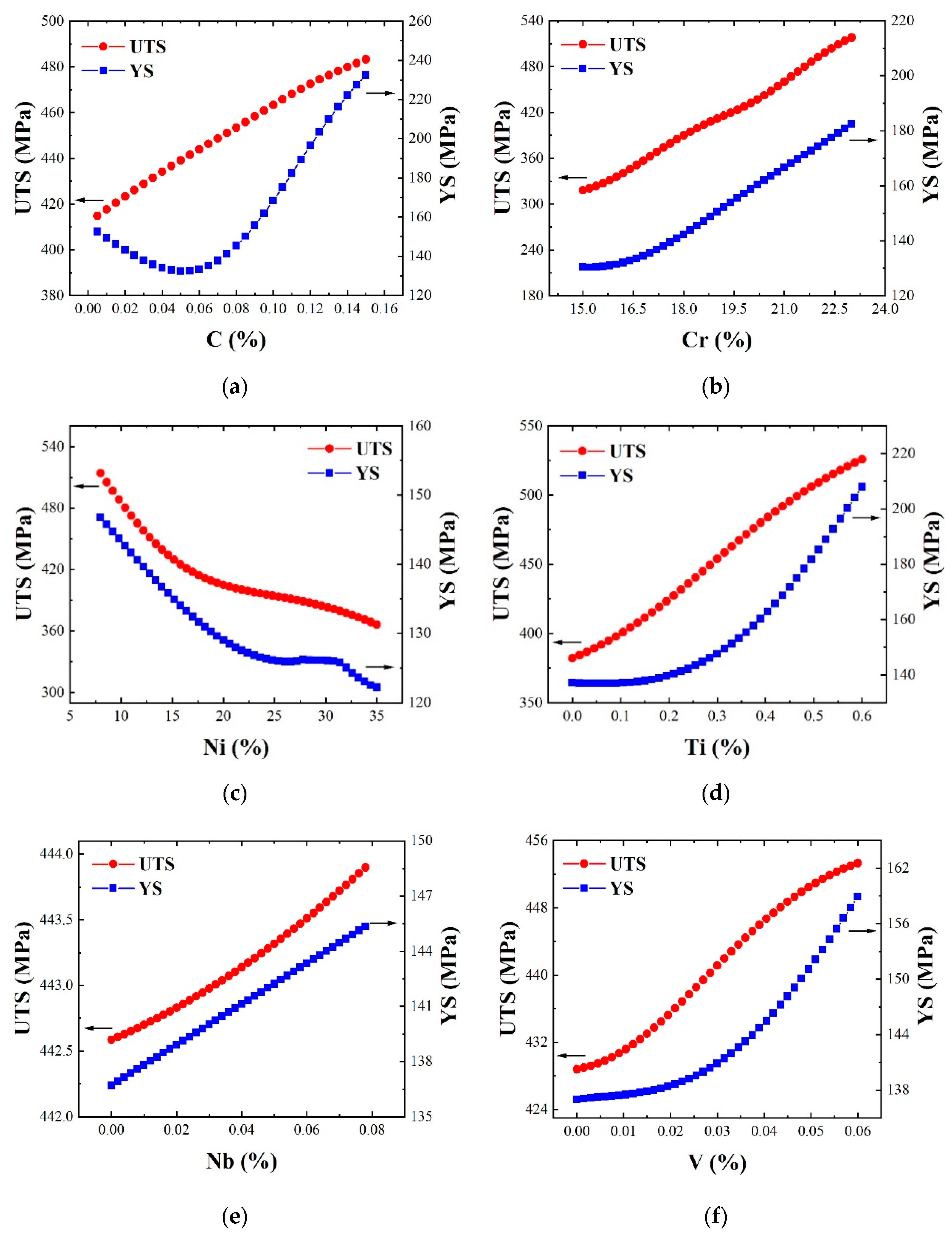
Figure 7 shows the effect of typical elements C, Cr, Ni, Ti, Nb, and V on the tensile properties UTS and YS. It can be observed that both UTS and YS generally show positive correlations with the contents of C, Cr, Ti, Nb and V, while they exhibit negative correlation with the Ni content. The results are in good agreement with the above MIV analyses that C and Cr are added to stabilize the austenite and to form interstitial solid solution or carbides dispersed in the matrix [2,46,47]. Note that for YS, it shows a firstly decreasing trend when the C content is less than 0.05%. This result is probably due to the lack of sufficient amount of data that limits the accuracy of the model. Moreover, the reduced value is not large and the overall tendency is still increasing, so the model has a reasonable prediction result for the effect of C content on YS within a certain error tolerance. The microalloying elements Ti, Nb and V could form the stable second carbides to prevent austenite grain coarsening, hindering the dislocation motion and then strongly strengthening the mechanical properties of ASS. Previous experimental results show that Nb and Ti can improve the tensile properties of ASS [48]. As shown in Figure 7c, Ni is a deliberate element which has a strong negative correlation with tensile strengths and makes ASS have good plasticity and ductility for subsequent processing [49].

It is known that by solution treatment, the second phase carbon nitride could be uniformly dispersed in the matrix and then leads to increased second phase strengthening. However, the continued solution treatment will cause the grain coarsening and the reduction of crystal defects of ASS. So, the effect of second phase strengthening is gradually offset and the strength of ASS decreases ultimately [50,51,52]. Figure 8 presents the effect of T_s, t_s and T_t on the tensile properties UTS and YS. The results show when the solution treatment conditions are located at [1323~1473 K, 2414 s] or [1378 K, 120–7200 s], both UTS and YS generally show a decreasing trend with increasing T_s and t_s. Under this situation, the effects of grain coarsening and reduction of defects offset the second phase strengthening. In Figure 8c, both UTS and YS decrease as T_t increases. When the temperature is close to 1300 K, the predicted value of UTS reduces to nearly 0 and even less than YS. This is clearly contrary to previous theories, which is similar to the previous prediction for the influence trend of carbon. The possible reason is a lack of sufficient data. By comparing the predicted results in Figure 7 and Figure 8, the test temperature is the most influential variable for YS and UTS, where the variations of tensile properties are the largest, especially for UTS. This is also consistent with the conclusion of the MIV analysis above.

4. Conclusions

In this work, we have developed two BPNN models capable of studying and predicting two tensile properties of austenitic stainless steel, YS and UTS, as a function of 20 variables including chemical composition, heat treatment conditions and test temperature. The accuracy of the established models is evaluated based on three statistical parameters, RMSE, R and MAPE. The results indicate that the models have not only highly predictive accuracy on both the training and testing set, but also have good prediction performance for some unknown data. For analyzing the effect of each variable on YS and UTS, we use the MIV method and predict the influence trends of several important variables with the established models. The results correctly reflect the positive and negative correlation between the tensile properties and all features, which are consistent with the previous metallurgical theories.

Compared with experiments and other models, the present models are able to accurately predict the tensile properties of ASS when all features are known. Based on the models, the test temperature and Ni content are found to be two most important factors for both YS and UTS. This work is helpful for the preparation and development of new ASS in the future.

References

1. Callister, W.D.; Rethwisch, D.G. Materials Science and Engineering: An Introduction; John Wiley & Sons: New York, NY, USA, 2007; Volume 7. [Google Scholar]
2. Krauss, G. Steels: Processing, Structure, and Performance; ASM International: Russell, OH, USA, 2015. [Google Scholar]
3. Reifsnider, K.L.; Tamuzs, V. On nonlinear behavior in brittle heterogeneous materials. Compos. Sci. Technol. 2006, 66, 2473–2478. [Google Scholar] [CrossRef]
4. Liu, Y.; Zhao, T. Materials discovery and design using machine learning. J. Mater. 2017, 3, 159–177. [Google Scholar] [CrossRef]
5. Murphy, K.P. Machine Learning: A Probabilistic Perspective; MIT Press: Cambridge, MA, USA, 2012. [Google Scholar]
6. Bishop, C.M. Neural Networks for Pattern Recognition; Oxford University Press: Oxford, UK, 1995. [Google Scholar]
7. Zurada, J.M. Introduction to Artificial Neural Systems; West Publishing Company: St. Paul, MN, USA, 1992; Volume 8. [Google Scholar]
8. Cortes, C.; Vapnik, V. Support-vector networks. Mach. Learn. 1995, 20, 273–297. [Google Scholar] [CrossRef]
9. Vapnik, V. The Nature of Statistical Learning Theory; Springer Science & Business Media: New York, NY, USA, 2013. [Google Scholar]
10. Rokach, L.; Maimon, O.Z. Data Mining with Decision Trees: Theory and Applications; World Scientific: Singapore, 2008; Volume 69. [Google Scholar]
11. Council, N.R. Integrated Computational Materials Engineering: A Transformational Discipline for Improved Competitiveness and National Security; National Academies Press: Washington, DC, USA, 2008. [Google Scholar]
12. Kalidindi, S.R.; Niezgoda, S.R. Microstructure informatics using higher-order statistics and efficient data-mining protocols. Jom 2011, 63, 34–41. [Google Scholar] [CrossRef]
13. Rajan, K. Materials informatics. Mater. Today 2005, 8, 38–45. [Google Scholar] [CrossRef]
14. Ward, L.; O’Keeffe, S.C. A machine learning approach for engineering bulk metallic glass alloys. Acta Mater. 2018, 159, 102–111. [Google Scholar] [CrossRef]
15. Xue, D.; Balachandran, P.V. Accelerated search for materials with targeted properties by adaptive design. Nat. Commun. 2016, 7, 11241. [Google Scholar] [CrossRef] [Green Version]
16. Lin, Y.; Zhang, J. Application of neural networks to predict the elevated temperature flow behavior of a low alloy steel. Comput. Mater. Sci. 2008, 43, 752–758. [Google Scholar] [CrossRef]
17. Murugesan, M.; Sajjad, M. Hybrid Machine Learning Optimization Approach to Predict Hot Deformation Behavior of Medium Carbon Steel Material. Metals 2019, 9, 1315. [Google Scholar] [CrossRef] [Green Version]
18. Kurt, H.; Oduncuoglu, M. A mathematical formulation to estimate the effect of grain refiners on the ultimate tensile strength of Al-Zn-Mg-Cu alloys. Metals 2015, 5, 836–849. [Google Scholar] [CrossRef] [Green Version]
19. Mannodi-Kanakkithodi, A.; Pilania, G. Machine learning strategy for accelerated design of polymer dielectrics. Sci. Rep. 2016, 6, 20952. [Google Scholar] [CrossRef] [PubMed] [Green Version]
20. Irani, K.B.; Cheng, J. Applying machine learning to semiconductor manufacturing. IEEE Expert 1993, 8, 41–47. [Google Scholar] [CrossRef]
21. Yu, L.; Zunger, A. Identification of potential photovoltaic absorbers based on first-principles spectroscopic screening of materials. Phys. Rev. Lett. 2012, 108, 068701. [Google Scholar] [CrossRef] [PubMed]
22. Mayer-Schönberger, V.; Cukier, K. Big Data: A Revolution that Will Transform How We Live, Work, and Think; Houghton Mifflin Harcourt: Boston, MA, USA, 2013. [Google Scholar]
23. NIMS MatNavi. Available online: https://mits.nims.go.jp/index_en.html (accessed on 10 December 2019).
24. MatWeb Material Property Data. Available online: http://www.matweb.com/ (accessed on 15 July 2019).
25. Matmatch. Available online: https://matmatch.com/ (accessed on 22 July 2019).
26. Agrawal, A.; Deshpande, P.D. Exploration of data science techniques to predict fatigue strength of steel from composition and processing parameters. Integr. Mater. Manuf. Innov. 2014, 3, 90–108. [Google Scholar] [CrossRef] [Green Version]
27. Sourmail, T.; Bhadeshia, H. Neural network model of creep strength of austenitic stainless steels. Mater. Sci. Technol. 2002, 18, 655–663. [Google Scholar] [CrossRef]
28. Guo, Z.; Sha, W. Modelling the correlation between processing parameters and properties of maraging steels using artificial neural network. Comput. Mater. Sci. 2004, 29, 12–28. [Google Scholar] [CrossRef] [Green Version]
29. Fragassa, C.; Babic, M. Predicting the tensile behaviour of cast alloys by a pattern recognition analysis on experimental data. Metals 2019, 9, 557. [Google Scholar] [CrossRef] [Green Version]
30. Hodgson, P.D.; Kong, L.X. The prediction of the hot strength in steels with an integrated phenomenological and artificial neural network model. J. Mater. Process. Technol. 1999, 87, 131–138. [Google Scholar] [CrossRef]
31. Ramana, K.; Anita, T. Effect of different environmental parameters on pitting behavior of AISI type 316L stainless steel: Experimental studies and neural network modeling. Mater. Design 2009, 30, 3770–3775. [Google Scholar] [CrossRef]
32. Mandal, S.; Sivaprasad, P. Artificial neural network modeling of composition–process–property correlations in austenitic stainless steels. Mater. Sci. Eng. A 2008, 485, 571–580. [Google Scholar] [CrossRef]
33. Sivaprasad, P.; Mandal, S. Artificial neural network modelling of the tensile properties of indigenously developed 15Cr-15Ni-2.2Mo-Ti modified austenitic stainless steel. Trans. Indian Inst. Met. 2006, 59, 437–445. [Google Scholar]
34. Desu, R.K.; Krishnamurthy, H.N. Mechanical properties of Austenitic Stainless Steel 304L and 316L at elevated temperatures. J. Mater. Res. Technol. 2016, 5, 13–20. [Google Scholar] [CrossRef] [Green Version]
35. The British Steelmakers Creep Committee: BSCC High Temperature Data; The Iron and Steel Institute: London, UK, 1973.
36. Materials Algorithms Project. Available online: https://www.phase-trans.msm.cam.ac.uk/map (accessed on 17 June 2019).
37. Shen, C.; Wang, C. Physical metallurgy-guided machine learning and artificial intelligent design of ultrahigh-strength stainless steel. Acta Mater. 2019, 179, 201–214. [Google Scholar] [CrossRef]
38. Bhadeshia, H. Neural networks in materials science. ISIJ Int. 1999, 39, 966–979. [Google Scholar] [CrossRef]
39. Hornik, K.; Stinchcombe, M. Multilayer feedforward networks are universal approximators. Neural Netw. 1989, 2, 359–366. [Google Scholar] [CrossRef]
40. Hecht-Nielsen, R. Theory of the backpropagation neural network. In Neural Networks for Perception; Academic Press: New York, USA, 1992; pp. 65–93. [Google Scholar]
41. Rumelhart, D.E.; Hinton, G.E. Learning representations by back-propagating errors. Cognitive Modeling. Nature 1986, 323, 533–536. [Google Scholar] [CrossRef]
42. Burden, F.; Winkler, D. Bayesian regularization of neural networks. In Artificial Neural Networks; Humana Press: Totowa, NJ, USA, 2008; pp. 23–42. [Google Scholar]
43. Statistics and Machine Learning Toolbox. Available online: https://www.mathworks.com/products/statistics.html (accessed on 23 December 2019).
44. Bhadeshia, H. Bainite in Steels. Cambridge: The Institute of Materials; The University Press: London, UK, 1992. [Google Scholar]
45. Dombi, G.W.; Nandi, P. Prediction of rib fracture injury outcome by an artificial neural network. J. Trauma Acute Care 1995, 39, 915–921. [Google Scholar] [CrossRef]
46. McGuire, M.F. Stainless Steels for Design Engineers; ASM International: Russell, OH, USA, 2008. [Google Scholar]
47. Martins, L.F.M.; Plaut, R.L. Effect of Carbon on the Cold-worked State and Annealing Behavior of Two 18wt% Cr–8wt% Ni Austenitic Stainless Steels. ISIJ Int. 1998, 38, 572–579. [Google Scholar] [CrossRef]
48. Farahat, A.I.Z.; El-Bitar, T. Effect of Nb, Ti and cold deformation on microstructure and mechanical properties of austenitic stainless steels. Mater. Sci. Eng. A 2010, 527, 3662–3669. [Google Scholar] [CrossRef]
49. Marshall, P. Austenitic Stainless Steels: Microstructure and Mechanical Properties; Springer Science & Business Media: New York, NY, USA, 1984. [Google Scholar]
50. Totten, G.E. Steel Heat Treatment: Metallurgy and Technologies; CRC Press: Boca Raton, FL, USA, 2006. [Google Scholar]
51. Yin, R. Metallurgical Process Engineering; Springer Science & Business Media: New York, NY, USA, 2011. [Google Scholar]
52. Wu, H.; Yang, B. Effect of Solution Temperature on the Microstructure and Mechanical Properties of Wrought 316LN Stainless Steel. Adv. Mater. Res. 2014, 915, 576–582. [Google Scholar] [CrossRef]
Figure 1. Structure of a three-layer feedforward neural network.
Metals 10 00234 g001
Figure 2. Schematic diagram of Back Propagation Neural Network (BPNN) model for predicting two tensile properties of austenitic stainless steels in this study.
Metals 10 00234 g002
Figure 3. The number of units in the hidden layers influences the prediction of models on the training set and testing set: (a) yield strength (YS), (b) ultimate tensile strength (UTS) and (c) YS/UTS ratio. The black and red dots represent correlation coefficient (R) and root mean square error (RMSE) on the training set and testing set, respectively. We use the dotted lines to mark the selection of the optimal number of hidden units in every figure.
Metals 10 00234 g003
Figure 4. Comparison between the predicted and original values on the training set and testing set for: (a) YS, (b) UTS and (c) YS/UTS ratio. X-axis is the original value of tensile properties, Y-axis is the predicted one and the equation of black line in these figures is y = x (The more points concentrated near the black line, the more accurate the predicted values).
Metals 10 00234 g004aMetals 10 00234 g004b
Figure 5. Comparison between the predicted and original values of the unseen data outside the database for: (a) YS and (b) UTS.
Metals 10 00234 g005
Figure 6. The absolute values of mean impact value (MIV) of each variable on two tensile properties: (a) YS and (b) UTS. The red and blue columns represent the positive and negative correlation, respectively (The higher the MIV value, the greater the effect on the corresponding tensile properties).
Metals 10 00234 g006
Figure 7. The predicted influence trends of (a) carbon, (b) chromium, (c) nickel, (d) titanium, (e) niobium and (f) vanadium on YS and UTS. The red and blue dots represent the predicted values of UTS and YS respectively.
Metals 10 00234 g007
Figure 8. The predicted influence trends of (a) temperature, (b) time of solution treatment and (c) test temperature on YS and UTS. The blue and red dots represent the predicted values of YS and UTS respectively.
Metals 10 00234 g008