Abstract
From the point of view of designing materials, it is important to study the complex correlational research that involves measuring several variables and assessing the relation among them. Hence, the notion of machine-oriented data modeling is explored. Among various machine-learning tools, artificial neural networks (ANN) have been used as a stimulating tool to solve engineering-related issues. In this study, the ANN model is designed and trained to correlate the complex relations among composition, temperature and mechanical properties of 25Cr-20Ni-0.4C austenitic stainless steel. The developed model was exploited to estimate the composition–property and temperature–property correlations. The ANN predictions are well suitable for experimental results. The model was able to correlate the complex nature among input and output variables. The model was used to investigate the effect of service temperature on the mechanical properties of 25Cr-20Ni-0.4C steels over a wide temperature range. The effective response of the alloying elements on the mechanical properties of ambient as well as elevated temperatures was quantitatively estimated with the help of the index of relative importance (IRI) method. Hence, this handy technique is the best tool to overcome the designing complications and to develop the components having remarkable properties.
1. Introduction
Austenitic stainless steels are an extraordinary family of alloys that exhibit unique multifunctional properties such as high corrosion resistance combined with impressive mechanical properties, especially ductility [1,2]. The alloys are commercially used for various temperature regimes, from cryogenic to elevated temperatures [2]. Especially, these alloys are prominent candidates for high-temperature parts of power breeding industries, superheater tubes and fired boilers [3,4,5]. These steels are highly recommended for various structural applications for an extended period of time with less maintenance due to their superior mechanical behavior and resistance to aggressive environments [6,7]. However, when the alloys are exposed to gas environments of low or high hydrogen pressures, significant degradation of mechanical properties has been observed. Hence, the mechanical properties and corrosion behavior are the two main salient features of these alloys. Knowing the explicit knowledge about the mechanical response as a function of composition as well as exposure temperature is a question of importance during designing. Hence, it is a challenging task to design the alloys with the desired properties with less cost of experimentation. Increase in experimental trails promote the various cost factors that can affect the manufacturing cost of alloy designing. The existence of non-linearity and uncertainty among the variables limit the use of statistical methods and mathematical equations.
In this regard, the use of computational tools has been increased to understand the complex input–output variable relationships to solve materials science applications [8]. Especially in the case of austenitic stainless steels, various computational tools have been used for modeling of creep strength as well as rupture life [9], creep life [10] and thermomechanical process optimization [11]. Regarding the creep strength and rupture life reported in [9], the authors used various grades of austenitic stainless steels and the neural network model was able to perceive the interactions between the different input variables (composition, test temperature, rupture life and solution treatment temperature). Y. cui et al. [10] proposed the Riedel models for modeling the long term creep damage of various batches of austenitic stainless steels (316LN) as a function of stress, temperature and time. The developed model was able to predict the creep lifetime of steels for longer times with sufficient accuracy. Further, the relationship between the thermomechanical processing parameters (strain level, annealing temperature and time) with the fraction of the low-∑ coincident site lattice (CSL) boundaries of 304 austenitic stainless steels has been modeled using backpropagation neural networks [11]. By optimizing the thermomechanical process parameters, the authors can attain the maximum fraction of low-∑ CSL boundaries, which help to enhance the intergranular properties of materials [11]. However, to the best of the author’s knowledge, there are no relevant reports regarding the modeling of mechanical properties as a function of composition and exposure temperature of 25Cr-20Ni-0.4C austenitic stainless steels. Is has been well reported that the method using neural networks holds significant importance due to its high accuracy in correlating the complex-related input and output variables, as compared with the other regression as well as the mathematical models [12,13]. In principle, the neural networks can learn from training data and generalize overall trends in functional relationships between inputs and output parameters. Although several network architectures and training algorithms are available, the feed-forward neural network with the back-propagation learning algorithm is more commonly used [14]. Therefore, in the present work, we focused on the development of a feed-forward ANN model to predict the properties for a given composition and exposure temperature, and the relationship of the properties with respect to the input variables. Furthermore, the developed model has been used to examine the significance of alloying elements on the mechanical properties of steels.
2. Materials and Methods
The database used in the present study was collected from the National Institute of Materials Science (NIMS) database, Japan (https://mits.nims.go.jp/index_en.html). High-frequency induction furnace was used for melting the components, and the tube-shaped ingots were prepared by centrifugal casting. The chemical composition analysis was carried out for each ingot, and it is tabulated in Table S1 given in the supplementary data. Based on chemical composition, each steel name is designated as TAA to TAS, as shown in Table S1 in the supplementary data. The tensile test specimens (76 mm length and 6mm diameter with 30 mm gauge length) were taken longitudinally from the middle of the wall thickness of centrifugally-cast tubes. The test was carried out at the room and elevated temperatures (up to 1000 °C in steps of 100 °C). The strength and the ductile properties (yield strength (YS), tensile strength (UTS), % elongation (% El) and % reduction area (% RA)) of the steels are reported in Tables S2 and S3, respectively (given in supplementary data). The entire datasets (168) were randomly divided into training (140) and testing (28) datasets. The testing data are represented with bold-face letters with the * symbol and are presented in the supplementary data.
3. Model Establishment: Defining and Developing the ANN Model
ANN is composed of simple components operating in parallel, and the network components are inspired by the regulation of connected neurons in the human brain. Neural networks are typically organized in layers (input, hidden and output layers). The basic principle of neural networks is “trained or attuned so that the specific input leads to a particular target as output”. The detailed description of the ANN modeling in materials science-based research has been reported in several studies [12,14].
Once the input and output variables were selected, the optimum architecture of ANN was obtained with the help of training. The model training mainly involves fitting the network with experimental values so that the computed outputs are coming up with the experimental results. The well-known standard learning algorithm, the backpropagation (BP) method, and the sigmoid transfer function were used to train the model [15,16]. Model training mainly concentrated on minimizing mean square error (MSE), the average training error in output predictions (Etr) given as
where Etr(y) = average error in prediction of training and testing data set for output parameter y. N = Number of datasets, Ti(y) = Targeted output and Oi(y) = Output calculated.
The computer-programming languages, both C and Java, were used in the training program and graphical user-interface (GUI) design, respectively. The basic structural design of the ANN model consists of an input, hidden and output layers. Neurons present in the input and output layers are equal to the number of input parameters and the number of outputs, respectively. Finding the optimum number of hidden layers and neurons helps to design the best architecture.
Before training of the network, all the variables are normalized in the range of 0.1 to 0.9 using the transfer function given as follows:
where and are the minimum and maximum values of input , is the normalized value of . Once the best-trained network is established, all transformed data were put back into their original value by using the below mentioned equation:
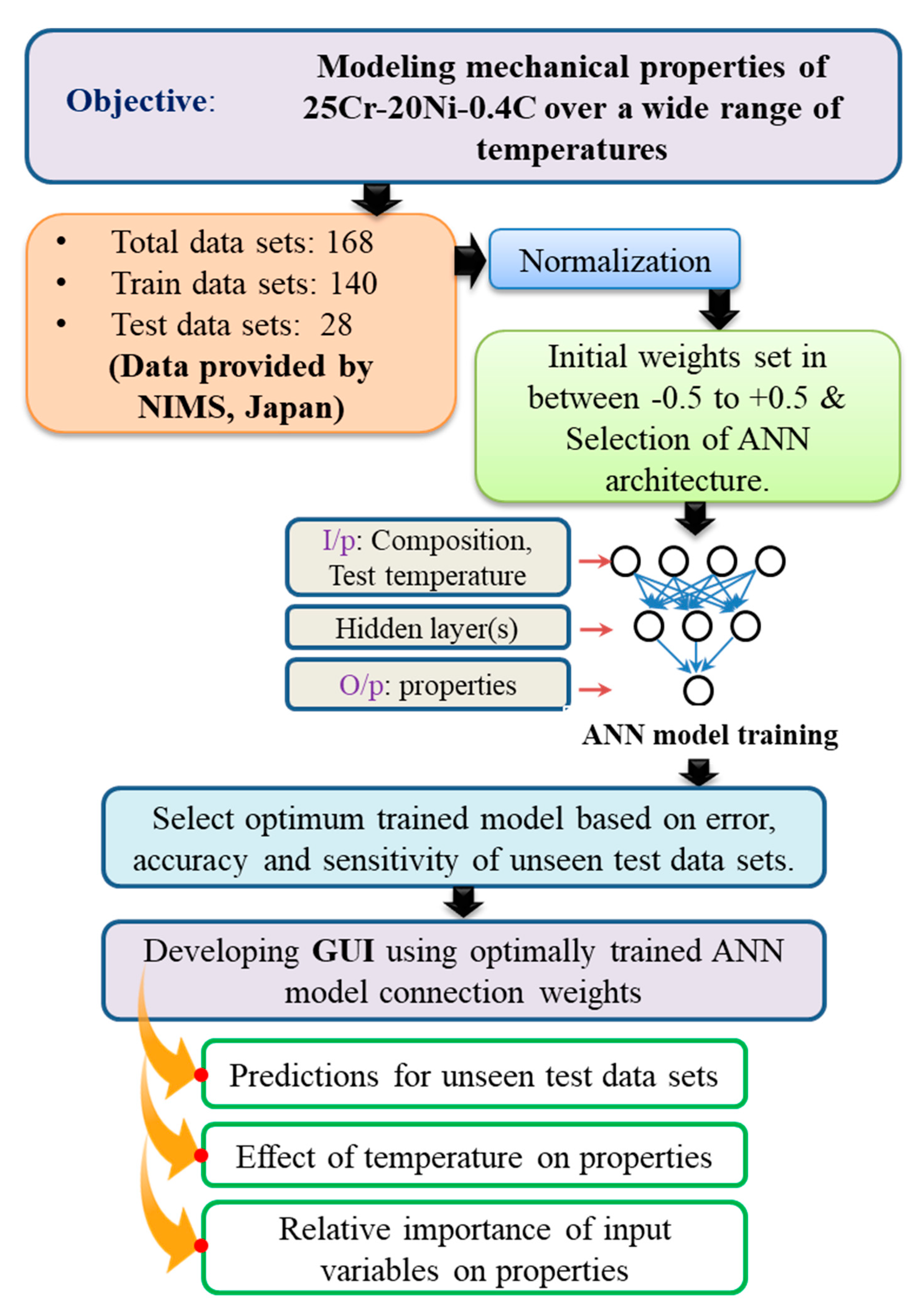
To perform the model training, the entire experimental database was divided into training and testing datasets. Using the training datasets, the optimum architecture of the model was obtained with an appropriate number of hidden neurons and layers, momentum rate, learning rate and number iterations. The training was accompanied in such a manner that the MSE and Etr error values should attain a minimum. The necessary steps that are involved during model training listed are as follows: (i) Selection of hidden layers and neurons, (ii) selection of momentum term and learning rate and (iii) selection of a number of iterations. A detailed flow chart of the present investigation is schematically represented in Figure 1.

Figure 1.
Flow chart describing the various tasks and procedures followed in the present work.
4. Results and Discussion
4.1. Optimization of Model Parameters
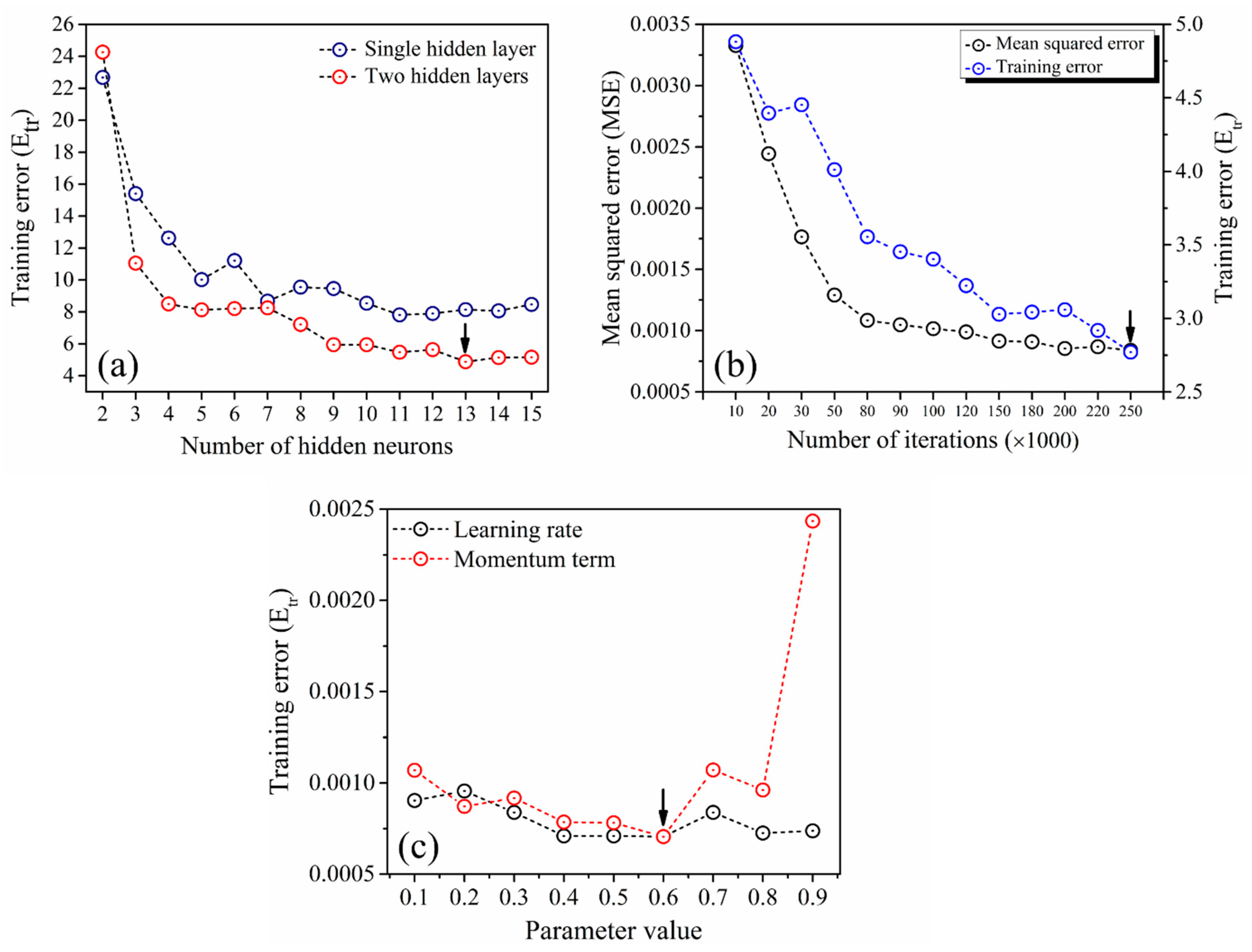
Initially, the ANN model was trained with single and double hidden layers by varying the hidden neurons from two to 15 in each layer. Figure 2a illustrates the change in Etr with hidden neurons in single as well as two hidden layers. From the figure, it is clear that the Etr values of total datasets are gradually decreasing with increasing hidden neurons. As compared with a single hidden layer, training with two hidden layers shows a significant decrease in error values. Within two hidden layers, the minimum error value of both MSE and Etr was noticed at 13 hidden neurons. Hence, the model with two hidden layers containing 13 hidden neurons was considered for further model training. On the other hand, the model was trained with a various number of iterations starting from 10,000 to 250,000. Variation in MSE and Etr as a function of iterations is illustrated in Figure 2b. Both error values were gradually decreased with increasing the number of iterations. Finally, the model with 250,000 iterations reveals the minimum error values, as indicated in Figure 2b. Further training involves the optimization of the model parameters, such as the momentum term (α) and the learning rate (η). Figure 2c shows the decreasing Etr with an increase in momentum term, whereas the higher values of learning rate results in noticeable increment in Etr due to the overtraining of the model. Finally, optimum values of the momentum term and learning rate preferred was 0.6.

Figure 2.
Change in output error a function of (a) hidden layers and neurons, (b) iterations and (c) learning rate and momentum term, respectively.
Hence, after testing several combinations of ANN architecture, the more suitable architecture was obtained with two hidden layers consists of 13 hidden neurons in each layer, with a learning rate of 0.6, the momentum term of 0.6 after 250,000 iterations.
4.2. Weights Distribution during Training
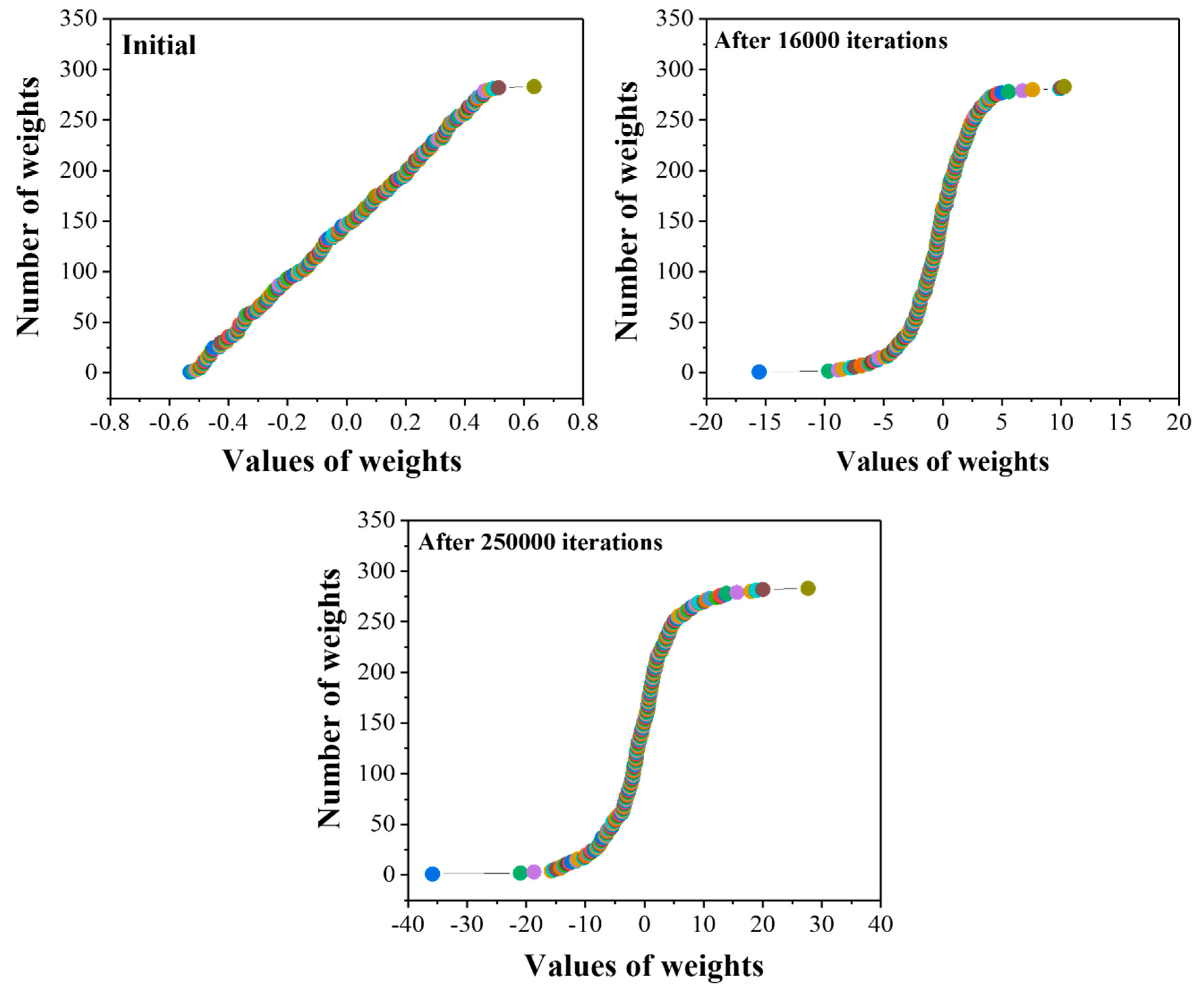
The sensitivity of the trained network with 13-13-4 architecture was improved by a sigmoid transfer or activation function. The transfer function is the main power for the neural networks, which helps to handle the non-linearities. The choice of transfer function strongly influences the complexity and performance of neural networks. Figure 3 represents the weights distribution and the behavior of the sigmoid transfer curve with the function of iterations. From the figure, it is clear that initially (at 0 iterations) the weights distributed linearly within values of −0.6 and 0.6. With an increasing number of iterations, from 0 to 16,000, the curve takes the S-shape with improved weight distribution from −15 to 15. Finally, with optimum iteration values (250,000), the weights were well distributed, ranging from −40 to 40. The well-distributed weights help to correlate the complex relationship between the inputs and output variables, which helps to attain reasonable predictions.
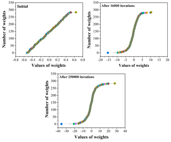
Figure 3.
The distribution of weights as a function of iterations.
4.3. Performance of the Optimum Model
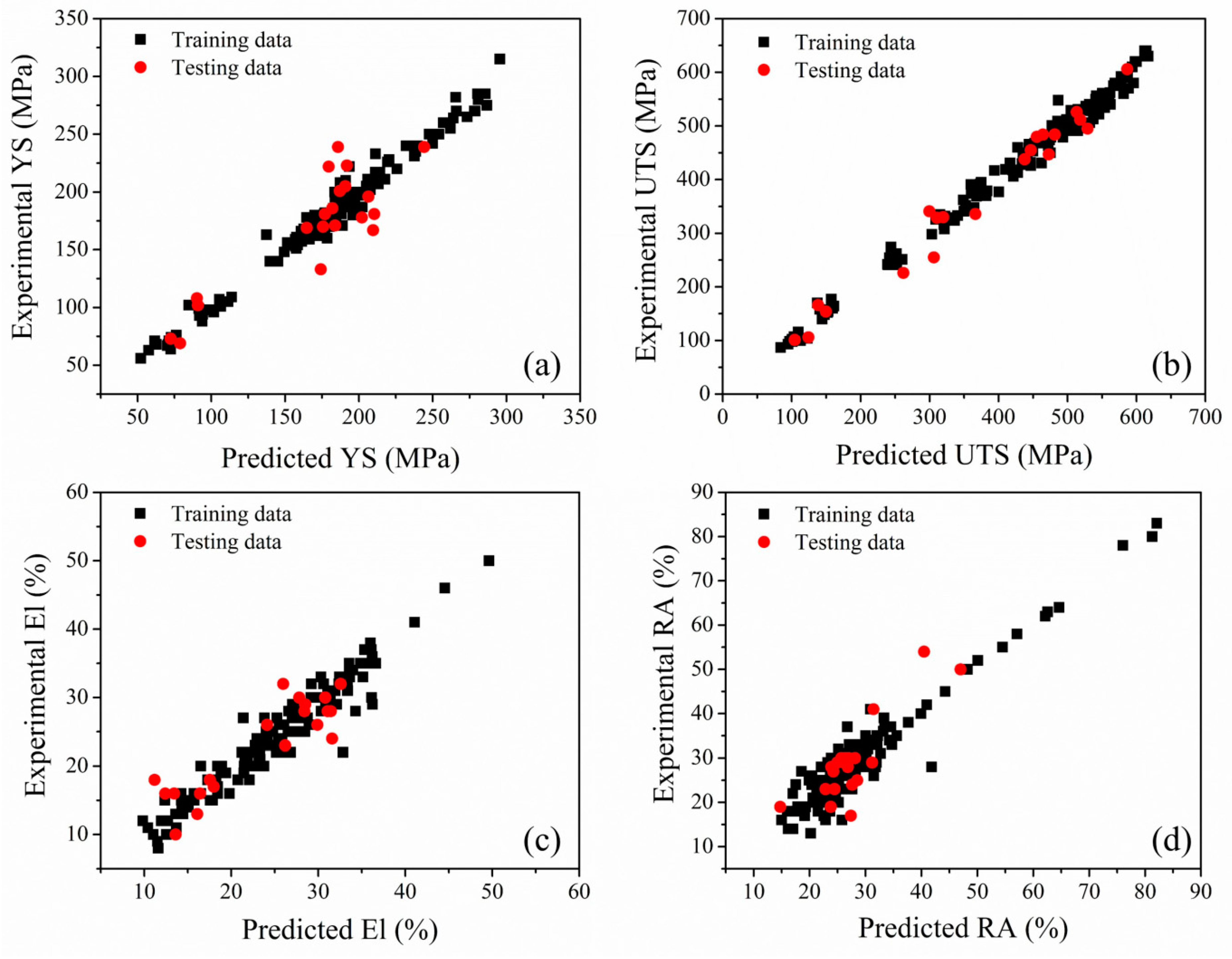
An accurate ANN model is required to generalize the relationships between inputs and outputs for conditions other than those in which it was trained. Since the training and testing data both influence the construction and performance of the algorithms. Hence, the unseen (i.e., previously unemployed datasets during model development) test data were used to assess the ANN model performance. The measured and predicted properties of both training and test datasets of 25Cr-20Ni-0.4C steels are shown in Figure 4. As seen, the ANN models can capture the relationships of mechanical properties with composition and temperature, with the average accuracy of 97% and 89.25% for training and unseen test datasets, respectively. Hence, the present model was capable of predicting the mechanical behavior of the 25Cr-20Ni-0.4C steels as a function of composition and service temperature with sufficient accuracy.
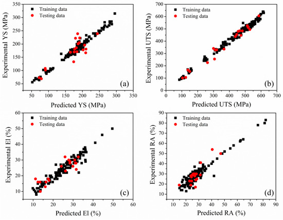
Figure 4.
The ability of the neural network model to predict the mechanical properties of 25Cr-20Ni-0.4C steels: (a) YS, (b) UTS, (c) % El and (d) % RA of the training and test datasets.
4.4. Model Predictions: Effect of Service Temperature on Mechanical Properties
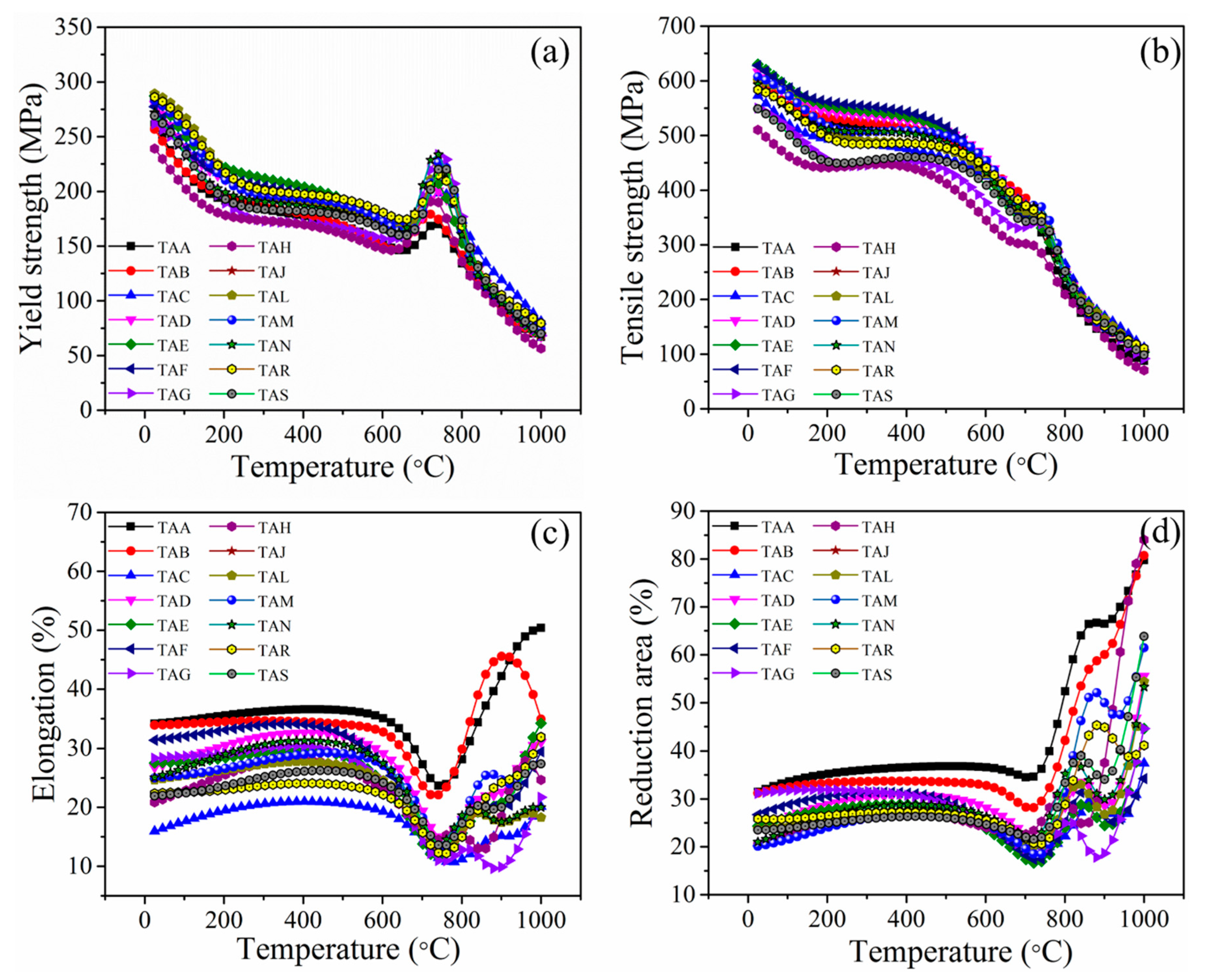
The usefulness of the developed model is not limited to only prediction of unseen test data. The experimental mechanical properties of the steels were available at service temperatures in the steps of 100 °C from room temperature to 1000 °C. Conducting experiments at a higher temperature is expensive. By performing a sensitivity analysis on the developed model [17,18], we simulated the effect of service temperature at minute intervals of temperature on mechanical properties. The estimated tensile properties of 25Cr-20Ni-0.4C steels (TAA–TAS) over a wide range, of 25 to 1000 °C, are illustrated in Figure 5. From the figure, it is noticed that with an increase in temperature from 25 to 1000 °C, the YS as well as UTS of all steels (TAA–TAS), gradually decreases, as shown in Figure 5a,b, respectively. Over 750 °C, the strength of the steels decreased, and the ductility was increased as expected (Figure 5c,d). This predicted phenomenon demonstrates a well-known behavior in engineering materials. Surprisingly, we observed the unexpected increment in YS and respective decrement in % El around the temperatures of 680 to 750 °C for all the steels. In this search space, the experimental data were available only at a temperature of 700 °C. The increase in strength happens at the expense of ductility. However, after thoroughly examining the published literature, we found that the predictions are in accord with the reports of L. Gardener [19] and J. A. Horak [20]. The simulated behavior maps the relationship between the output properties well in the entire predictive range, which is not supplied to the model. Hence, the model predictions revealed an excellent agreement with the practical point of view.
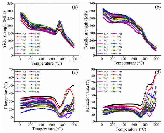
Figure 5.
Effect of service temperature on tensile properties of 25Cr-20Ni-04.C steels: (a) YS, (b) UTS, (c) % El and (d) % RA.
4.5. Model Predictions: Relative Importance Index of Composition on Properties at Various Service Temperatures
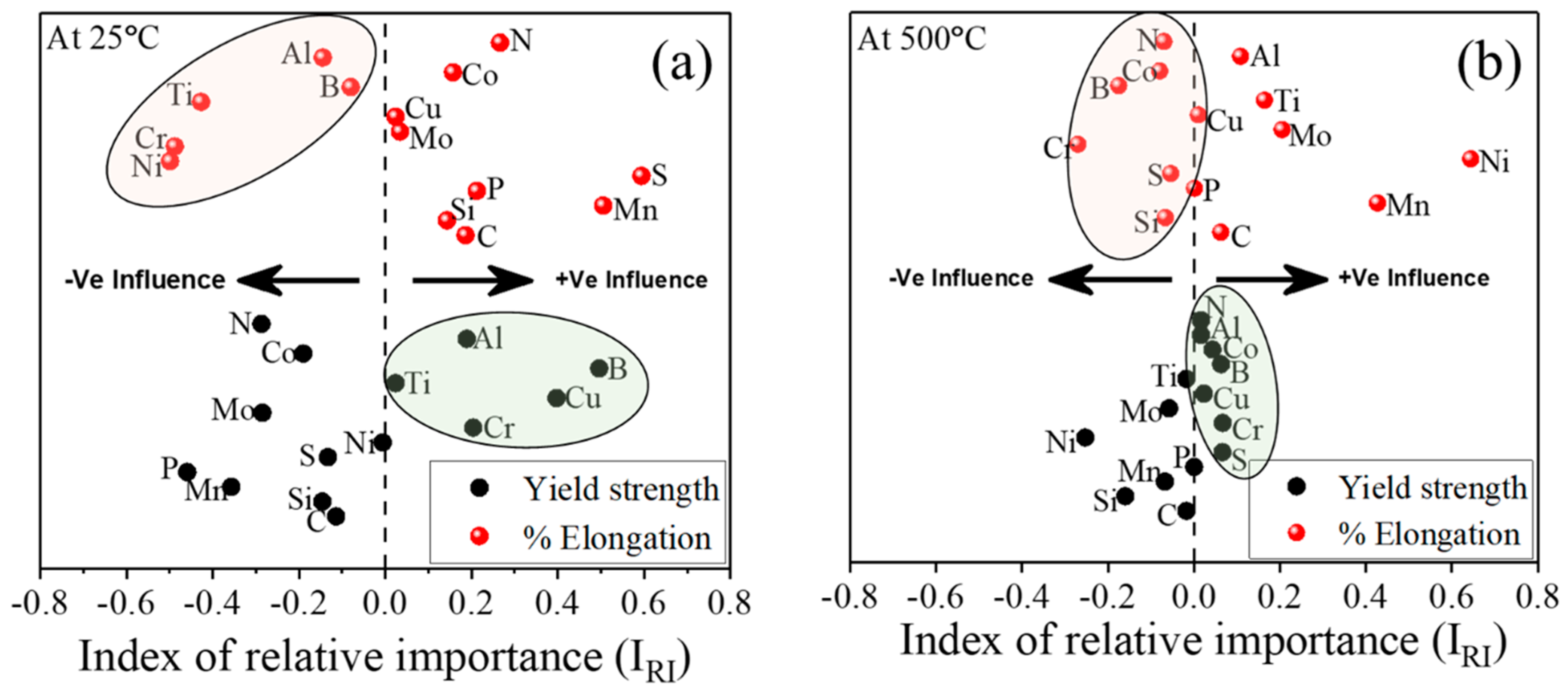
We estimated the influence of alloying elements on YS and % El of 25Cr-20Ni-0.4C steels with the help of the index of relative importance [17,21]. Figure 6 shows the influence of alloying elements on YS and % El of TAA steel at 25 and 500 °C temperatures. At 25 °C, the B, Cr, Cu, Al, and Ti elements show a positive influence on YS. Whereas the same elements exhibit a negative effect on % El (Figure 6a). At 500 °C, the solid solution strengtheners, such as Al, Co, Cu, B and Cr, are favorable for contributing the strength properties, and the same elements are responsible for ductility decrement, as illustrated in Figure 6b. The perceived relative significance of alloying elements may not follow the exact experimental trend; however, the developed model instead helps to understand the significance of alloy composition on properties by recognizing the property trend present in the engineering materials. Likewise, one can determine the significance of alloying elements on the properties of 25Cr-20Ni-0.4C steels within the given range of temperatures using the developed model.
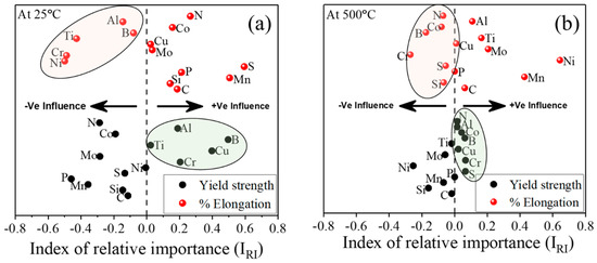
Figure 6.
Significant importance of various alloying elements on YS and % El of TAA steel at (a) 25 °C and (b) 500 °C.
4.6. Design of User-Friendly Graphical User Interface
User-friendly graphical user interface (GUI) of the ANN model is designed to allow the users to interact on the specific task based on the requirement. Within the predictive range of input variables shown in Table S1 (supplementary data), there is an infinite combination of alloys, and experimental conditions are possible. We created a virtual 25Cr-20Ni-0.4C steel with the mean values of the database and estimated the mechanical properties of the steels, as shown in Figure 7. The predicted properties are within the range of the experimental properties. Hence the model will help to predict any combination of input parameters with good accuracy. The developed GUI helps the user to study the accuracy of the developed model and the impact of preferred variables on properties by keeping other variables at specific values by performing sensitivity analysis.
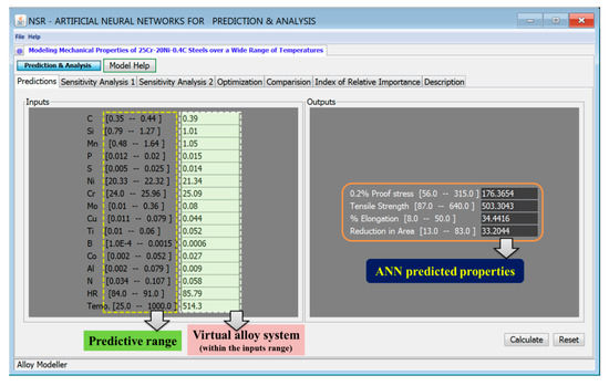
Figure 7.
The screenshot of the ANN model shows the prediction of mechanical properties of a virtual 25Cr-20Ni-0.4C steel by using mean values of all input variables. Within the predictive range of the inputs, there are millions of combinations of experiments possible, of which the model can predict with reasonable accuracy.
5. Conclusions
In conclusion, the present ANN model has a good prediction accuracy for training and unseen testing data sets (an average of 97% and 89.25%, respectively), and it can help to predict the mechanical properties over a predictive range of steels composition as well as the wide range of temperature (25–1000 °C). A standalone ANN software was developed at a negligible computational cost to estimate the mechanical behavior at the minute intervals of the service temperature of 25Cr-20N-0.4C steels. It will save a lot of resources required for the experimentation to determine the mechanical properties. The index of relative importance method was able to identify the individual impact of input variables on the mechanical properties. The model was able to simulate new virtual alloys and the estimated results can provide considerable knowledge to guide actual experiments. Finally, the graphical user interface can help users to access and understand the model easily.
Supplementary Materials
The following are available online at https://www.mdpi.com/2075-4701/10/2/256/s1, Table S1: Chemical composition (mass percent) of various 25Cr-20Ni-0.4C steel tubes, Table S2: Yield strength and ultimate tensile strength of 25Cr-20Ni-0.4C steels at different temperatures. (Note: Bold letters marked with * indicate data sets used for testing), Table S3: The % Elongation and % Reduction of area of 25Cr-20Ni-0.4C steel tubes at different temperatures. (Note: Bold letters marked with * data sets used for testing).
Author Contributions
Conceptualization: N.S.R.; Investigation: J.H.K., J.-K.H., J.-T.Y.; writing—original draft preparation: P.L.N., A.K.M. and N.S.R.; writing—review and editing: N.S.R., C.H.P.; Supervision: N.S.R. and J.-T.Y. All authors have read and agreed to the published version of the manuscript.
Acknowledgments
NSR acknowledges YSJ-SAR and YKK for motivation and model development, respectively. This work was supported by the Fundamental Research Program of the Korea Institute of Materials Science (PNK6230) and Ministry of Trade, Industry and Energy (10081334).
Conflicts of Interest
The authors declare no conflicts of interest.
References
- Sucre, Y.R.; Vogt, J.B.; Iost, A.; Najjar, D.; Chumlyakov, Y.I. Mechanical properties of austenitic stainless steel single crystals: Influence of nitrogen and hydrogen content. Metall. Mater. Trans. A 2000, 31, 153–161. [Google Scholar] [CrossRef]
- McGuire, M.F. Austenitic stainless steels. In Encyclopedia of Materials: Science and Technology; Buschow, K.H.J., Cahn, R.W., Flemings, M.C., Ilschner, B., Kramer, E.J., Mahajan, S., Veyssière, P., Eds.; Elsevier: Oxford, UK, 2001; Volume 4, pp. 406–410. [Google Scholar]
- Zhou, Y.; Liu, Y.; Zhou, X.; Liu, C.; Yu, J.; Huang, Y.; Li, H.; Li, W. Precipitation and hot deformation behavior of austenitic heat-resistant steels: A review. J. Mater. Sci. Technol. 2017, 33, 1448–1456. [Google Scholar] [CrossRef]
- Vujic, S.; Sandström, R.; Sommitsch, C. Precipitation evolution and creep strength modelling of 25Cr20NiNbN austenitic steel. Mater. High Temp. 2015, 32, 607–618. [Google Scholar] [CrossRef]
- Wachter, O.; Brümmer, G. Experiences with austenitic steels in boiling water reactors. Nucl. Eng. Des. 1997, 168, 35–52. [Google Scholar] [CrossRef]
- Moteshakker, A.; Danaee, I. Microstructure and Corrosion Resistance of Dissimilar Weld-Joints between Duplex Stainless Steel 2205 and Austenitic Stainless Steel 316L. J. Mater. Sci. Technol. 2016, 32, 282–290. [Google Scholar] [CrossRef]
- Sun, H.; Sun, Y.; Zhang, R.; Wang, M.; Tang, R.; Zhou, Z. Hot deformation behavior and microstructural evolution of a modified 310 austenitic steel. Mater. Des. 2014, 64, 374–380. [Google Scholar] [CrossRef]
- Steinhauser, M.O.; Hiermaier, S. A review of computational methods in materials science: examples from shock-wave and polymer physics. Int. J. Mol. Sci. 2009, 10, 5135–5216. [Google Scholar] [CrossRef] [PubMed]
- Sourmail, T.; Bhadeshia, H.K.D.H.; MacKay, D.J.C. Neural network model of creep strength of austenitic stainless steels. Mater. Sci. Tech. 2002, 18, 655–663. [Google Scholar] [CrossRef]
- Cui, Y.; Sauzay, M.; Caes, C.; Bonnaillie, P.; Arnal, B.; Cabet, C.; Blat-Yrieix, M.; Dubiez-Legoff, S. Modeling and experimental study of long term creep damage in austenitic stainless steels. Eng. Fail. Anal. 2015, 58, 452–464. [Google Scholar] [CrossRef]
- Feng, W.; Yang, S. Thermomechanical processing optimization for 304 austenitic stainless steel using artificial neural network and genetic algorithm. Appl. Phys. A 2016, 122, 1018. [Google Scholar] [CrossRef]
- Reddy, N.S.; Krishnaiah, J.; Hong, S.-G.; Lee, J.S. Modeling medium carbon steels by using artificial neural networks. Mater. Sci. Eng. A 2009, 508, 93–105. [Google Scholar] [CrossRef]
- Narayana, P.L.; Kim, S.-W.; Hong, J.-K.; Reddy, N.S.; Yeom, J.-T. Estimation of Transformation Temperatures in Ti–Ni–Pd Shape Memory Alloys. Met. Mater. Int. 2018, 24, 919–925. [Google Scholar] [CrossRef]
- Reddy, N.S.; Rao, A.K.P.; Chakraborty, M.; Murty, B.S. Prediction of grain size of Al–7Si Alloy by neural networks. Mater. Sci. Eng. A 2005, 391, 131–140. [Google Scholar] [CrossRef]
- Lippman, R. An introduction to computing with neural nets. IEEE ASSP Mag. 1987, 4, 4–22. [Google Scholar] [CrossRef]
- Hassoun, M.H. Fundamentals of artificial neural networks. In Proceedings of the IEEE; MIT Press: New York, NY, USA, 1995. [Google Scholar]
- Reddy, N.S.; Panigrahi, B.B.; Ho, C.M.; Kim, J.H.; Lee, C.S. Artificial neural network modeling on the relative importance of alloying elements and heat treatment temperature to the stability of α and β phase in titanium alloys. Comput. Mater. Sci. 2015, 107, 175–183. [Google Scholar] [CrossRef]
- Reddy, N.S.; Lee, C.S.; Kim, J.H.; Semiatin, S.L. Determination of the beta-approach curve and beta-transus temperature for titanium alloys using sensitivity analysis of a trained neural network. Mater. Sci. Eng. A 2006, 434, 218–226. [Google Scholar] [CrossRef]
- Gardner, L.; Insausti, A.; Ng, K.; Ashraf, M. Elevated temperature material properties of stainless steel alloys. J. Constr. Steel Res. 2010, 66, 634–647. [Google Scholar] [CrossRef]
- Horak, J.; Sikka, V.; Raske, D. Review of mechanical properties and microstructures of Types 304 and 316 stainless steel after long-term aging. In Proceedings of the IAEA Specialists on Mechanical Properties of Structural Materials, Chester, UK, 10 October 1983. [Google Scholar]
- Sadan, M.K.; Ahn, H.-J.; Chauhan, G.S.; Reddy, N.S. Quantitative estimation of poly(methyl methacrylate) nano-fiber membrane diameter by artificial neural networks. Eur. Polym. J. 2016, 74, 91–100. [Google Scholar] [CrossRef]
© 2020 by the authors. Licensee MDPI, Basel, Switzerland. This article is an open access article distributed under the terms and conditions of the Creative Commons Attribution (CC BY) license (http://creativecommons.org/licenses/by/4.0/).

