Non-Destructive Micromagnetic Determination of Hardness and Case Hardening Depth Using Linear Regression Analysis and Artificial Neural Networks


1
Leibniz-Institute for Materials Engineering—IWT, 28359 Bremen, Germany
2
MAPEX Center for Materials and Processes, University of Bremen, 28359 Bremen, Germany
*
Author to whom correspondence should be addressed.
Metals 2021, 11(1), 18; https://doi.org/10.3390/met11010018
Submission received: 20 November 2020
/
Revised: 19 December 2020
/
Accepted: 19 December 2020
/
Published: 24 December 2020
(This article belongs to the Special Issue Advances in Design by Metallic Materials: Synthesis, Characterization, Simulation and Applications)
Abstract
:Non-destructive determination of workpiece properties after heat treatment is of great interest in the context of quality control in production but also for prevention of damage in subsequent grinding process. Micromagnetic methods offer good possibilities, but must first be calibrated with reference analyses on known states. This work compares the accuracy and reliability of different calibration methods for non-destructive evaluation of carburizing depth and surface hardness of carburized steel. Linear regression analysis is used in comparison with new methods based on artificial neural networks. The comparison shows a slight advantage of neural network method and potential for further optimization of both approaches. The quality of the results can be influenced, among others, by the number of teaching steps for the neural network, whereas more teaching steps does not always lead to an improvement of accuracy for conditions not included in the initial calibration.
1. Introduction
The heat treatment state of a case-hardened steel workpiece especially surface hardness and case hardening depth, which also often correlates with the surface oxidation depth, are important properties for the final service properties of high-performance parts, which have to be continuously controlled in industrial production. Further, these surface properties influence the grindability of the components as well as the micromagnetic detectability of grinding damages [1,2]. Therefore, the knowledge of these properties can allow determining optimal grinding parameters as a function of the component’s initial state and can enable a reliable in-process micromagnetic monitoring of the grinding processes [3]. Besides the known destructive testing methods which are precise but time-consuming, the heat treatment condition can also be assessed non-destructively using micromagnetic methods such as Barkhausen noise analysis or the 3MA-technique [4].
Using micromagnetic methods, hardness is in most cases determined by calibration using linear regression [4,5]. To determine the case hardening depth by means of Barkhausen noise analysis, several additional approaches based on the different properties of soft core and hard surface layer exist. For example, Send et al. observed additional peaks and asymmetries of the Barkhausen peak generated by the hardened case that could be described with different parameters and correlated with the case hardening depth [6]. In [7] Santa-aho et al. employed sweeps of the magnetization voltage to determine the maximum slope of Barkhausen noise for two magnetizing frequencies (and therefore different penetration depth) and correlated the ratio with the case hardening depth. The 3MA-technique combines four micromagnetic methods with different penetration depth. Besides the Barkhausen noise, it includes, among others, the method of harmonic analysis of the tangential magnetic field. Here, the case hardening could be correlated to the frequency limit at which the distortion factor is near to an asymptote [8]. Further influences of case depth on the frequency characteristics of various micromagnetic signals were observed in [9], but could not be fully explained.
In [10] and [11], among others, artificial neural networks were used to determine hardness from hysteresis loop and eddy current measurement respectively Barkhausen noise and tangential magnetic field analysis. Besides hardness, Liu et al. determined residual stresses and case depth from a combination of Barkhausen noise, tangential magnetic field, and hysteresis measurement by use of artificial neural networks [12]. Sorsa et al. compared the suitability of linear regression, artificial neural networks, and fuzzy models for determination of residual stresses from Barkhausen noise measurements. They identified better performance indices RMSE (root mean square error) and R2 (coefficient of determination) for artificial neural networks than for linear regression but also pointed out an advantage of linear regression. Indeed, this method has a low risk of overfitting and is therefore well suited for small calibration data sets and extrapolation. To achieve good regression results, a preselection of significant features was performed, as a too high number of inputs led to overfitting of the network [13]. Furthermore, in [10] only a single digit number of measured variables was used for hardness determination. Criterion for the selection was the ratio of standard deviation and mean value. An improvement of the performance could be achieved by additional measured variables. The influence of the volume of the data set is described in [11]. An extension of the calibration data set leads to decrease of the standard error. For the given example of 17 measurement points over a Jominy sample with three hardness zones, the standard error starting with nine data points in calibration was below 5% of the maximum hardness.
Further actual studies handle with the correlation of magnetic properties with hardness, residual stresses, and other properties. In general, decreasing hardness [14] and increasing (tensile) residual stresses [15,16] led to an increase in the Barkhausen noise level. While increase of Barkhausen noise with residual stresses in some cases is not linear due to poor magnetization, the averaged permeability derived from hysteresis loop shows a much better linear correlation [16]. Other works describe linear increase with rising tensile stresses for Barkhausen noise as well as permeability [17,18]. Besides the maximum and average values of Barkhausen noise and permeability, various other measured variables are determined from the raw signal depending on the measuring device. The coercivity develops roughly opposite to the Barkhausen noise or permeability level and correlates well with the hardness as well as residual stresses [17,19]. Peak width decreases with increasing tensile stresses. Remanence decreases with increasing hardness [19].
The aim of the present work is the non-destructive evaluation of the heat treatment state of case-hardened steel workpieces by means of micromagnetic 3MA-measurements with variation of magnetization and analysis frequencies. Instead of the first mentioned often very complex approaches for the evaluation of frequency sweeps, different calibration strategies were developed. In order to use the possibilities of frequency-dependent analyses for the determination of gradient properties, different from previous works, a large number of measured variables were included. After calibration using samples with known properties, these can simply be applied to the following measurements. For this purpose a comparison of classical regression analysis and calibration using artificial neural networks was carried out. A sample set with two-stage variation of three variables and two samples per state was prepared for calibration and analysis. Special attention was therefore paid to the challenges of—compared to number of measured variables and influences on heat treatment state—small calibration data sets. Standard errors of calibration data and unknown test data were compared. Possible influences of different parameters on the quality of the result were evaluated and compared.
1.1. Micromagnetic Measurements and Data Evaluation
The 3MA-II-technology (Micromagnetic Multiparametric Microstructure- and Stress-Analysis) developed by Fraunhofer Institute for Nondestructive Testing (IZFP) combines the four micromagnetic methods Barkhausen Noise (BN), Harmonic Analysis of the tangential magnetic field strength (HA), Incremental permeability (IP), and multi-frequency Eddy Current analysis (EC). Together these methods provide 41 measured variables with different sensitivity to microstructure and stress state. Due to the frequency ranges the methods have different analyzing depths. The combination of measuring parameters allows a separation of different influences such as residual stresses and hardness as well as the compensation of disturbances [20]. An additional software tool, the so-called sweep module, enables the automatized and fast variation of measurement parameters such as frequency and magnetization amplitude [4,9].
BN results from the stepwise shift of Bloch walls, separating magnetic domains, during magnetization of ferromagnetic materials. If no further Bloch wall shifts are possible, the domains are aligned in direction of the field by rotation processes as the magnetization continues to increase [21]. In this region the magnetic hysteresis loop, becomes flatter until it becomes horizontal in the saturation state [22]. A schematical hysteresis curve is shown in Figure 1. After amplifying, filtering, and rectifying the recorded BN signal, its envelope or profile curve is displayed above the magnetic field strength . The shape of the hysteresis curve, the profile curve, and thus the characteristic parameters are influenced by the microstructure, the mechanical properties, and residual stress state [9,20]. Mechanically hard materials are magnetically hard with high coercivity HCM and low remanence MR and maximum Barkhausen noise amplitude MMAX because Bloch wall shifts interact analogous to dislocation movements. Other measured variables are the averaged amplitude over one magnetization cycle MMEAN and the curve width at 25%, 50%, and 75% of MMAX called DH25M, DH50M, and DH75M, respectively. Compressive stresses cause a high coercivity and low amplitude, tensile stresses a low coercivity and high amplitude [4,23,24,25].
Depending on the frequency, different depth ranges can be investigated. According to (1), the exponential damping function results in the penetration depth at which the amplitude of the magnetic field is still of the intensity at the surface. Thereby, the relative permeability and the electrical conductivity are material and heat treatment-dependent parameters [26]. The high-pass frequency of the Barkhausen noise signal can be stepwise varied between no limitation and 1 MHz, and low-pass between 500 kHz and no limitation. Due to the base magnetization frequency between 10 Hz and 1000 Hz, harmonic analysis has the largest possible analyzing depth of the four testing methods with up to several mm probing depth [4]. The analyzing depth of the Barkhausen noise, depending on the analyzing frequency range, is in a range from about 10 µm to a few 100 µm [9]. In this particular case of hardened surface layers, an analyzing depth of up to 50 µm can be assumed [27]. The analyzing depth of the incremental permeability is in a similar range [9]. Depending on the set frequencies the eddy current analysis can reach large range of depth from about 10 µm to few hundred microns.
In the harmonic analysis of the tangential magnetic field strength, the sample volume to be examined similar to Barkhausen noise analysis is magnetized by a sinusoidal alternating field. The development of the tangential field strength during the hysteresis loop is recorded by a Hall probe and processed by Fourier analysis. In this way, the odd higher harmonics can be determined. Measured variables generated from this are the amplitudes A3…7 and phases P3…7 of the harmonics, the distortion factor K(2), the sum of all upper harmonics UHS, the coercive field strength HCO of the harmonic analysis (increases with hardness), the harmonic content of the magnetic field strength at zero crossing , and the final stage voltage of the electromagnet . Soft magnetic materials generally lead to a high distortion factor and vice versa [4].
To determine the incremental permeability , the hysteresis loop is superimposed by a further higher-frequency hysteresis loop. The signal picked up in this process corresponds to the incremental permeability, which is determined by alternating field strength changes at various points in the hysteresis loop, which would require an enormous amount of time in practice. The incremental permeability µ plotted against the magnetic field strength results in a similar curve shape as the Barkhausen noise M and the determination of the measured variables is carried out in the same way. While the Barkhausen noise is based on irreversible Bloch wall jumps, the incremental permeability depicts reversible processes [8].
In eddy current analysis, a high-frequency alternating weak magnetic field is generated. This primary field generates electric eddy currents, which are accompanied by a secondary field in the opposite direction to the primary field. A receiver coil measures the magnetic field as induced voltage. The eddy currents and thus the induced voltage are influenced by both the conductivity and permeability of the sample. The 3MA-II technology allows the simultaneous use of four eddy current frequencies. Real parts Re1…4 and imaginary parts Im1…4 as well as magnitude Mag1…4 and phase angle Ph1…4 of the voltage are output as measured variables [4].
1.2. Regression Analysis
For quantitative determination of a target quantity (e.g., hardness) it is necessary to find a calibration function which describes the relationship between target quantity and variables. Because the theoretical calculation of this relationship with physical models is possible at least for simple materials, 3MA is usually calibrated based on empirical data [4]. For this purpose, the target values are determined with a reference method (e.g., hardness testing) and stored in a database together with the micromagnetic measurements to analyze correlations by use of regression analysis or pattern recognition. Possible terms of the regression are the measurement parameters of 3MA as measured, their squares and square roots. The coefficients are determined by method of least squared errors [4,8,28]. Measures for the goodness of a regression are the coefficient of determination R2 and the root mean square error RMSE [28].
An adjustment of the regression algorithm makes it possible to minimize the effect of drifts of measured variables on the regression result. This is of special interest for low-frequency and systematic stochastic errors, for example due to ageing or wear of the sensor, that cannot be reduced by a larger number of measurements in the calculation of averages. The range of values gives the minimum and maximum value of a partial expression in the calibration data set.
(3) gives the modulation and (4) the 1% error effect. If the measured value changes by 1% of the regression result changes by the value . The larger the error effect, the greater the reproducibility of the measured variables. The calibration wizard of the 3MA-MMS software gives the opportunity to choose the highest tolerated . This limitation reduces the possible expressions to those that fulfill the condition. A too strong limitation of the 1% error effect leads also to a decreasing coefficient of determination and a rising standard error RMSE, as the remaining terms have not only a small error effect but only a small effect at all [8].
1.3. Artificial Neural Networks
Artificial neural network (ANNs) consist of several interconnected processing units called neurons, which can be divided in input, hidden, and output units and are arranged in layers (Figure 2a). The input units of the first layer distribute the components of the net input vector to the units of the second layer. The second till second last layer are hidden layers [29,30]. Every neuron consists of data collection (neuron input), processing, and sending results (neuron output), as shown in Figure 2b. To understand the process it is important to differentiate between the net-input or -output (Figure 2a) and the neuron-input or -output (Figure 2b). The weights of the links control the effect of the inputs on a neuron. They are changed during training of the ANN to optimize the relation of input and output and carry the information of the ANN. The weighted neuron inputs are summed and the transfer function determines the neuron output. There are several possible linear and nonlinear transfer functions to choose when constructing the network [31,32].
For training of an ANN (i.e., optimization of the weights) there are three general learning strategies, the supervised, unsupervised, and reinforcement learning. For supervised learning, the training set consists of (net) inputs and the related outputs. In unsupervised learning, only (net) inputs are given and the network learns without intervention of the trainer. Reinforcement learning means that the trainer only indicates whether the output of the network is correct or not. To evaluate the quality of the trained network in a test phase with unknown input, the pattern set is split up into teaching set and test set before teaching phase [29]. Furthermore it is necessary to normalize the net input and output values into the range 0–1 before teaching to get similar ranges for all variables [31,32].
A commonly used training algorithm for nets with input layer, output layer, and hidden layers is the backpropagation algorithm. Every teaching step consists of a forward pass and a backward pass. The forward pass starts with the input layer, the output of every unit is transmitted to the next layer till the output layer is reached. The estimated net outputs are compared with the correct outputs . Through the backward pass the differences are stepwise given back from the output layer to the first hidden layer and the weights are dated up to minimize the error of the next teaching step [31,32].
2. Materials and Methods
The sample set consists of 54 discs made from one batch of steel AISI 4820 (DIN 18CrNiMo7-6) with a diameter of 68 mm and a thickness of 20 mm. The chemical composition of the steel batch was analyzed with an optical emission spectrometer ARL 3460 (Thermo Fisher Scientific, Waltham, MA, USA) and is given in Table 1.
The samples were gas carburized and oil quenched in 27 variations given in Table 2. The heat treatment was performed in a chamber furnace (Aichelin Holding GmbH, Mödling, Austria). Details for case hardening are shown in Figure 3 and Table 3. After oil quenching, the samples were tempered for two hours at the temperatures given in Table 2.
Surface hardness and carburization depth, as an approximation of the case hardening depth (CHD), were determined at smaller coupon samples treated in the same heat treatment batches as the samples for the investigations. Surface hardness was measured according to Vickers with a LV-700AT (LECO Instrumente GmbH, Mönchengladbach, Germany) with a test load of 9.807 N (HV1). To determine the carburization depth, carbon depth profiles were recorded using spark optical emission spectroscopy (ARL 3460, Thermo Fisher Scientific, Waltham, MA, USA). The carburization depth is defined as the depth with a carbon content of 0.3 wt. %.
Micromagnetic measurements were performed with a 3MA-II device from Fraunhofer IZFP, Saarbrücken, Germany and a standard sensor with convex pole shoes and spring-mounted transducer unit. The measurement settings are given in Table 4. The magnetization frequency, high-pass frequency, and eddy current frequency of the incremental permeability IP were varied with the sweep module to record a total of 425 measurement quantities with different analyzing depths. All samples were measured ten times at one position of the circumference with magnetization in tangential direction.
After a first check of the data set and removal of samples with obvious outliers, calibration was carried out using the calibration module of the 3MA software and also by artificial neural networks. For calibration with linear regression analysis, the data obtained with magnetization frequency of 20 Hz were removed from the data set. For this frequency, instability of the magnetization meant that several measurement parameters of the IP could not be determined consistently. As this would reduce the information content of the data set, as only complete measurements with all parameters are used for regression, the magnetization frequency was removed from all data sets.
Linear regression with the “calibration wizard” of 3MA-software (Fraunhofer IZFP, Saarbrücken, Germany) [4,8] was carried out with carburization depth and hardness as target values. The maximum number of terms of the polynomial was set to 10. As mentioned in chapter 1, the limitation of the maximum error effect leads to an improvement especially for low-frequency stochastic errors (e.g., due to wear/ageing of the sensor). Nevertheless the maximum error effect was varied here to identify possible effects, e.g., in context of deviations due to contact between sensor and sample. Maximum error effect was reduced stepwise to find a setting with reduced error effect without too strong worsening of the regression quality. For both, the unlimited and the optimized error effect, additionally to these of the calibration data set R2 and RMSE of test samples, which were not included in the calibration/training, were evaluated.
When dividing the data set into test and calibration data set, a too small calibration data set would lead to a bad regression result. In contrast, a large calibration data set reduces the test data set and thus the reliability of the control. Therefore, for the maximization of calibration and test data set the autorecognition test described in [8] was used. Each of the samples (10 measurements) is taken out of the calibration data set and used for validation one time. After calibrations with samples, every sample is used for validation one time.
For the artificial neural network analysis, 425 input neurons were employed as well as the same number of hidden neurons and output neurons with carburization depth and hardness as net output. The net was constructed in the software MemBrain [33,34] (free version for non-commercial and educational use, Thomas Jetter, Mainz, Germany). The activation function (transfer function) is a logistic function. The net was taught/trained with backpropagation method over 30 and 60 repetitions of the teaching lesson. Results were evaluated in the same way as described for regression analysis.
To get an idea about advantages and disadvantages with the use of sweeps, additional calibrations were performed with only the measured variables of the standard configuration. Linear regression was performed without limitation of the maximum error effect and network training with 30 repetitions.
3. Results and Discussion
As a result of the heat treatment variations described in Table 2, material states with carburization depth of approximately 0.55 mm, 0.9 mm, and 1.9 mm and surface hardness between 640 HV1 and 760 HV1 were generated. All measured data are presented in Table A1. Figure 4, Figure 5 and Figure 6 show carbon profiles (a), microhardness profiles (b), and cross sections (c) of samples with target case hardening depth of 0.5 mm, 1 mm, and 2 mm. Comparison of the marked Case Hardening Depth (CHD 550), the carburization depth (0.3 wt. % carbon) and the transition between case hardened layer and bulk material in the cross section shows that carburization depth can be used as reliable closely related values to evaluate the CHD.
3.1. Calibration by Use of Regression Analysis
Linear regression of the hardness without limitation of the maximum error effect leads to an error effect of F1 = 9.274 HV1. The determination coefficient of this regression is R2 = 0.8709 and the standard error RMSE = 12.919. Table 5 shows the change of determination coefficient and standard error due to limitation of the error effect. A limitation to F1 = 3 HV1 was chosen as optimum since with a stronger limitation there would be a too strong decrease of the determination coefficient and increase of the standard error.
Micromagnetic determined hardness of the calibration data set plotted over the measured hardness is shown in Figure 7. There is no pronounced difference due to the limitation of the error effect. The plotted data points all represent an averaged value for the 10 micromagnetic measurements per sample and the associated standard deviation. This average is the reason for the difference between the standard errors given in Table 5 and Figure 7.
Figure 8 shows the measured and determined hardness for unknown samples, not included in the calibration (autorecognition test). The standard error is about 50% higher than for the calibration data set shown in Figure 7 and reaches values of 15% of the range of target values. The influence from limitation of the error effect on the result is very low. For later use of the calibration function, it would be more indicated to use the calibration function with reduced F1 values in order to reduce possible effects of sensor ageing or of a change of the sensor.
The terms of the regression are summarized in Table 6. No measured parameters from Eddy Current analysis is part of the calibration function but values from Harmonic Analysis (A3–A7, P3–P7, Vmag, Hco), Barkhausen noise (MMAX, HCM, Mr), and Incremental Permeability (DH25µ, µr) with different frequencies. As the values for the regression analysis are not normalized, the regression coefficients do not allow any conclusion about relevance of the single terms. It is obvious that some measured variables appear with a positive and negative prefix. For example, MMAX is part of the regression result as negative term, what corresponds to the state of the art, but later MMAX2 appears as positive term. HCM2 is part of the result as negative term whereas it typically increases with hardness.
Plotting the hardness over the various measured variables shows the best correlation with the remanence of the incremental permeability measurement (Figure 9). However, no obvious relationship between hardness and the measured variables from Harmonic Analysis could be observed. The different suitability of the measurement methods for determining hardness can be explained by the different penetration depths depending on the frequency. An overview of correlation of different measured variables with hardness and carburization depth is given in Table A2. The comparison with Table 6 and Table 9 shows that not all terms of the regression result are visibly correlated with hardness respectively carburization depth. On the one hand, this indicates that the calibration would be possible also with a lower number of terms. On the other hand, due to variation of surface carbon content, case hardening depth, and tempering temperature, signals are affected by multiple influences. Measured variables with coefficient of determination of more than 0.25 are remanence of Barkhausen noise and incremental permeability which correlate negatively with the hardness and peak width at 25% of the maximum of the incremental permeability. This is consistent with the known general correlations.
To make sure that only relevant measurement parameters are included in calibration the number of possible terms was limited to less than 10 (Table 7). A stronger limitation of the number of regression terms leads to a decrease of the coefficient of determination and an increasing standard error. But at the same time there is a clear decrease of the error effect. Regression with a high number of terms fits very well to the teaching data set but does not necessarily lead to an improvement on the result for unknown test data (exemplary shown for 20, 10, and 6 terms). A limitation of the number of terms thus has a similar effect as the limitation of the maximum error effect. The most important measured value, which is used to calculate hardness with only two terms is the remanence of the incremental permeability µr.
Additionally, a comparison of Figure 9a,b shows no difference in the qualitative evolution for different frequencies. A limitation to fewer frequency variants or a single frequency should therefore be possible without negative effects on the calibration but would reduce the measurement and calibration effort. Furthermore, this is in agreement with the results of previous studies, where calibration was carried out with only few preselected variables.
Similar to the hardness, the measurements were calibrated for carburization depth. Table 8 again shows the regression quality in dependence of the maximum error effect. A maximum error effect of 0.06 mm was chosen as optimum.
Figure 10 shows the carburization depth calculated without (a) limitation of the error effect plotted over the measured carburization depth. For this calibration data set there is a good agreement of measured and calculated values with a standard error of 0.074 mm, what is ~6% of the range of target values. The limitation of the error effect (b) only slightly affects the goodness of the prediction since small increase of RMSE is resulting.
The same calibration types with and without limitation of the error effect in Figure 11 are illustrated for the test data set. The standard errors again are obviously higher than those of the calibration data set but with these are still within an acceptable range of reliability with errors around 10% of the target values. Without taking into account the outlier at 1.87 mm, the RMS is 0.105 mm for only 8% of the range of target values. As for the calibration data set, no pronounced effect due to the limitation of the maximum error effect can be observed, and the standard error increases slightly.
The regression terms for the determination of carburization depth are shown in Table 9. Again, the function contains measured variables from different methods and frequencies. Compared to the hardness determination the importance of Harmonic analysis and low frequencies (larger penetration depth) increases. Measured variables with best coefficient of determination (see Table A2) are K, Hcm, and Hco which all correlate positive with carburization depth. This corresponds to the general relationship that these measured variables increase with hardness.
Again, a stronger limitation of the number of regression terms leads to lower coefficients of determination and lower error effects (Table 10). To calculate the carburization depth of unknown samples, the function with 10 terms gives good results but a limitation on six or eight regression terms could also be used, as a good compromise between the standard error and the maximum error effect. Similar to the observations of Table 9, regression results with six or less terms are based on measured variables from harmonic analysis and the coercivity Hcm (80 Hz).
3.2. Calibration by Use of Artificial Neural Networks
The output of the artificial neural network plotted over the measured hardness is shown in Figure 12 after 30 (a) and 60 (b) iterations of the teaching lesson. The standard error is much lower than after calibration with linear regression and decreases significantly with duplication of the number of teaching lessons. RMSE = 7.1 HV1 after 30 teaching lessons are in the same range as the standard deviation of Vickers hardness measurements so as the RMSE = 3.7 HV1 after 60 lessons.
For the unknown test data (autorecognition test), the standard error between measured hardness and net output is much higher than for the training data (see Figure 13). It is slightly below than after regression analysis but the difference between teaching and test data set is significantly higher. The duplication of the number of training lessons does not lead to pronounced change of the accuracy with a slight increase of the standard error. This illustrates the risk of overfitting. If the network adapts too much to the training data, this is at the expense of the quality of the prediction for unknown test data. For optimization, the number of teaching lessons should therefore be increased stepwise. As the standard error of the training data set continues to decrease or gets towards an asymptote, the standard error of the test data set will rise if the net overfits the training data. With the size of the network, the ability to fit complex solutions increases as well as the risk of overfitting [35]. Therefore, besides the number of training steps, the number of input variables also offers optimization potential.
After doubling the training steps for calculation of hardness no improvement of the results was resulting. Figure 14 shows therefore only the network output for carburization depth after 30 repetitions of the training lesson. Nevertheless for the mentioned optimization the influence of the number of training steps on both target values should be examined more in detail. Despite some outliers at a carburizing depth of 0.9 mm, this is the lowest standard error. At the same time, the standard error increases more than three times from training to calibration data set. Possible reasons for this and potential improvements have already been mentioned for hardness. In addition, an extension of the sample set by further carburizing depths between 1 mm and 2 mm or more than 2 mm could be useful, to extend the range of the training data.
3.3. Calibration with Standard Configuration and Variation of Measurement Parameters
For comparison between calibration results for measurements with standard configuration (41 measured variables) and with use of sweeps (425 measured variables) the validation strategy was changed. In order to reduce the validation effort, autorecognition test was performed only for 14 samples (one sample of each of the states marked bold in Table A1). The deviation between the standard errors in Figure 15b, Figure 7a, and Figure 8a illustrates the problem of small test data sets. Some samples that led to outliers before are not part of the reduced test data set. Therefore, it is important that only standard errors based on the same test data set (Figure 15; Table 11) are compared with each other. With use of the frequency sweeps the standard error for hardness determined by linear regression decreases for calibration and test data set.
Table 11 summarizes standard error of hardness and carburization depth for calibration with linear regression and ANN with standard configuration and use of sweeps. In general, the variation of the measurement parameters (sweep) leads to a significant reduction of the standard error. This reduction is particularly pronounced for the determination of the carburization depth by use of ANN. For determination of the hardness by use of ANN, only the standard error of the calibration data set decreases while that of the test data set increases. This is attributed to the already mentioned problem of overfitting.
Table 12 gives an overview of the different types of calibration (with use of sweeps) for prediction of the hardness and the case hardening depth. While there are large differences in the standard error of calibration data set, the quality of calibration for the test data set is slightly better for the ANN method, than for linear regression. It is noticeable that compared to the range of target values the accuracy of the hardness determination is generally lower than that of carburization depth, which means that unaccounted interfering variations of material properties may have influence on the results of the calculations.
In contrast to the linear regression analysis, the ANN does not allow acquiring information about how the measured variables are included in the result, which means that it is a black box. For the mentioned reduction of the input variables, the knowledge from the regression analysis can provide an approach. For the analysis of the hardness, it could be observed that parameters with low penetration depths, as in Incremental permeability, are of great importance. To determine the carburization depth, methods and parameters with greater penetration depths such as harmonic analysis with low magnetization frequency are required. Additionally the comparison in Chapter 3.3 has shown an improvement of calibration results thanks to the use of frequency sweeps. Therefore, it seems to be useful to use more than one magnetization frequency for determination of carburization or case hardening depth, as data related to the property gradients are recorded and analyzed. For determination of surface hardness this brings no significant benefit. To avoid overfitting and reduce the measurement and calibration effort, the very large number of used frequency variants should be reduced also for carburization depth by choosing few relevant frequencies over the whole range. Apart from the selection of suitable measurement methods and frequencies depending on the target evaluation of eddy current results could be skipped for this application. Furthermore, a preselection of measured variables as described in previous work is recommended to reduce the time for calibration and the risk of overfitting of ANN. Possible criteria are the correlation of the single terms with the target value and low standard deviations—especially for similar measured variables like from Barkhausen noise and incremental permeability. Another way to reduce the complexity of linear regression would be to exclude roots and squares of the values, but it is expected that the goodness of fit will also decrease
Nevertheless, with the used strategies, hardness standard errors under 3% of the maximum target value could be achieved. Different from most of the previous studies, in the used dataset three variables (surface carbon content, case hardening depth, and tempering temperature) were used for the variation. Limitations of the maximum error effect and number of terms for linear regression and number of training steps for ANN were identified as options for optimization. For practical use, a stronger limitation seems to be useful in order to reduce the influence of small deviations, for example, due to inconsistent sensor contact. The chosen values for number of terms, maximum error effect and regression steps show opportunities but have to be optimized for each specific application.
4. Conclusions
This work has shown and compared the opportunities of calibration with linear regression and artificial neural networks for the non-destructive determination of hardness and carburization depth by micromagnetic measurements. The standard error RMSE of the calibration and test data set was used as indicators for the quality of the calibration. Even if there were larger differences in the standard errors of the calibration data sets, the standard errors of the test data sets were generally higher than in calibration set but comparable for all calibration strategies.
The best results for investigation of unknown samples were achieved with an artificial neural network and a not too high number of teaching steps, which limited the effect of overfitting in the calibration data set. Further potential for improvement lies in the optimal selection of the number of teaching steps and input variables. The last point also applies to the calibration with linear regression as well as the extension of the sample set. An increase or decrease of the number of terms in the calibration function by linear regression can improve/degrade the standard error, but also affects the maximum error effect. Therefore, optimum has to be determined based on the available data set. Great potential also lies in the targeted selection of measured variables. While here a number of 425 variables was used, a limitation can reduce the measurement and calibration effort as well as the risk of overfitting. For further studies, the sample set should also be extended to more than one steel batch in order to include the batch influence in the calibration.
Author Contributions
Conceptualization, methodology, formal analysis, investigation, writing—original draft preparation, and visualization, R.J.; writing—review and editing, supervision, and project administration, J.E. All authors have read and agreed to the published version of the manuscript.
Funding
This research was funded by German Research Foundation (DFG), grant number 401804277.
Acknowledgments
The scientific work has been supported by the German Research Foundation (DFG) within the research priority program (SPP) 2086 for project EP128/3-1. The authors thank the DFG for this funding and intensive technical support.
Conflicts of Interest
The authors declare no conflict of interest.
Appendix A

Table A1.
Measured surface carbon content, carburization depth and hardness of the 27 heat treatment variations; bold printed results were used for the validation in Figure 15 and Table 11.
| Target | Measured | ||||||
|---|---|---|---|---|---|---|---|
| Surface Carbon Content/wt. % | CHD/mm | Tempering Temperature/°C | Surface Carbon Content/wt. % | Carburization Depth/mm | Hardness/HV1 | ||
| 0.6 | 0.5 | 150 | 0.6 | 0.55 | 750 | ± | 4 |
| 0.6 | 0.5 | 180 | 0.6 | 0.55 | 687 | ± | 28 |
| 0.6 | 0.5 | 210 | 0.6 | 0.55 | 659 | ± | 6 |
| 0.6 | 1 | 150 | 0.61 | 0.91 | 721 | ± | 6 |
| 0.6 | 1 | 180 | 0.61 | 0.91 | 668 | ± | 10 |
| 0.6 | 1 | 210 | 0.61 | 0.91 | 662 | ± | 4 |
| 0.6 | 2 | 150 | 0.64 | 1.87 | 710 | ± | 5 |
| 0.6 | 2 | 180 | 0.64 | 1.87 | 663 | ± | 7 |
| 0.6 | 2 | 210 | 0.64 | 1.87 | 663 | ± | 10 |
| 0.7 | 0.5 | 150 | 0.68 | 0.55 | 750 | ± | 6 |
| 0.7 | 0.5 | 180 | 0.68 | 0.55 | 680 | ± | 5 |
| 0.7 | 0.5 | 210 | 0.68 | 0.55 | 670 | ± | 3 |
| 0.7 | 1 | 150 | 0.72 | 0.85 | 749 | ± | 4 |
| 0.7 | 1 | 180 | 0.72 | 0.85 | 705 | ± | 7 |
| 0.7 | 1 | 210 | 0.72 | 0.85 | 671 | ± | 3 |
| 0.7 | 2 | 150 | 0.73 | 1.85 | 754 | ± | 6 |
| 0.7 | 2 | 180 | 0.73 | 1.85 | 691 | ± | 7 |
| 0.7 | 2 | 210 | 0.73 | 1.85 | 660 | ± | 4 |
| 0.8 | 0.5 | 150 | 0.79 | 0.57 | 730 | ± | 7 |
| 0.8 | 0.5 | 180 | 0.79 | 0.57 | 682 | ± | 5 |
| 0.8 | 0.5 | 210 | 0.79 | 0.57 | 642 | ± | 3 |
| 0.8 | 1 | 150 | 0.77 | 0.87 | 740 | ± | 4 |
| 0.8 | 1 | 180 | 0.77 | 0.87 | 673 | ± | 2 |
| 0.8 | 1 | 210 | 0.77 | 0.87 | 642 | ± | 7 |
| 0.8 | 2 | 150 | 0.81 | 1.88 | 731 | ± | 10 |
| 0.8 | 2 | 180 | 0.81 | 1.88 | 693 | ± | 7 |
| 0.8 | 2 | 210 | 0.81 | 1.88 | 655 | ± | 5 |
Table A2.
Correlation of various measured variables with hardness and carburization depth.
| Measured Variable x | Regression Function | R2 |
|---|---|---|
| Hardness | ||
| Vmag (350 Hz) | 1861x + 2795 | 0.03 |
| A3 (120 Hz) | −10.6x + 707 | 0.02 |
| A7 (100 Hz) | 74.3x + 688 | 0.003 |
| P3 (50 Hz) | 67.5x + 633 | 0.07 |
| P3 (150 Hz) | 21x + 670 | 0.03 |
| P5 (30 Hz) | −52.8x + 775 | 0.04 |
| P7 (120 Hz) | −5.7x + 696 | 0.01 |
| Hco (50 Hz) | 3.1x + 620 | 0.08 |
| Mmax (350 Hz) | −835x + 861 | 0.2 |
| Mr (350 Hz) | −667x + 795 | 0.25 |
| Hcm (80 Hz, HP 100 kHz) | −1529x + 729.92 | 0.07 |
| µr (120 Hz, 100 kHz) | −2472.9x + 1025 | 0.64 |
| µr (120 Hz, 250 kHz) | −916.2x + 867.7 | 0.3 |
| µr (150 Hz) | −2801x + 1001 | 0.62 |
| DH25µ (120Hz, 60 kHz) | 11.1x +365 | 0.24 |
| Carburization Depth | ||
| Vmag (30 Hz) | 7.7x + 5.5 | 0.08 |
| Vmag (150 Hz) | −2.97x + 5.7 | 0.16 |
| Vmag (350 Hz) | −1.98x + 6.8 | 0.17 |
| P3 (30 Hz) | −2.5x + 2.8 | 0.18 |
| P3 (40 Hz) | −2.4x + 3.03 | 0.25 |
| P3 (250 Hz) | −0.44x + 1.5 | 0.05 |
| P7 (50 Hz) | −1.15x + 4.3 | 0.3 |
| K (200 Hz) | 0.58x + 0.1 | 0.3 |
| K (300 Hz) | 1.029x − 0.83 | 0.48 |
| Hco (50 Hz) | −0.1x + 3.36 | 0.35 |
| Hco (350 Hz) | 0.01x + 0.9 | 0.01 |
| Hcm (80 Hz) | 0.281x − 1.53 | 0.57 |
| Hcm (250 Hz) | 0.15x − 0.23 | 0.31 |
| DH50m (80 Hz) | −0.09x + 4.26 | 0.07 |
| µmax (30 Hz) | 15.9x+6.6 | 0.11 |
| DH25µ (250 Hz) | −0.04x + 4.8 | 0.03 |
| Ph3 (120 Hz) | 807x + 8.4 | 0.01 |
References
- Gorgels, C. Schleifbarkeit von Einsatzstählen—Untersuchungen zur Schleifbarkeit Unterschiedlich Wärmebehandelter Einsatzstähle für die Zahnradfertigung—Abschlussbericht FVA 329 III.; Forschungsvereinigung Antriebstechnik e.V.: Frankfurt, Germany, 2008. [Google Scholar]
- Sackmann, D.; Epp, J. Sichere Schädigungsdetektion von Randzonenschädigungen Antriebstechnischer Bauteile Infolge Einer Hartfeinbearbeitung Mithilfe von Zerstörungsfreien Mikromagnetischen Prüfverfahren—Abschlussbericht FVA 723 I.; Forschungsvereinigung Antriebstechnik e.V.: Frankfurt, Germany, 2018. [Google Scholar]
- Jedamski, R.; Heinzel, J.; Rößler, M.; Epp, J.; Eckebrecht, J.; Gentzen, J.; Putz, M.; Karpuschewski, B. Potential of Magnetic Barkhausen Noise analysis for In-Process Monitoring of Surface Layer Properties of steel components in Grinding. TM Tech. Mess. 2020, 87, 787–798. [Google Scholar] [CrossRef]
- Wolter, B.; Gabi, Y.; Conrad, C. Nondestructive Testing with 3MA—An Overview of Principles and Applications. Appl. Sci. 2019, 9, 1068. [Google Scholar] [CrossRef] [Green Version]
- Sorsa, A.; Santa-aho, S.; Aylott, C.; Shaw, B.A.; Vippola, M.; Leiviskä, K. Case Depth Prediction of Nitrided Samples with Barkhausen Noise Measurement. Metals. 2019, 9, 325. [Google Scholar] [CrossRef] [Green Version]
- Send, S.; Dapprich, D.; Thomas, J.; Suominen, L. Non-destructive Case Depth Determination by Means of Low-Frequency Barkhausen Noise Measurements. J. Nondestruct. Eval. 2018, 37, 82. [Google Scholar] [CrossRef]
- Santa-Aho, S.; Vippola, M.; Sorsa, A.; Leiviskä, K.; Lindgren, M.; Lepistö, T. Utilization of Barkhausen noise magnetizing sweeps for case-depth detection from hardened steel. NDT E Int. 2012, 52, 95–102. [Google Scholar] [CrossRef]
- Szielasko, K. Entwicklung Messtechnischer Module zur Mehrparametrischen Elektromagnetischen Werkstoffcharakterisierung und -Prüfung. Ph.D. Thesis, Universität des Saarlandes, Saarbrücken, Germany, 18 August 2009. [Google Scholar]
- Epp, J.; Szielasko, K. Weiterentwicklung Der Mikromagnetischen Multiparameter-Methode zur ZerstöRungsfreien Ermittlung von GefüGe- und Spannungsgradienten in RandschichtgehäRteten und Verfestigten ZustäNden—Schlussbericht IGF 18171 N. 2017.
- Liu, X.; Zhang, R.; Wu, B.; He, C. Quantitative Prediction of Surface hardness in 12 CrMoV Steel Plate on Magnetic Barkhausen Noise and Tangential Magnetic Field Measurements. J. Nondestruct. Eval. 2018, 37, 2. [Google Scholar]
- Ahadi Akhlaghi, I.; Kahrobaee, S.; Akbarzadeh, A.; Kashefi, M.; Krause, T.W. Predicting hardness of steel specimens subjected to Jominy test using an artificial neural network and electromagnetic nondestructive technique. Nondestruct. Test. Eval. 2020, 35, 1–17. [Google Scholar] [CrossRef]
- Liu, X.; Shang, W.; He, C.; Zhang, R.; Wu, B. Simultaneous quantitative prediction of tensile stress, surface hardness and case depth in medium carbon steel rods based on multifunctional magnetic testing techniques. Measurement 2018, 128, 455–463. [Google Scholar] [CrossRef]
- Sorsa, A.; Santa-aho, S.; Vippola, M.; Leiviskä, K. Comparison of some data-driven modelling techniques applied to Barkhausen noise data sets. In Proceedings of the 11th International Conference on Barkhausen noise and Micromagnetic Testing, Aydin, Kusadasi, Turkey, 18–21 June 2015. [Google Scholar]
- Gür, C.H. Microstructure Characterization of Heat-Treated Ferromagnetic Steels by Magnetic Barkhausen Noise Method. In Proceedings of the 5th World Congress on Mechanical, Chemical and Material Engineering, Lisbon, Portugal, 1 August 2019. [Google Scholar]
- Hizli, H.; Gür, H.C. Applicability of the Magnetic Barkhausen Noise Method for Nondestructive Measurement of Residual Stresses in the Carburized and Tempered 19CrNi5H Steels. Res. Nondestruct. Eval. 2018, 29, 221–236. [Google Scholar] [CrossRef]
- Srivastava, A.; Awale, A.; Vashista, M.; Yusufzai, M.Z.K. Monitoring of thermal damages upon grinding of hardened steel using Barkhausen noise analysis. J. Mech. Sci. Technol. 2020, 34, 2145–2151. [Google Scholar] [CrossRef]
- Knyazeva, M.; Rozo Vasquez, J.; Gondecki, L.; Weibring, M.; Pohl, F.; Kipp, M.; Tenberge, P.; Theisen, W.; Walther, F.; Biermann, D. Micro-Magnetic and Microstructural Characterization of Wear Progress on Case-Hardened 16MnCr5 Gear Wheels. Materials 2018, 11, 2290. [Google Scholar] [CrossRef] [PubMed] [Green Version]
- Srivastava, A.; Awale, A.; Vashista, M.; Yusufzai, M.Z.K. Characterization of Ground Steel Using Nondestructive Magnetic Barkhausen Noise Technique. J. Mater. Eng. Perform 2020, 29, 4617–4625. [Google Scholar] [CrossRef]
- Sorsa, A.; Leiviskä, K.; Santa-aho, S.; Lepistö, T. Quantitative prediction of residual stress and hardness in case-hardened steel based on the Barkhausen noise measurement. NDT E Int. 2012, 46, 100–106. [Google Scholar] [CrossRef]
- Altpeter, I.; Boller, C.; Kopp, M.; Wolter, B.; Fernath, R.; Hirninger, B.; Werner, S. Zerstörungsfreie Detektion von Schleifbrand. In Proceedings of the DGZfP-Jahrestagung, Bremen, Germany, 30 May–1 June 2011. [Google Scholar]
- Kneller, E. Ferromagnetismus—Mit einem Beitrag Quantentheorie und Elektronentheorie des Ferromagnetismus; Springer: Berlin/Heidelberg, Germany, 1962. [Google Scholar]
- Cullity, B.D.; Graham, C.D. Introduction to Magnetic Materials, 2nd ed.; John Wiley & Sons: Hoboken, NJ, USA, 2011. [Google Scholar]
- Karpuschewski, B.; Bleicher, O.; Beutner, M. Surface integrity inspection on gears using Barkhausen noise inspection. Procedia Eng. 2011, 19, 162–171. [Google Scholar] [CrossRef] [Green Version]
- Szielasko, K.; Kopp, M.; Tschuncky, K.; Lugin, S.; Altpeter, I. Barkhausenrausch- und Wirbelstrommikroskopie zur ortsaufgelösten Charakterisierung von dünnen Schichten. In Proceedings of the DGZfP-Jahrestagung 2004, Salzburg, Austria, 17–19 May 2004. [Google Scholar]
- Altpeter, I.; Tschuncky, R.; Szielasko, K. Electromagnetic techniques for materials characterization. In Materials Characterization Using Nondestructive Evaluation (NDE) Methods; Woodhead Publishing: Sawston, UK, 2016. [Google Scholar]
- Jiles, D.C. Dynamics of Domain Magnetization and the Barkhausen Effect. Chechoslov. J. Phys. 2000, 50, 893–988. [Google Scholar] [CrossRef]
- Stupakov, A.; Perevertov, A.; Neslušan, M. Reading depth of the magnetic Barkhausen noise. II. Two-phase surface-treated steels. J. Magn. Magn. Mater. 2020, 513, 167239. [Google Scholar] [CrossRef]
- Fahrmeir, L.; Heumann, C.; Künstler, R.; Pigeot, I.; Tutz, G. Statistik—Der Weg zur Datenanalyse; Springer: Berlin/Heidelberg, Germany, 2016. [Google Scholar]
- Nalbant, M.; Gokkaya, H.; Toktas, I. Comparison of Regression and Artificial Neural Network Models for Surface Roughness Prediction with the Cutting Parameters in CNC Turning. Model. Simul. Eng 2007, 2007, 92717. [Google Scholar] [CrossRef] [Green Version]
- Specht, D.F. A General Regression Neural Network. IEEE T. Neural Networ. 1991, 2, 568–576. [Google Scholar] [CrossRef] [Green Version]
- Hecht-Nielsen, R. Theory of Backpropagation Neural Network. Neural Netw. 1988, 1, 593–605. [Google Scholar] [CrossRef]
- Palau, A.; Velo, E.; Puigjaner, L. Use of neural networks and expert systems to control a gas/solid sorption. Int. J. Refrig. 1999, 22, 59–66. [Google Scholar] [CrossRef]
- Membrain Neuronale Netze Editor und Simulator. Available online: https://membrain-nn.de/index.htm (accessed on 16 October 2020).
- Popko, A.; Jakubowski, M.; Wawer, R. Membrain Neural Network for Visual Pattern Recognition. Sci. Adv. 2013, 7, 54–59. [Google Scholar] [CrossRef]
- Woernle, I.A. Anwendbarkeit Künstlicher Neuronaler Netze zur Untergrundbewertung in der Oberflächennahen Geothermie. Ph.D. Thesis, Universität Fridericiana zu Karlsruhe, Karlsruhe, Germany, 2008. [Google Scholar]
Figure 1.
Schematical view of a hysteresis curve (top) and the envelope of the Barkhausen noise signal (bottom).
Figure 1.
Schematical view of a hysteresis curve (top) and the envelope of the Barkhausen noise signal (bottom).

Figure 2.
Schematical view of a feedforward neural network (a) and detail view of a neuron (b).

Figure 3.
Exemplary process stages for the gas carburizing; details about the varying parameters are given in Table 3.
Figure 3.
Exemplary process stages for the gas carburizing; details about the varying parameters are given in Table 3.
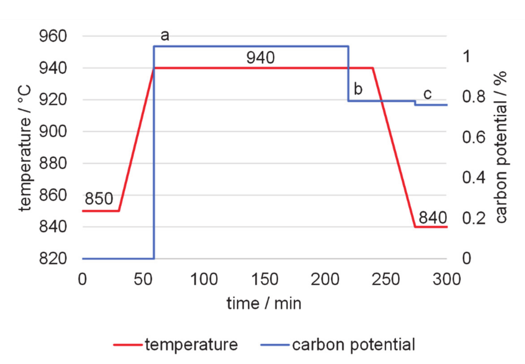
Figure 4.
Carbon profile (a), microhardness profile (b), and micrograph of cross section (c) of a sample with target case hardening depth of 0.5 mm.
Figure 4.
Carbon profile (a), microhardness profile (b), and micrograph of cross section (c) of a sample with target case hardening depth of 0.5 mm.

Figure 5.
Carbon profile (a), microhardness profile (b), and micrograph of cross section (c) of a sample with target case hardening depth of 1 mm.
Figure 5.
Carbon profile (a), microhardness profile (b), and micrograph of cross section (c) of a sample with target case hardening depth of 1 mm.
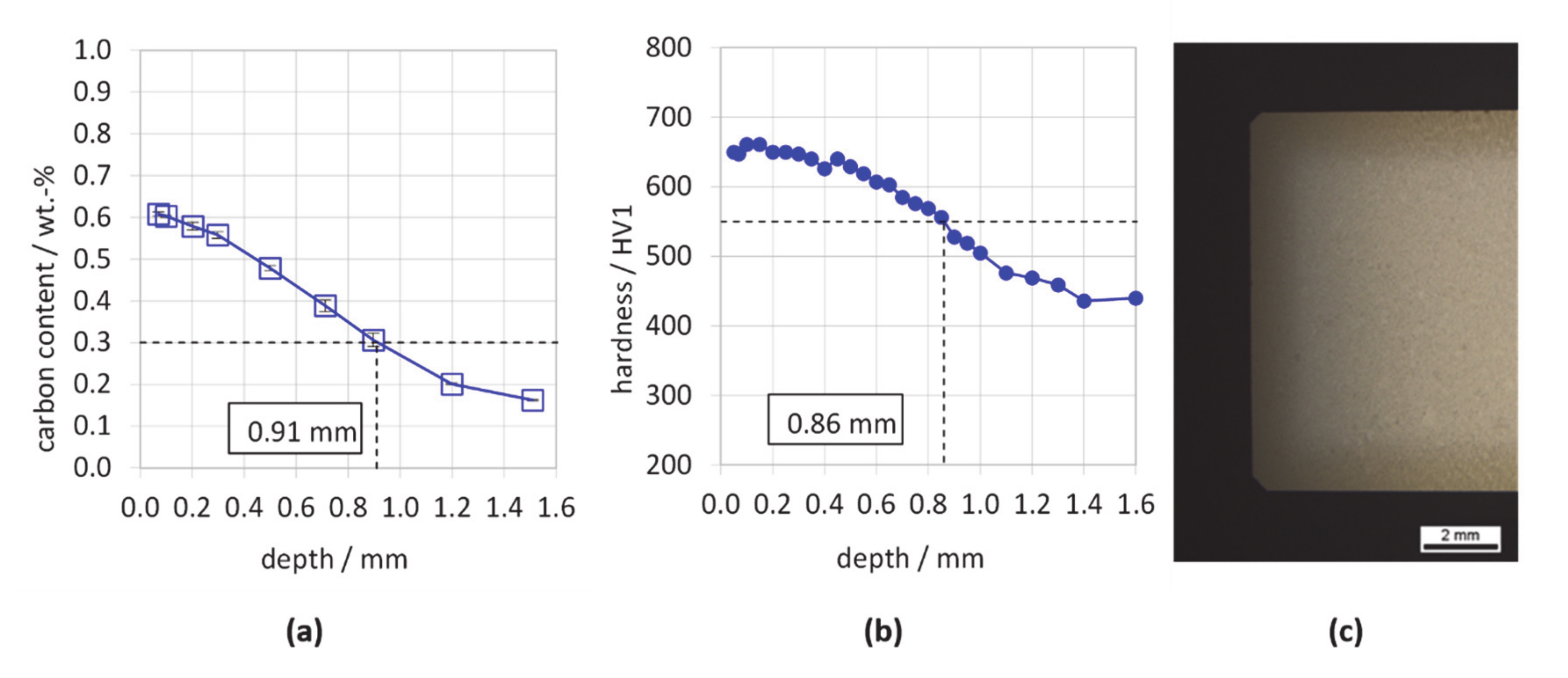
Figure 6.
Carbon profile (a), microhardness profile (b), and micrograph of cross section (c) of a sample with target case hardening depth of 2 mm.
Figure 6.
Carbon profile (a), microhardness profile (b), and micrograph of cross section (c) of a sample with target case hardening depth of 2 mm.

Figure 7.
Correlation of micromagnetic determined and actual measured hardness of the calibration data set without limitation of the maximum error effect (a) and with limitation to 3 HV1 (b).
Figure 7.
Correlation of micromagnetic determined and actual measured hardness of the calibration data set without limitation of the maximum error effect (a) and with limitation to 3 HV1 (b).

Figure 8.
Correlation of micromagnetic determined and actual measured hardness of the test data set without limitation of the maximum error effect (a) and with limitation to 3 HV1 (b).
Figure 8.
Correlation of micromagnetic determined and actual measured hardness of the test data set without limitation of the maximum error effect (a) and with limitation to 3 HV1 (b).
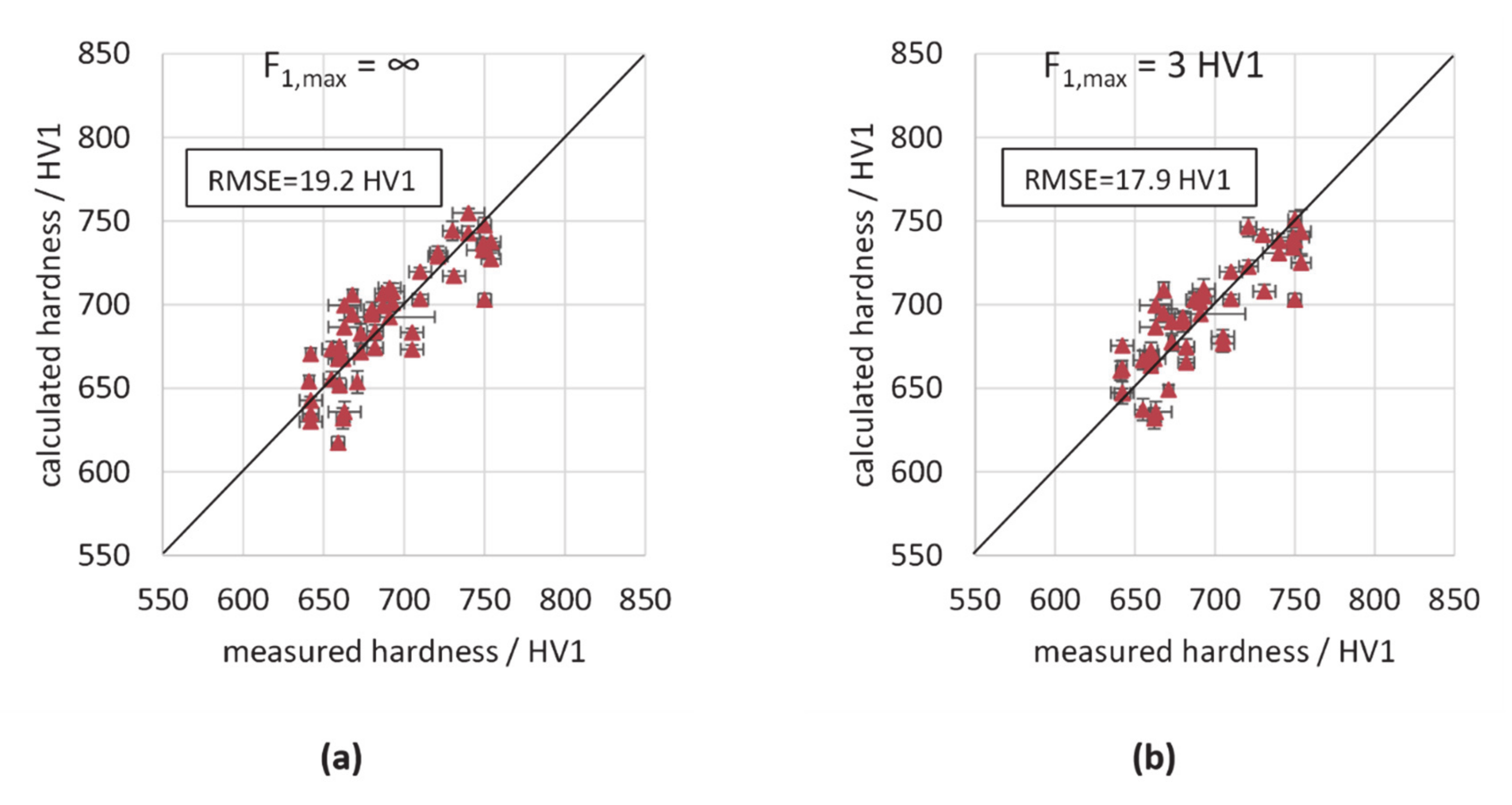
Figure 9.
Correlation between hardness and amplitude at the remanence point of the incremental permeability µr measured with a base magnetization frequency of 120 Hz and an eddy current loop frequency of 100 kHz (a) and a base magnetization frequency of 150 Hz and an eddy current loop frequency of 250 kHz (b).

Figure 10.
Correlation of micromagnetic determined and actual measured carburization depth of the calibration data set without limitation of the maximum error effect (a) and with limitation to 0.06 mm (b).
Figure 10.
Correlation of micromagnetic determined and actual measured carburization depth of the calibration data set without limitation of the maximum error effect (a) and with limitation to 0.06 mm (b).
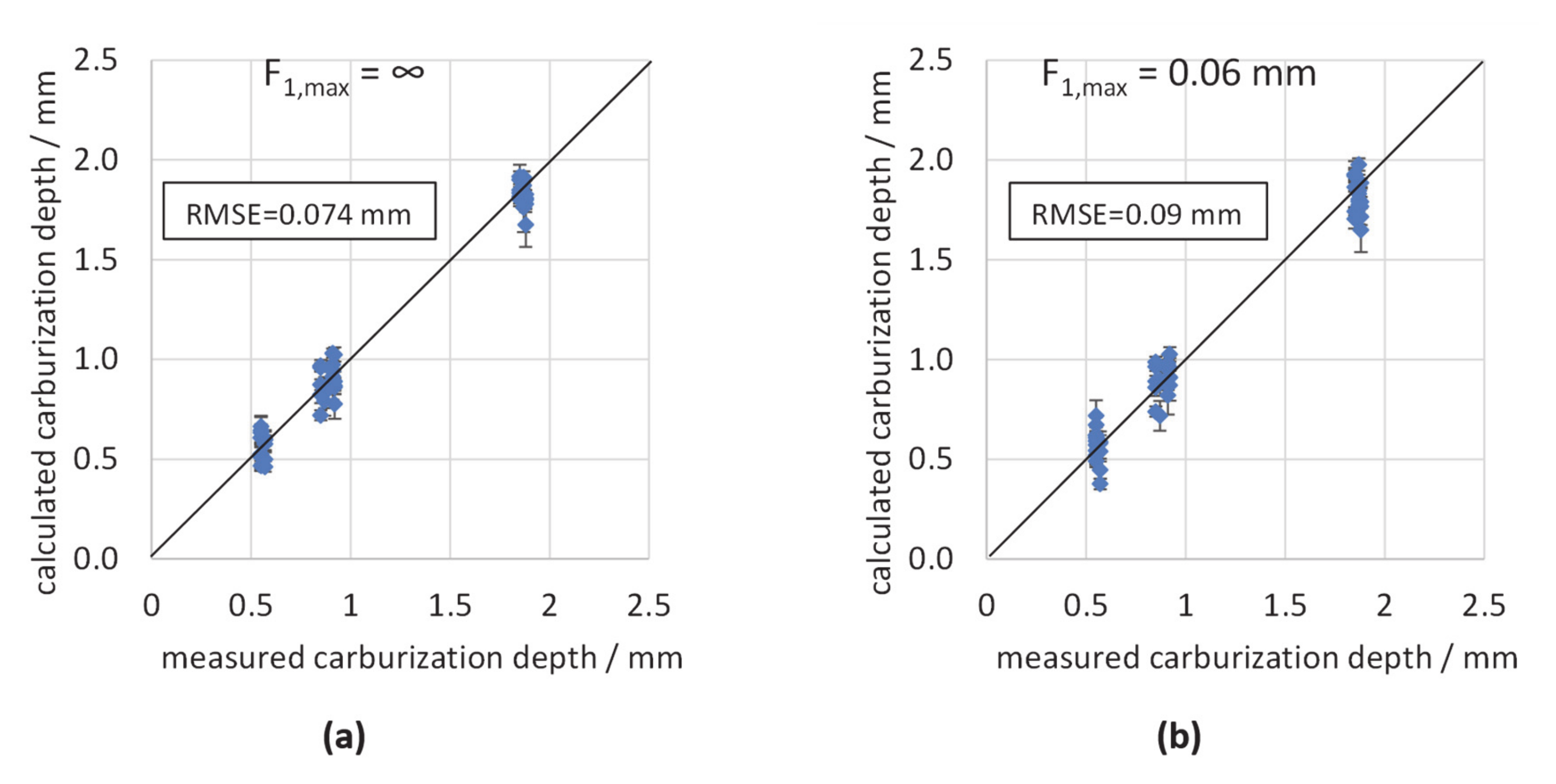
Figure 11.
Correlation of micromagnetic determined and actual measured carburization depth of the test data set without limitation of the maximum error effect (a) and with limitation to 0.06 mm (b).
Figure 11.
Correlation of micromagnetic determined and actual measured carburization depth of the test data set without limitation of the maximum error effect (a) and with limitation to 0.06 mm (b).

Figure 12.
Correlation of micromagnetic determined and actual measured hardness of the training data set after 30 (a) and 60 (b) repetitions of the training lesson using artificial neural networks (ANNs).
Figure 12.
Correlation of micromagnetic determined and actual measured hardness of the training data set after 30 (a) and 60 (b) repetitions of the training lesson using artificial neural networks (ANNs).
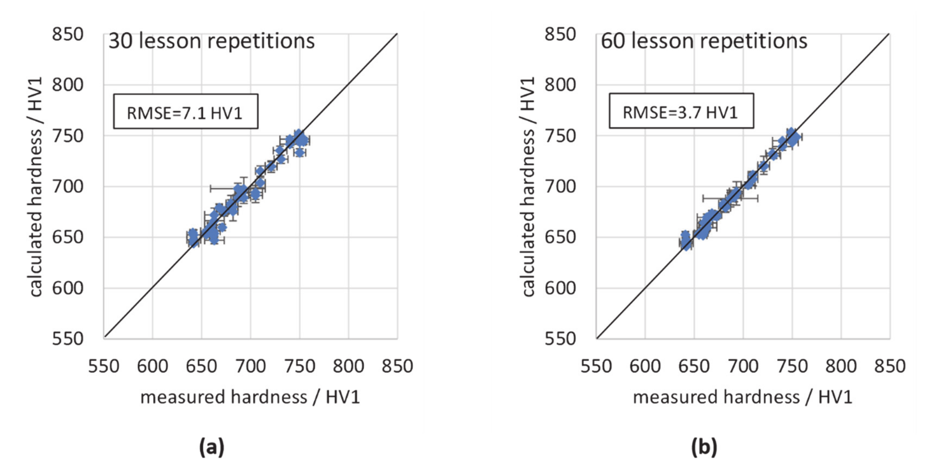
Figure 13.
Correlation of micromagnetic determined and actual measured hardness of the test data set after 30 (a) and 60 (b) repetitions of the training lesson using ANN.
Figure 13.
Correlation of micromagnetic determined and actual measured hardness of the test data set after 30 (a) and 60 (b) repetitions of the training lesson using ANN.

Figure 14.
Correlation of micromagnetic determined and actual measured carburization depth after 30 repetitions of the training lesson for training (a) and test data set (b).
Figure 14.
Correlation of micromagnetic determined and actual measured carburization depth after 30 repetitions of the training lesson for training (a) and test data set (b).

Figure 15.
Correlation of micromagnetic determined (linear regression) and actual measured hardness of calibration and test data set with standard configuration (a) and use of sweeps (b).
Figure 15.
Correlation of micromagnetic determined (linear regression) and actual measured hardness of calibration and test data set with standard configuration (a) and use of sweeps (b).
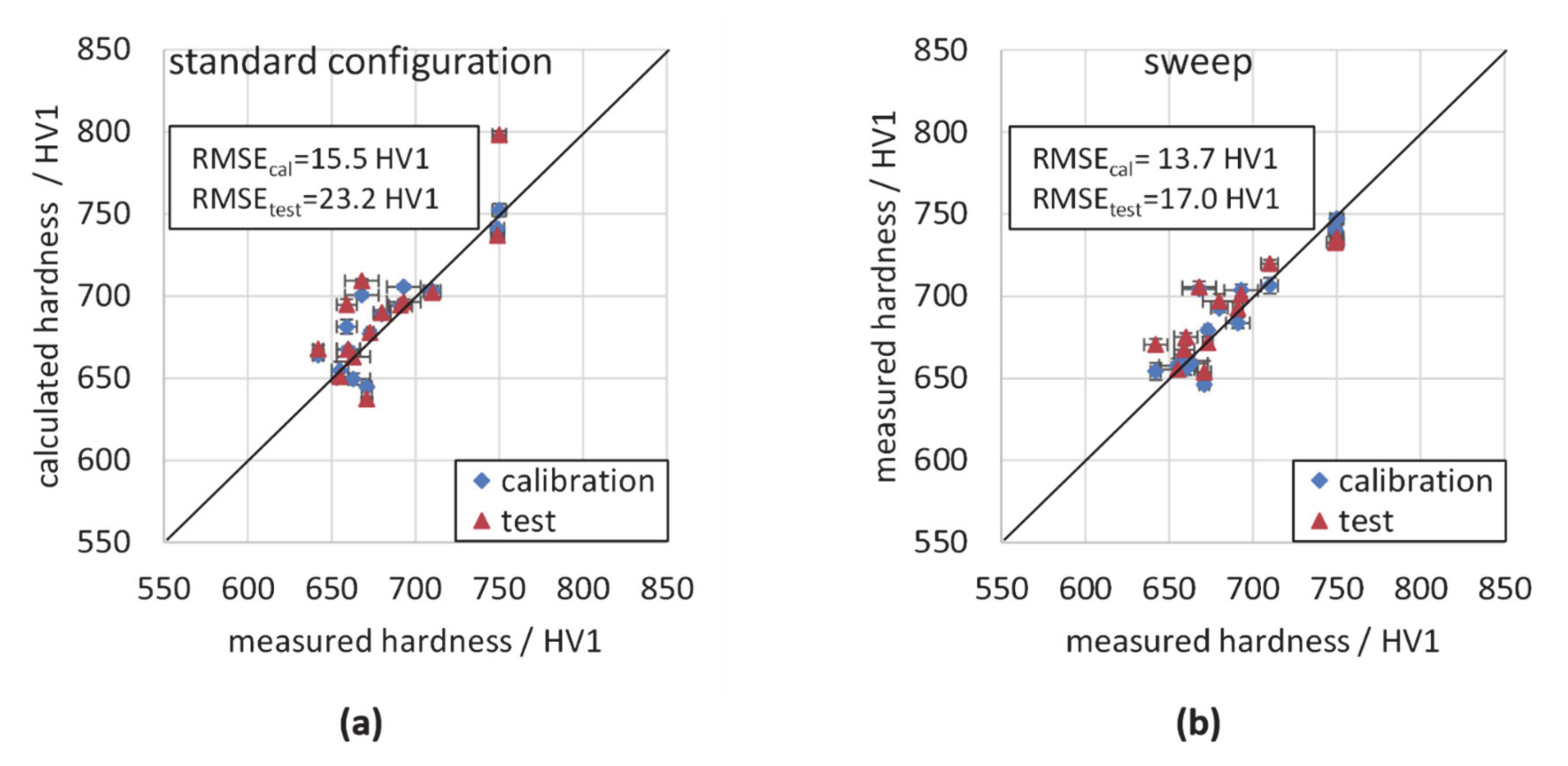
Table 1.
Measured chemical composition of the AISI 4820 in wt. %.
| C | Si | Mn | P | S | Cr | Mo | Ni |
|---|---|---|---|---|---|---|---|
| 0.17 | 0.39 | 0.51 | 0.01 | <0.002 | 1.56 | 0.26 | 1.43 |
Table 2.
Heat treatment variations (target values).
| Surface Carbon Content/wt. % | Case Hardening Depth/mm | Tempering Temperature/°C |
|---|---|---|
| 0.6/0.7/0.8 | 0.5/1/2 | 150/180/210 |
Table 3.
Holding times at the different temperatures and carbon potential in the atmosphere for the different heat treatment variations.
Table 3.
Holding times at the different temperatures and carbon potential in the atmosphere for the different heat treatment variations.
| Variation | 850 °C | a | 940 °C | b | 840 °C | c |
|---|---|---|---|---|---|---|
| 0.5 mm, 0.6 wt. % | 30 min | 0.9 vol. % | 20 min | 0.57 vol. % | 30 min | 0.57 vol. % |
| 0.5 mm, 0.7 wt. % | 30 min | 0.9 vol. % | 80 min | 0.68 vol. % | 30 min | 0.68 vol. % |
| 0.5 mm, 0.8 wt. % | 30 min | 0.9 vol. % | 80 min | 0.79 vol. % | 30 min | 0.79 vol. % |
| 1 mm, 0.6 wt. % | 30 min | 1.0 vol. % | 200 min | 0.55 vol. % | 30 min | 0.55 vol. % |
| 1 mm, 0.7 wt. % | 30 min | 1.05 vol. % | 180 min | 0.68 vol. % | 30 min | 0.66 vol. % |
| 1 mm, 0.8 wt. % | 30 min | 1.05 vol. % | 180 min | 0.78 vol. % | 30 min | 0.76 vol. % |
| 2 mm, 0.6 wt. % | 120 min | 1.05 vol. % | 740 min | 0.55 vol. % | 60 min | 0.55 vol. % |
| 2 mm, 0.7 wt. % | 120 min | 1.1 vol. % | 720 min | 0.65 vol. % | 60 min | 0.64 vol. % |
| 2 mm, 0.8 wt. % | 120 min | 1.1 vol. % | 720 min | 0.75 vol. % | 60 min | 0.75 vol. % |
Table 4.
Configuration of the 3MA-measurements.
| Standard Configuration | ||
| Method | Magnetization Frequency | 120 Hz |
| Harmonic analysis (HA) | Magnetization amplitude | 75 A/cm |
| Barkhausen noise (BN) | Magnetization amplitude | 75 A/cm |
| Highpass frequency | 100 kHz | |
| Lowpass frequency | No limitation | |
| Incremental permeability (IP) | Magnetization amplitude | 75 A/cm |
| Eddy current frequency | 250 kHz | |
| Eddy current (EC) | Magnetization amplitude | 65 A/cm |
| Frequencies | 3,5 kHz, 1 MHz, 2 MHz, 5 MHz | |
| Sweeps | ||
| HA, BN, IP | Magnetization frequency | 20 Hz, 30 Hz, 40 Hz, 50 Hz, 60 Hz, 80 Hz, 100 Hz, 150 Hz, 200 Hz, 250 Hz, 300 Hz, 350 Hz |
| BN | High pass frequency | no limitation, 500 kHz, 1 MHz |
| IP | Eddy current frequency | 10 kHz, 20 kHz, 60 kHz, 80 kHz, 100 kHz, 150 kHz, 200 kHz, 300 kHz, 350 kHz |
Table 5.
Coefficient of determination and standard error in dependence of the maximum error effect for regression analysis of hardness.
Table 5.
Coefficient of determination and standard error in dependence of the maximum error effect for regression analysis of hardness.
| F1,max/HV1 | F1/HV1 | R2 | RMSE/HV1 |
|---|---|---|---|
| ∞ | 9.274 | 0.8709 | 12.919 |
| 9 | 5.582 | 0.8772 | 12.599 |
| 5 | 4.887 | 0.8662 | 13.151 |
| 4 | 3.489 | 0.8669 | 13.116 |
| 3 | 2.819 | 0.8571 | 13.59 |
| 2 | 1.899 | 0.837 | 14.514 |
| 1 | 0.961 | 0.723 | 18.923 |
Table 6.
Overview of the regression results for hardness (calibration data set).
| F1,max = ∞ | F1,max = 3 HV1 | ||
|---|---|---|---|
| 2882.68 | 1 | 1640.43 | 1 |
| −44.3 | A3 (120 Hz) | −697.51 | A7 (100 Hz) |
| −3397.44 | Mmax (350 Hz) | −19.5 | P52 (30 Hz) |
| 274.2 | √P3 (50 Hz) | −0.36 | Hcm2 (80 Hz, HP 100 kHz) |
| −0.12 | Hco2 (50 Hz) | 411.53 | √A7 (100 Hz) |
| −142.44 | √DH25µ (120Hz, 60 kHz) | −5.59 | P72 (120 Hz) |
| −772.37 | √µr (120 Hz, 100 kHz) | −240.26 | √µr (120 Hz, 250 kHz) |
| 56.74 | P32 (150 Hz) | −1582.39 | √µr (150 Hz) |
| −33.69 | Vmag2 (350 Hz) | 1974.5 | Mr2 (350 Hz) |
| 7305.07 | Mmax2 (350 Hz) | −926.19 | √Mr (350 Hz) |
Table 7.
Maximum error effect, coefficient of determination, and standard error in dependence of the maximum number of regression terms for regression analysis of hardness.
Table 7.
Maximum error effect, coefficient of determination, and standard error in dependence of the maximum number of regression terms for regression analysis of hardness.
| Maximum Number of Regression Terms | F1/HV1 | R2 | RMSE/HV1 | RMSEtest/HV1 |
|---|---|---|---|---|
| 20 | 581.163 | 0.9457 | 8.375 | 13.5 |
| 10 | 9.274 | 0.8709 | 12.919 | 19.2 |
| 8 | 6.738 | 0.8548 | 13.7 | - |
| 6 | 7.174 | 0.8198 | 15.260 | 18.7 |
| 4 | 3.916 | 0.7674 | 17.341 | - |
| 2 | 3.496 | 0.6183 | 22.210 | - |
Table 8.
Coefficient of determination and standard error in dependence of the maximum error effect for regression analysis of carburization depth.
Table 8.
Coefficient of determination and standard error in dependence of the maximum error effect for regression analysis of carburization depth.
| F1,max/mm | F1/mm | R2 | RMSE/mm |
|---|---|---|---|
| ∞ | 0.267 | 0.9539 | 0.117 |
| 0.2 | 0.191 | 0.9495 | 0.123 |
| 0.1 | 0.084 | 0.949 | 0.124 |
| 0.08 | 0.076 | 0.927 | 0.148 |
| 0.07 | 0.069 | 0.9246 | 0.150 |
| 0.06 | 0.059 | 0.9446 | 0.129 |
| 0.05 | 0.038 | 0.9333 | 0.141 |
| 0.03 | 0.029 | 0.9423 | 0.131 |
Table 9.
Overview of the regression results for carburization depth (calibration data set).
| F1,Max = ∞ | F1,Max = 0.06 mm | ||
|---|---|---|---|
| −25.23 | 1 | 14.39 | 1 |
| 46.78 | √Vmag (30 Hz) | 0.72 | K (300 Hz) |
| −1.82 | √P3 (30 Hz) | −6.16 | √P3 (40 Hz) |
| 9.25 | √µmax (30 Hz) | −0.08 | P72 (50 Hz) |
| −0.07 | P72 (50 Hz) | 0.7 | √Hco (50 Hz) |
| 0.001 | Hcm2 (80 Hz) | −0.0005 | DH50m 2 (80 Hz) |
| −4.7 | Vmag2 (150 Hz) | −7.87 | √Ph3 (120 Hz) |
| 0.66 | √K (200 Hz) | 0.005 | Hcm2 (250 Hz) |
| 0.44 | √P3 (250 Hz) | −0.0003 | DH25µ2 (250 Hz) |
| 0.36 | √Hco (350 Hz) | −0.31 | Vmag2 (350 Hz) |
Table 10.
Maximum error effect, coefficient of determination, and standard error in dependence of the maximum number of regression terms for regression analysis of carburization depth.
Table 10.
Maximum error effect, coefficient of determination, and standard error in dependence of the maximum number of regression terms for regression analysis of carburization depth.
| Maximum Number of Regression Terms | F1/mm | R2 | RMSE/mm | RMSEtest/mm |
|---|---|---|---|---|
| 20 | 180.252 | 0.984 | 0.069 | 0.315 |
| 10 | 0.267 | 0.9539 | 0.117 | 0.130 |
| 8 | 0.178 | 0.9421 | 0.132 | - |
| 6 | 0.115 | 0.9198 | 0.155 | 0.156 |
| 4 | 0.06 | 0.842 | 0.217 | - |
| 2 | 0.047 | 0.5361 | 0.372 | - |
Table 11.
Standard error based on a test data set of 14 samples for calibration with standard configuration and use of sweeps.
Table 11.
Standard error based on a test data set of 14 samples for calibration with standard configuration and use of sweeps.
| Calibration Method | Hardness | Carburization Depth | ||
|---|---|---|---|---|
| - | RMSEcal/HV1 | RMSEtest/HV1 | RMSEcal/mm | RMSEtest/mm |
| linear regression (standard configuration) | 15.5 | 23.2 | 0.12 | 0.22 |
| linear regression (sweep) | 13.7 | 17.0 | 0.07 | 0.13 |
| ANN (standard configuration) | 12.7 | 15.0 | 0.06 | 0.13 |
| ANN (sweep) | 7.2 | 16.5 | 0.02 | 0.04 |
Table 12.
Overview of the standard error for the different types of calibration.
| Calibration Method | Hardness | Carburization Depth | ||
|---|---|---|---|---|
| - | RMSEcal/HV1 | RMSEtest/HV1 | RMSEcal/mm | RMSEtest/mm |
| linear regression (F1,max unlim.) | 12.1 | 19.1 | 0.074 | 0.130 |
| linear regression (F1,max lim.) | 12.5 | 17.9 | 0.090 | 0.140 |
| ANN (30 repetitions) | 7.1 | 16.4 | 0.030 | 0.103 |
| ANN (60 repetitions) | 3.7 | 18.6 | - | - |
Publisher’s Note: MDPI stays neutral with regard to jurisdictional claims in published maps and institutional affiliations. |
© 2020 by the authors. Licensee MDPI, Basel, Switzerland. This article is an open access article distributed under the terms and conditions of the Creative Commons Attribution (CC BY) license (http://creativecommons.org/licenses/by/4.0/).
Share and Cite
MDPI and ACS Style
Jedamski, R.; Epp, J. Non-Destructive Micromagnetic Determination of Hardness and Case Hardening Depth Using Linear Regression Analysis and Artificial Neural Networks. Metals 2021, 11, 18. https://doi.org/10.3390/met11010018
AMA Style
Jedamski R, Epp J. Non-Destructive Micromagnetic Determination of Hardness and Case Hardening Depth Using Linear Regression Analysis and Artificial Neural Networks. Metals. 2021; 11(1):18. https://doi.org/10.3390/met11010018
Chicago/Turabian StyleJedamski, Rahel, and Jérémy Epp. 2021. "Non-Destructive Micromagnetic Determination of Hardness and Case Hardening Depth Using Linear Regression Analysis and Artificial Neural Networks" Metals 11, no. 1: 18. https://doi.org/10.3390/met11010018
Note that from the first issue of 2016, this journal uses article numbers instead of page numbers. See further details here.