Forming Mechanism of Weld Cross Section and Validating Thermal Analysis Results Based on the Maximal Temperature Field for Laser Welding

Abstract

In this paper, the forming mechanism of weld cross sections (WCSs) was studied via thermal analysis. The melting of a WCS was first dominated by heat convection from the flowing melt until the WCS had the max cross section in the transient temperature field. Then, the melting was dominated by heat conduction from the residual heat in the weld pool, giving rise to an increase in middle width but a decrease in upper and bottom width. This indicated that the WCS obtained from the transient temperature field could not represent the section after solidification. Therefore, thermal analysis results should be validated using the WCS obtained from the maximal temperature field. This WCS was dependent upon the max temperature of each node over time. Compared with the former WCS, the latter one showed better adaptability in terms of multi-process parameters when the thermal analysis results were validated.

1. Introduction

The thermal–metallurgical–mechanical coupling simulation is an important method to predict the behaviors caused by nonlinear thermal effects in laser-welded structures [1,2]. The predicted behaviors involve phase distribution [3], hardness [4,5], distortions [6,7] and residual stresses [8,9]. The peak temperature and heating/cooling rate vary rapidly at different positions and times during welding, leading to highly inconsistent behavior in the metallurgical and mechanical elements of weld joints. The simulation is commonly performed through a sequentially-coupled model and finite element modeling [10], and thus the predicted accuracy is strongly associated with the thermal analysis. In a welding thermal analysis, the main difficulties are the modeling and validating of heat source models.

As heat source models reflect realistic welding energy distributions, the accuracy of thermal analysis is highly dependent upon if they are reasonable or not. The models mainly include four types: point [11], surface [12], volume [13] and a combination of the former three [14]. In the four type models, the combined heat source model shows better accuracy and flexibility. The model is commonly combined in terms of volume–volume and volume–surface. Wang et al. [15] carried out polynomial fitting to the representative WCS of partial and fully penetrated welds and established associated combined models based on the fitted functions. The predicted results showed good agreement with the experimental section, with an error of 8.7% in terms of area. As the WCS of fully penetrated weld had a waist contraction characteristic, Rong et al. [1] and Zhan et al. [16] established bi-pyramidal heat source models to improve the accuracy. All of the above models were modelled according to the shape characteristics of associated WCSs. In fact, keyholes act as heat sources, transferring heat to melt the surrounding metal during keyhole laser welding, and this results in the formation of weld pools and WCSs. Xu et al. [17] established a double cylindrical heat source model considering the keyhole angle and diameter, and the model had good adaptability in terms of multi-process parameters.

In the other hand, validating heat source models is an important step for welding thermal analysis. Researchers tend to use WCSs [16,18,19], thermal cycles [20,21] or a combination of both [22,23,24] obtained from experiments to validate the models. It is worth noting that, in most studies, the section used for validating is a section obtained from the transient temperature field. The section is commonly selected depending on the experience of the researchers and can take the form of, for example, the section at the position which has the max upper width in the weld pool. However, the residual heat in the weld pool would continue melt the metal of the section, and therefore the section from the weld pool cannot not represent the section after solidification. Therefore, validating using the section could mislead researchers and result in larger errors in sequentially-coupled thermal–metallurgical–mechanical finite element analysis.

Therefore, in this paper, as a development of our previous studies [17], we studied the forming mechanism of WCSs and validated the thermal analysis results based on the maximal temperature field for laser welding. The rules relating to changes in the upper/bottom/waist widths over time were calculated from the transient temperature field. The forming mechanism of the WCS was analyzed according to the results. The WCS obtained from the transient temperature field was compared with that obtained from the maximal temperature field with the aim of clarifying their effects on the accuracy of thermal analysis.

2. Experiment Details and Numerical Modeling

2.1. Experiment Details

In our previous studies [17], laser butt welding experiments using six different welding speeds (2.4, 3.3, 4.2, 5.1, 6.0, 6.9 m/min) were performed, and the laser power was 4 kW. The base material was ultra-high strength steel 1700MS from SSAB of Sweden, and the sheet dimension was 100 mm × 50 mm × 2 mm. The laser power was 4 kW, and the defocusing distance was 0 mm.

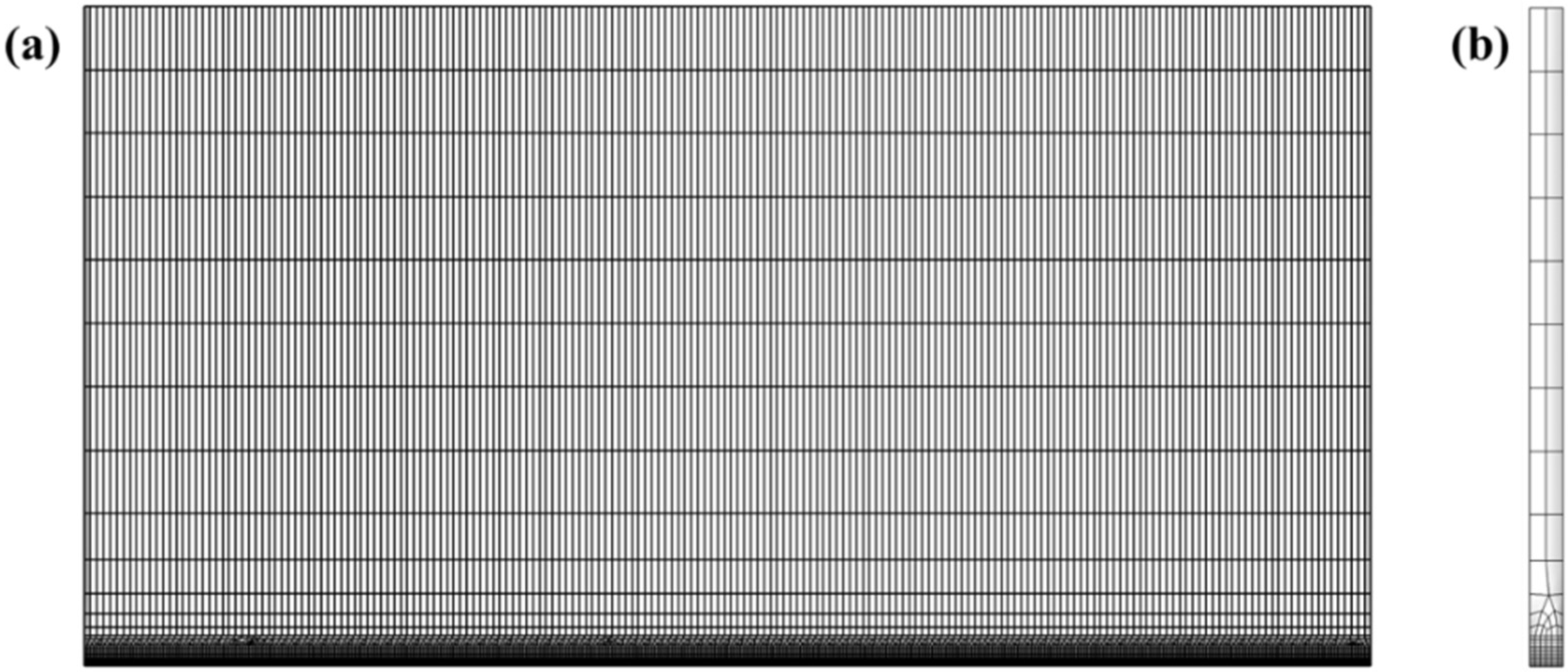
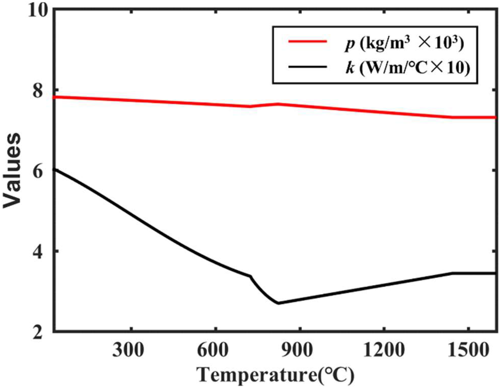
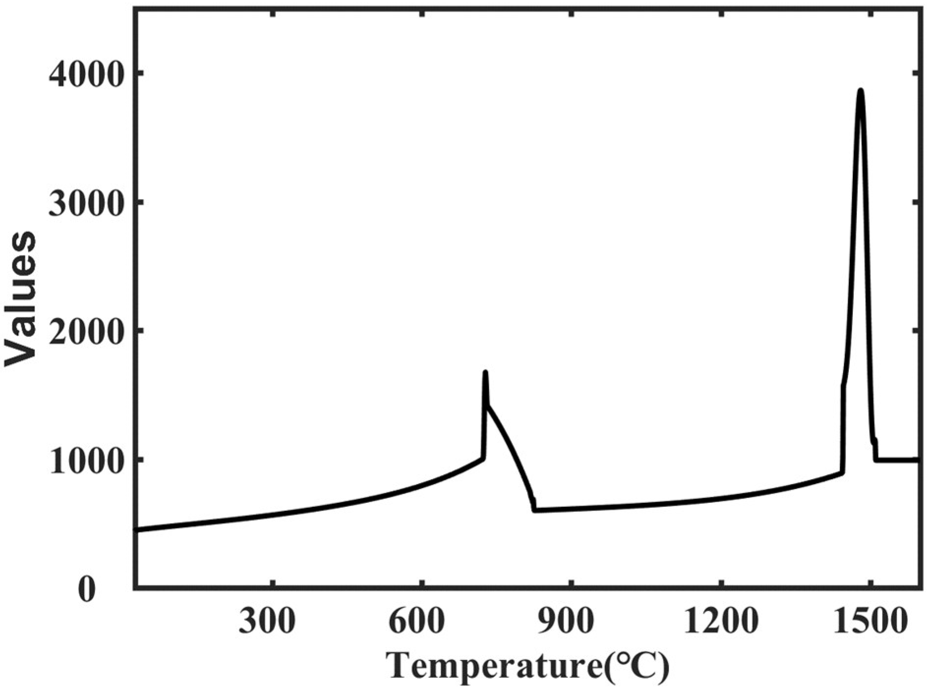
2.2. Governing Equations and Boundary Conditions

In this paper, the transient heat conduction equation was expressed as follows:

$$\rho (T)C(T)\frac{\partial T}{\partial t}=\frac{\partial }{\partial x}\left[k(T)\frac{\partial T}{\partial x}\right]+\frac{\partial }{\partial y}\left[k(T)\frac{\partial T}{\partial y}\right]+\frac{\partial }{\partial z}\left[k(T)\frac{\partial T}{\partial z}\right]+q(x,y,z)$$

(1)

where ρ(T), k(T) and C(T) were the temperature-dependent density, thermal conductivity and specific heat capacity, respectively, and q(x, y, z) was the heat flux distribution of the laser.

The transient thermal fields were solved using the commercial ANSYS APDL code. The finite element model of the weld sheets is presented in Figure 1. The mesh in and near the weld zone was refined, and the minimum mesh was 0.2 mm × 0.12 mm × 0.25 mm in size. Due to the symmetry load and geometry, only half of the finite element model was modelled. The numbers of element and nodes were 45,322 and 56,970.

During the welding process, radiation losses dominated for higher temperatures near the weld zone and convection losses for lower temperatures away from the weld zone. Therefore, heat losses during welding were simplified to be an equivalent heat transfer coefficient h_c shown as Equation (2) [25], and the coefficient was applied to all of the free surfaces, except the symmetry plane, for thermal boundary conditions. The temperature-dependent material properties of 1700MS are shown in Figure 2 and Figure 3.

$$h_c\left(T\right)=\{\begin{array}{cc}0.0668T& T\le 500°\mathrm{C}\\ 0.231T-82.1& T>500°\mathrm{C}\end{array}$$

(2)

2.3. Heat Source Model

During keyhole laser welding, most of the laser energy is absorbed by the keyhole. The keyhole acts as a heat source which transfers heat to melt the surrounding metal, and this results in the formations of the weld pool and WCS after solidification [26]. Meanwhile, fully penetrated WCSs have a “bi-pyramidal” shape with narrow middle and wide upper/bottom ends. This indicates that the energy in the keyhole was mainly concentrated in the upper/bottom areas. Therefore, this paper used a double cylindrical heat source model accordingly to the diameter and incline angle of the keyhole [17]. The model considered the following assumptions:

• The keyhole had the shape of a cylinder with a fixed diameter in the thickness direction.
• The peak of the heat flux decayed exponentially with an increase in the distance to the upper or bottom surfaces.
• Convective heat transfer in weld pool was not considered.

Compared with previous heat sources, which were usually modelled based on WCSs, this model could simulate the welding process more realistically. The mathematical expression of the model is shown in Equations (3)–(5), where h₁ and Q_L1 are the height and laser power of the upper heat source, h₂ and Q_L2 are the height and laser power of the bottom heat source, a is the heat source angle (keyhole incline angle), f₁ is the radius coefficients, f₂ is the decay index of the heat flux in the thickness direction, H is the total heat source height, and λ is the welding efficiency. Further information can be found in reference [17].

$$q(x,y,z)=q_1(x,y,z)+q_2(x,y,z)$$

(3)

$$\begin{array}{c}{q}_1(x,y,z)=\frac{9\lambda Q_{L1}}{\pi f_1^2{h}_1{r}_0{}^2{\left(1-e^{-3}\right)}^2}\exp \left[3\frac{x\sin (\alpha )+z\cos (\alpha )-f_1{r}_0\sin (\alpha )}{h_1}\right]\\ \times \exp \left(-f_2\frac{{\left[x\cos (\alpha )-z\sin (\alpha )+f_1{r}_0-f_1{r}_0\cos (\alpha )\right]}^2+y^2}{{\left(f_1{r}_0\right)}^2}\right)\end{array}$$

(4)

$$\begin{array}{c}{q}_2(x,y,z)=\frac{9\lambda Q_{L2}}{\pi f_1^2{h}_2{r}_0{}^2{\left(1-e^{-3}\right)}^2}\exp \left[-3\frac{H+x\sin \left(\alpha \right)+z\cos \left(\alpha \right)-f_1{r}_0\sin \left(\alpha \right)}{h_2}\right]\\ \times \exp \left(-f_2\frac{{\left[x\cos (\alpha )-z\sin (\alpha )+f_1{r}_0-f_1{r}_0\cos (\alpha )\right]}^2+y^2}{{\left(f_1{r}_0\right)}^2}\right)\end{array}$$

(5)

3. Results and Discussion

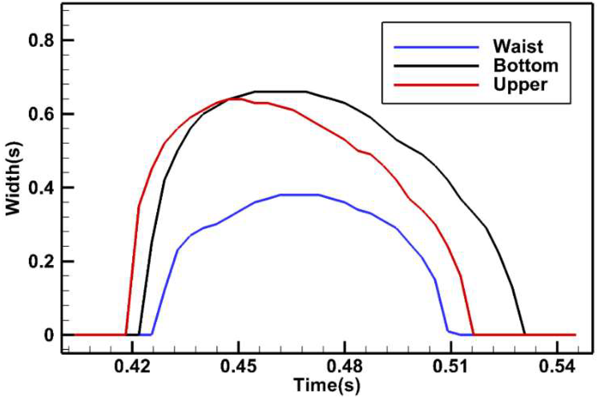
3.1. Rule of Upper/Bottom/Waist Width Changes over Time

In a welding thermal analysis, the predicted weld pool has the same shape except for at the beginning and end of the solution, so the weld pool during the middle part can be used to represent the predicted results. A 3D weld pool at 0.447 s using a weld speed of 3.3 m/min is shown in Figure 4. The predicted upper/bottom widths and upper length were 1.28 mm, 1.34 mm and 5.36 mm, respectively, with errors of 8.47%, 9.84% and 9.86%, respectively, compared to the experiment results in

Table 1. Predicted upper/bottom/waist widths of the two WCSs using different welding speeds.

Welding Speed (m/min)		2.4	3.3	4.2	5.1	6.0	6.9
Upper width (mm)	Experiment	1.34	1.13	1.01	0.97	0.96	0.83
	Simulation (Transient)	1.42	1.28	1.16	1.06	0.98	0.92
	Simulation (Max)	1.42	1.28	1.16	1.06	0.98	0.92
Bottom width (mm)	Experiment	1.43	1.19	1.04	0.95	0.85	0.69
	Simulation (Transient)	1.50	1.28	1.10	1.00	0.94	0.78
	Simulation (Max)	1.54	1.34	1.16	1.02	0.94	0.80
Waist width (mm)	Experiment	0.78	0.66	0.58	0.54	0.48	0.42
	Simulation (Transient)	0.82	0.64	0.56	0.52	0.42	0.28
	Simulation (Max)	0.92	0.74	0.60	0.58	0.52	0.48
Relative root mean square error (%)	Simulation (Transient)	5.35	8.99	10.21	6.52	9.53	21.59
	Simulation (Max)	12.48	10.12	10.81	7.44	7.20	11.87

. The longitudinal section at the symmetry plane (x = 24 mm) had an asymmetrical shape with narrow middle and wide upper/bottom ends (Figure 4b). Both of the front and rear walls in the weld pool concaved towards the middle, and the rear wall had a larger concavity than the front wall. The shape had a good level of consistency with the fully penetrated longitudinal sections of the experimental research performed by Zhang et al. [27], indicating the heat source model could satisfactorily predict the 3D shapes of weld pools.

In terms of validation, the difference between the predicted and experimental WCSs is commonly used to evaluate the predicted accuracy. It is essential to validate the thermal analysis result using the WCS obtained from the maximal temperature field. This is due to the fact that the WCS from the transient temperature field cannot possess max upper/bottom/waist widths simultaneously, and this can result in extra errors. Taking the WCS at 0.447 s as an example, the section is shown on the plane x = 24 mm in Figure 4d, and changes in its upper/bottom/waist widths over time are shown in Figure 5. It can be seen that the times when the widths reached their maximum were 0.447 s, 0.455 s and 0.462 s. The corresponding max widths were 1.28 mm, 1.36 mm and 0.74 mm, while the widths in Figure 4d were 1.28 mm, 1.28 mm and 0.62 mm. The bottom and waist widths had differences of 0.08 mm and 0.12 mm. Validation using the WCS in Figure 4d could result in extra errors of 5.88% (bottom width) and 16.2% (waist width).

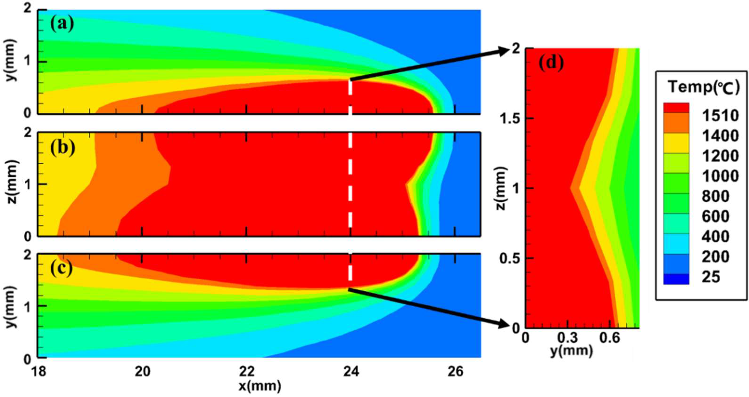
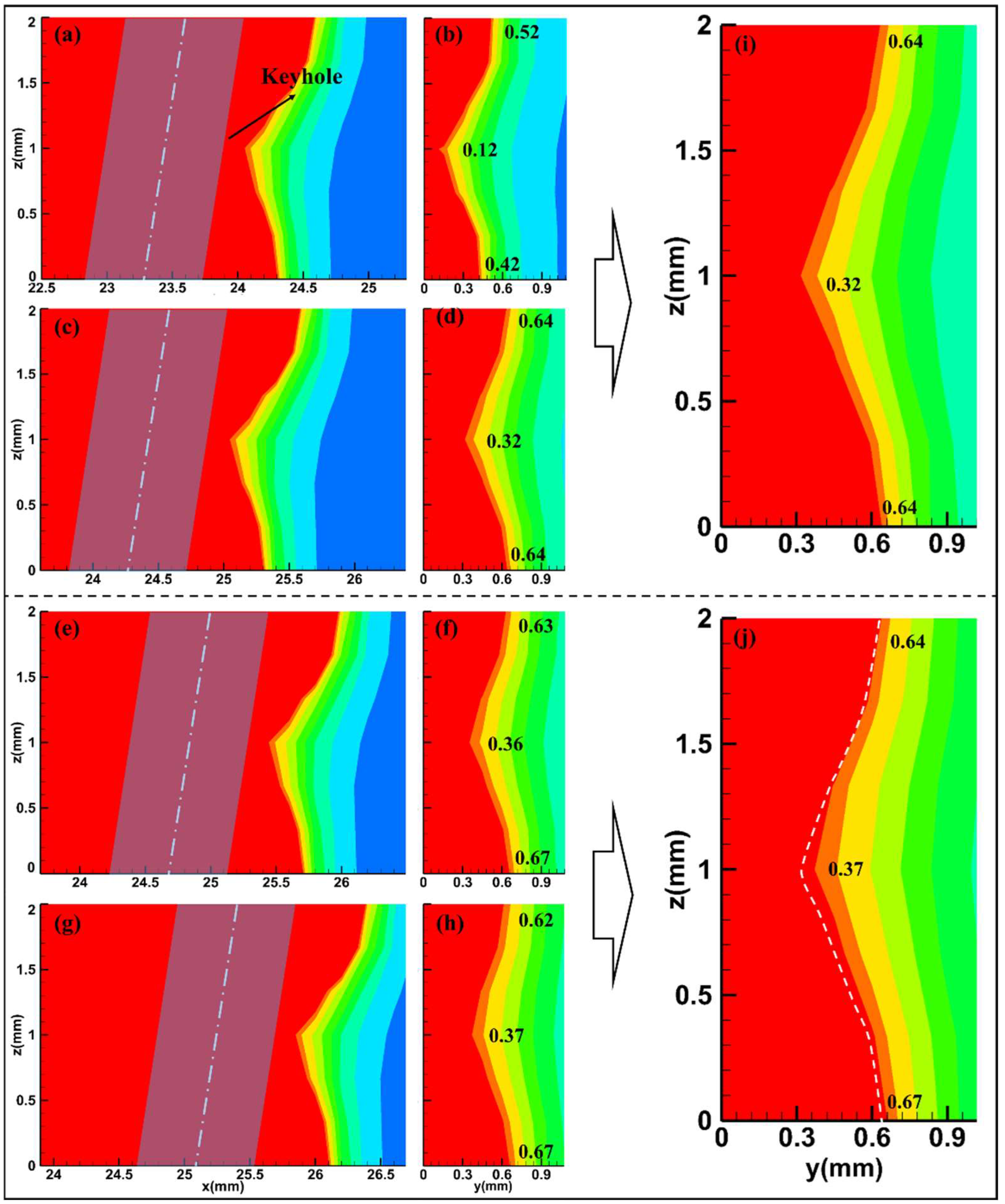
3.2. Formation Mechanism of WCS

Figure 6 shows the forming process of the WCS at x = 24 mm. The longitudinal sections and cross sections obtained from the transient temperature field are shown in Figure 6a–h. The WCSs obtained from the maximal temperature field at 0.447 s and 0.462 s are shown in Figure 6i,j, respectively, namely the max temperature of each node over time until 0.447 s and 0.462 s. The forming process can be divided into two phases. Phase Ⅰ was from 0.429 s to 0.447 s, when heat transfer was dominated by convection. Phase Ⅱ was from 0.447 s to 0.462 s, when heat transfer was dominated by conduction.

During Phase Ⅰ, the keyhole began to move through the plane x = 24 mm at 0.429 s, as shown as Figure 6a. The metal near the keyhole was vaporized by the high-power density laser, and, meanwhile, the melt flowed rapidly due to the action of vapor recoil pressure. The flowing melt then transferred heat to melt more metal at the plane x = 24 mm. The upper/bottom/waist widths were 0.52/0.42/0.12 mm, respectively, as shown in Figure 6b. The WCS increased, with the keyhole moving, until 0.447 s (Figure 6c,d).

After the keyhole moved through the plane x = 24 mm, the flow velocities at the plane decreased and the heat was also transferred by convection. When the heat convection decreased to a certain degree, the metal at the plane was mainly melted by heat conduction from the residual heat in the weld pool, and thus heat transfer was dominated by conduction in Phase II. Compared with Phase I, the size of the WCS did not continuously increase during Phase II. The bottom/waist widths continued to increase with time, while the upper width decreased, as shown in Figure 6e–g. It is worth noting that the WCSs increased during both Phase I and Phase II, as shown in Figure 6i,j. This indicates that the WCS obtained from the maximal temperature field, which showed the max-temperature of each node over time, was the final one after solidification. Therefore, thermal analysis validation should use this WCS instead of that obtained from the transient temperature field.

3.3. Comparation of the Validation Results Based on the WCSs Obtained from the Transient and Maximal Temperature Fields

Table 1 shows the predicted upper/bottom/waist widths based on the two WCSs when using different welding speeds. The six welding speeds used the same heat source parameters, f₁ = 1.00 and f₂ = 4.00, which were obtained through a trial-and-error method. It could be seen that the predicted upper widths had the same sizes. The reason for this was that the WCS obtained from the transient temperature field was selected according to the upper width, namely the section with a max upper width in the weld pool. The differences in the bottom widths were small, with values from 0 mm to 0.06 mm. Compared to the experiment results, the differences in relative error were from 0% to 5.88%. The differences between the two types of validation sections were mainly reflected in waist widths. The relative errors of the former were 12.82%, 16.2%, 0%, 6.90%, 11.1% and 71.4% smaller than the latter.

To calculate the error of the whole cross section, the relative root mean square error of simulation and experiment results were used as evaluation index, as shown as Equation (6) (Where w_i is the experiment results, l_i is the predicted result and the subscripts 1, 2 and 3 represent the upper/bottom/waist widths of WCS).

$$\Delta =\sqrt{\frac{1}{3}{\displaystyle \sum _{i=1}^3{\left(\frac{l_i-w_i}{w_i}\right)}^2}}$$

(6)

The mean error based on the WCS obtained from the transient temperature field was 10.23%, and the standard deviation was 5.82%. The mean error based on the WCS obtained from the maximal temperature field was 9.98%, and the standard deviation was 2.22%. It could be seen that the latter had better adaptability in terms of multi-process parameters from the two standard deviations. In addition, the residual heat in the weld pool would continue melt the metal perpendicular to the welding direction, so the former could not represent the section after solidification. Validating using the former WCS could mislead researchers, and result in larger errors in subsequent sequentially-coupled thermal–metallurgical–mechanical analysis.

4. Conclusions

In this paper, the forming mechanism of WCSs was investigated, and the thermal analysis results were validated based on the maximal temperature field for laser welding. The following conclusions were drawn.

In the results of the transient temperature field, the upper/bottom/waist widths of the WCS could not reach their maximums simultaneously. The reason for this was that the waist width of the WCS would continue to increase due to the residual heat in the weld pool. This indicated that the WCS was not the final one after solidification, and thus any validation using it could result in extra errors. Therefore, thermal analysis results should be validated using a WCS obtained from the maximal temperature field.

The mean error based on the former WCS was 10.23%, and the standard deviation was 5.82%. The mean error based on the latter WCS was 9.98%, and the standard deviation was 2.22%. Compared with the former, the latter showed better adaptability in terms of multi-process parameters when the thermal analysis results were validated.

References

1. Rong, Y.; Mi, G.; Xu, J.; Huang, Y.; Wang, C. Laser penetration welding of ship steel EH36: A new heat source and application to predict residual stress considering martensite phase transformation. Mar. Struct. 2018, 61, 256–267. [Google Scholar] [CrossRef]
2. Chen, W.; Xu, L.; Zhao, L.; Han, Y.; Jing, H.; Zhang, Y.; Li, Y. Thermo-mechanical-metallurgical modeling and validation for ferritic steel weldments. J. Constr. Steel Res. 2020, 166, 105948. [Google Scholar] [CrossRef]
3. O’Meara, N.; Abdolvand, H.; Francis, J.A.; Smith, S.D.; Withers, P.J. Quantifying the metallurgical response of a nuclear steel to welding thermal cycles. Mater. Sci. Technol. 2016, 32, 1517–1532. [Google Scholar] [CrossRef]
4. Hamelin, C.J.; Muránsky, O.; Smith, M.C.; Holden, T.M.; Luzin, V.; Bendeich, P.J.; Edwards, L. Validation of a numerical model used to predict phase distribution and residual stress in ferritic steel weldments. Acta Mater. 2014, 75, 1–19. [Google Scholar] [CrossRef]
5. Vignier, S.; Biro, E.; Hervé, M. Predicting the hardness profile across resistance spot welds in martensitic steels. Weld. World 2014, 58, 297–305. [Google Scholar] [CrossRef]
6. Rong, Y.; Xu, J.; Huang, Y.; Zhang, G. Review on finite element analysis of welding deformation and residual stress. Sci. Technol. Weld. Join. 2017, 23, 198–208. [Google Scholar] [CrossRef]
7. Tchoumi, T.; Peyraut, F.; Bolot, R. Influence of the welding speed on the distortion of thin stainless steel plates-Numerical and experimental investigations in the framework of the food industry machines. J. Mater. Process. Technol. 2016, 229, 216–229. [Google Scholar] [CrossRef]
8. Li, S.; Ren, S.; Zhang, Y.; Deng, D.; Murakawa, H. Numerical investigation of formation mechanism of welding residual stress in P92 steel multi-pass joints. J. Mater. Process. Technol. 2017, 244, 240–252. [Google Scholar] [CrossRef]
9. Jiang, W.; Chen, W.; Woo, W.; Tu, S.T.; Zhang, X.C.; Em, V. Effects of low-temperature transformation and transformation-induced plasticity on weld residual stresses: Numerical study and neutron diffraction measurement. Mater. Des. 2018, 147, 65–79. [Google Scholar] [CrossRef]
10. Lindgren, L.-E. Numerical modelling of welding. Comput. Methods Appl. Mech. Eng. 2006, 195, 6710–6736. [Google Scholar] [CrossRef]
11. Rosenthal, D. Mathematical theory of heat distribution during welding and cutting. Weld. J. 1941, 20, 220–234. [Google Scholar]
12. Eagar, T.W.; Tsai, N.S. Temperature Fields Produced by Traveling Distributed Heat Sources. Weld. J. 1983, 62, 346–355. [Google Scholar]
13. Goldak, J.; Chakravarti, A.; Bibby, M. A New Finite Element Model for Welding Heat Sources. Metall. Trans. B. 1984, 15, 299–305. [Google Scholar] [CrossRef]
14. Chukkan, J.R.; Vasudevan, M.; Muthukumaran, S.; Kumar, R.R.; Chandrasekhar, N. Simulation of laser butt welding of AISI 316L stainless steel sheet using various heat sources and experimental validation. J. Mater. Process. Technol. 2015, 219, 48–59. [Google Scholar] [CrossRef]
15. Wang, J.; Han, J.; Domblesky, J.P.; Yang, Z.; Zhao, Y.; Zhang, Q. Development of a new combined heat source model for welding based on a polynomial curve fit of the experimental fusion line. Int. J. Adv. Manuf. Technol. 2016, 87, 1985–1997. [Google Scholar] [CrossRef]
16. Zhan, X.; Mi, G.; Zhang, Q.; Wei, Y.; Ou, W. The hourglass-like heat source model and its application for laser beam welding of 6 mm thickness 1060 steel. Int. J. Adv. Manuf. Technol. 2017, 88, 2537–2546. [Google Scholar] [CrossRef]
17. Rong, Y.; Wang, L.; Wu, R.; Xu, J. Visualization and simulation of 1700MS sheet laser welding based on three-dimensional geometries of weld pool and keyhole. Int. J. Therm. Sci. 2022, 171, 107257. [Google Scholar] [CrossRef]
18. Wu, C.S.; Hu, Q.X.; Gao, J.Q. An adaptive heat source model for finite-element analysis of keyhole plasma arc welding. Comput. Mater. Sci. 2009, 46, 167–172. [Google Scholar] [CrossRef]
19. Derakhshan, E.D.; Yazdian, N.; Craft, B.; Smith, S.; Kovacevic, R. Numerical simulation and experimental validation of residual stress and welding distortion induced by laser-based welding processes of thin structural steel plates in butt joint configuration. Opt. Laser Technol. 2018, 104, 170–182. [Google Scholar] [CrossRef]
20. Perić, M.; Tonković, Z.; Rodić, A.; Surjak, M.; Garašić, I.; Boras, I.; Švaić, S. Numerical analysis and experimental investigation of welding residual stresses and distortions in a T-joint fillet weld. Mater. Des. 2014, 53, 1052–1063. [Google Scholar] [CrossRef]
21. Zhang, Y.; Wang, Y. The influence of welding mechanical boundary condition on the residual stress and distortion of a stiffened-panel. Mar. Struct. 2019, 65, 259–270. [Google Scholar] [CrossRef]
22. Farias, R.M.; Teixeira, P.R.F.; Vilarinho, L.O. An efficient computational approach for heat source optimization in numerical simulations of arc welding processes. J. Constr. Steel Res. 2021, 176, 106382. [Google Scholar] [CrossRef]
23. Fu, G.; Gu, J.; Lourenco, M.I.; Duan, M.; Estefen, S.F. Parameter determination of double-ellipsoidal heat source model and its application in the multi-pass welding process. Ships Offshore Struct. 2015, 10, 204–217. [Google Scholar] [CrossRef]
24. Walker, T.R.; Bennett, C.J. An automated inverse method to calibrate thermal finite element models for numerical welding applications. J. Manuf. Process. 2019, 47, 263–283. [Google Scholar] [CrossRef]
25. Brickstad, B.; Josefson, B.L. A parametric study of residual stresses in multi-pass butt-welded stainless steel pipes. Int. J. Press. Vessel. Pip. 1998, 75, 11–25. [Google Scholar] [CrossRef]
26. Xu, J.; Rong, Y.; Huang, Y.; Wang, P.; Wang, C. Keyhole-induced porosity formation during laser welding. J. Mater. Process. Technol. 2018, 252, 720–727. [Google Scholar] [CrossRef]
27. Zhang, L.J.; Zhang, G.F.; Bai, X.Y.; Ning, J.; Zhang, X.J. Effect of the process parameters on the three-dimensional shape of molten pool during full-penetration laser welding process. Int. J. Adv. Manuf. Technol. 2016, 86, 1273–1286. [Google Scholar] [CrossRef]
Figure 1. Finite element model: (a) top view and (b) side view.
Metals 12 00774 g001
Figure 2. Temperature-dependent density and heat conductivity coefficient of 1700MS, data from ref. [17].
Metals 12 00774 g002
Figure 3. Temperature-dependent specific heat capacity of 1700MS, data from ref. [17].
Metals 12 00774 g003
Figure 4. Images showing the 3D weld pool at 0.447 s: (a) upper surface, (b) longitudinal section at the symmetry plane y = 0 mm, (c) bottom surface and (d) cross section at the plane x = 24 mm.
Metals 12 00774 g004
Figure 5. Images showing upper/waist/bottom widths changing with time, noting the cross section was the plane at x = 24 mm, as shown as Figure 4d.
Metals 12 00774 g005
Figure 6. Longitudinal sections and cross sections obtained from the transient temperature field (a,b) at 0.429 s, (c,d) at 0.447 s, (e,f) at 0.455 s and (g,h) at 0.462 s. And WCSs obtained from the maximal temperature field at (i) 0.447 s and (j) 0.462 s.
Metals 12 00774 g006