Abstract
Ultrasonic non-destructive characterization is an appealing technique for identifying the microstructures of materials in place of destructive testing. However, the existing ultrasonic characterization techniques do not have sufficient long-term gage repeatability and reproducibility (GR&R), since benchmarking data are not updated. In this study, a hierarchical Bayesian regression model was utilized to provide a long-term ultrasonic benchmarking method for microstructure characterization, suitable for analyzing the impacts of experimental setups, human factors, and environmental factors on microstructure characterization. The priori distributions of regression parameters and hyperparameters of the hierarchical model were assumed and the Hamilton Monte Carlo (HMC) algorithm was used to calculate the posterior distributions. Characterizing the nodularity of cast iron was used as an example, and the benchmarking experiments were conducted over a 13-week transition period. The results show that updating a hierarchical model can increase its performance and robustness. The outcome of this study is expected to pave the way for the industrial uptake of ultrasonic microstructure characterization techniques by organizing a gradual transition from destructive sampling inspection to non-destructive one-hundred-percent inspection.
1. Introduction
The microstructure of a material is a critical factor that influences and limits its qualities, affecting the material fatigue strength, yield strength, creep characteristics, and other mechanical properties [1,2,3,4,5]. As a result, it is critical to precisely characterize the microstructure of materials. Microstructure characterization methods include destructive and non-destructive methods [6,7,8], and ultrasonic characterization techniques have gained popularity in the non-destructive testing (NDT) community because they can measure internal microstructure, cause no harm to the human body, and are inexpensive [9]. Theoretical modeling [10,11], numerical simulation [12,13,14], and ultrasonic benchmarking [15] are three types of ultrasonic microstructure characterization techniques.
Theoretical modeling methods use elastodynamics theories, micromechanics theories, and crystallography theories to define the models of direct or indirect measurements for deriving microstructure parameters or elastic tensors. However, it is challenging to establish a model of velocity, attenuation, backscattering, and non-linear coefficients for some materials with complicated microstructures [10]. Numerical simulation methods can calculate the ultrasonic characteristics of materials with complicated microstructures [13,14], but their accuracy is dependent on mesh creation and boundary conditions [12]. Furthermore, three-dimensional simulation has poor computing efficiency, and surrogate models may be necessary for practical applications.
Currently, the tools for ultrasonic benchmarking comparisons include least-square fitting, machine learning, and Bayesian regression [15]. Ordinary least-square fitting techniques can provide clear empirical formulas for linking ultrasonic characteristics to microstructure parameters, and their connection can even be non-causal, as principal components analysis or specialized signal analysis methodologies are used (Lyapunov exponent, fractal dimension, recurrence analysis, etc.). The resultant models, however, are oversimplified due to the omission of many uncertainties [16,17,18], and the impacts of coupling factors or multi-variable factors on ultrasonic characteristics cannot be eliminated [19]. Machine learning methods are data-driven, which reduces the need for artificial selection of ultrasonic characteristics. Through repeated training, the characteristics may be automatically extracted from the original ultrasound signals by anchoring with microstructural parameters. However, the interpretability and generalizability of machine learning still need to be improved. It is commonly challenging to collect a big data set in the application of ultrasonic non-destructive characterization [20]. Additionally, the experimental data for least-square fitting and machine learning are often obtained across a single or several days. Thus, it is impossible to check their long-term gage repeatability and reproducibility (GR&R).
On the contrary, Bayesian regression methods are updatable and interpretable, and they can treat uncertain parameters as random variables, demonstrating their potential in the field of NDT. Liu and colleagues have been working on Bayesian estimations of fatigue damage prognosis and yield strength with ultrasonic inspection data throughout the last 12 years [21,22,23,24,25]. Their contributions involved the maximum entropy approach, reversible jump Markov chain Monte Carlo (MCMC) method, baseline quantification model, missing data disposal, and Bayesian network technique. Tant et al. [26] used a Bayesian analysis of simulated ultrasonic phased array data to reconstruct inhomogeneous wave speed maps for flaw imaging in random media. More recently, Bai and Drinkwater et al. [27,28] also employed Bayesian inference for defect characterization based on ultrasonic phased array imaging. They compared the results of defect information inversion using Bayesian inference versus machine learning. However, the aforementioned studies ignored the impacts of uncertainties in the experiment setup, human factor, and environmental factor, all of which might affect the Bayesian estimation of microstructure parameters.
Hierarchical Bayesian regression models allow the exploration of the influence of minor factors on major factors [29], which is a potential option for ultrasonic benchmarking in practical applications. Aldrin et al. [30] developed a hierarchical Bayes’ model for estimating the probability of detection (POD) and the model-assisted POD for the eddy-current non-destructive inspection by considering random variables in physics-based models. Chiachío et al. [31] proposed a hierarchical Bayesian approach for damage identification in composite laminates, which took into account the model parameters, damage hypotheses, and damage patterns. Nevertheless, Refs. [30,31] do not describe how to deal with the residual between the regression function and destructive metallographic observation using the Bayesian confidence interval.
In this study, the hierarchical Bayesian regression model proposed by Austin et al. [29] for health research was modified for ultrasonic non-destructive characterization. First, data with a hierarchical structure were defined by ultrasonic characteristics that depending on various experiment setups, human factors, and environmental factors. Next, the priori distributions of regression parameters and hyperparameters were assumed, and the Hamilton Monte Carlo (HMC) algorithm [32] was used to calculate the posterior distributions. An example of classical application for characterizing the nodularity of ductile iron was then revisited without loss of generality. We collected equal amounts of metallographic and ultrasonic experimental data weekly, and we updated the hierarchical model periodically. Through a data collection process that lasted several months, the hierarchical Bayesian regression model was built. Finally, it was compared against the least-square fitting, traditional Bayesian regression model and a hierarchical model that has not been updated.
2. Methods
2.1. Traditional Bayesian Regression Model
To begin, a brief review of traditional Bayesian regression models is necessary, accompanied by a declaration of our nomenclature. Suppose just one microstructure parameter needs to be characterized, for instance. N is the number of benchmarking specimens that will be updated each time, and M is the number of ultrasonic characteristics that will be measured from each benchmarking specimen. We define the input characteristic vector as , i = 1, 2,···, N, . We denote the microstructure parameter of the ith specimen measured by metallographic experiment as yi, and the mean of microstructure parameter of the ith specimen is µi, such that the random fluctuation between the measured value and the mean value is εi = yi − μi. Assuming εi is independent and identically distributed (i.i.d.), let εi = ε, where ε obeys normal distribution with zero mean, i.e., . σ is the standard deviation of the fluctuation term. Thus, the traditional Bayesian regression model is [29]:
where the regression parameter array associated with the mean value is , βj is the parameter corresponding to each ultrasound characteristic, and α is the intercept. In terms of Bayes’ theorem, we have [33]:
where is the posterior distribution. It reflects the probability that the model parameters will take values of {η, σ} when the observed data yi is obtained. Pr({η, σ}) is the prior distribution of {η, σ}, and is the marginal distribution of the observed data yi. The likelihood function Pr(yi|{η, σ}) determines the conditional probability of the observed data yi for each set of augmented parameter array {η, σ}.
If the prior distribution of η is normally distributed, the likelihood function for a single specimen is also normally distributed, as [33]:
Therefore, multiplying N i.i.d. normal distributions yields the likelihood functions corresponding to all specimens, as [33]:
Consequently, the posterior distributions of parameter array {η, σ} can be calculated as [33]:
After obtaining the posterior distribution , we can utilize it to calculate the regression function and its associated confidence bounds. When updating the Bayesian model by adding new benchmarking specimens and their correlated ultrasonic characteristics, the posterior distribution of the old model could be utilized as the input prior distribution of the new model.
2.2. Hierarchical Bayesian Regression Model
Considering that the establishment of ultrasonic benchmarking is inextricably impacted by the experiment setups, human factors, and environmental factors, the traditional Bayesian regression model is insufficient for reliable microstructure characterization. When analyzing data having a multilevel or hierarchical structure, a hierarchical Bayesian regression model might be employed to avoid overfitting or underfitting. Meanwhile, the hierarchical structure is often depicted as distinct groups, and the hierarchical model facilitates the discovery of data relationships between the groups. Additionally, the hierarchical model would apply appropriate treatment to the uncertainty of each group, avoiding the estimation results being dominated by one group’s data [34]. Figure 1 is our flow diagram of using hierarchical model to achieve long-term ultrasonic benchmarking for microstructure characterization.
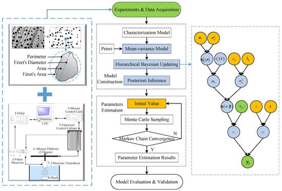
Figure 1.
(Color Online) Flow diagram of ultrasonic benchmarking for microstructure characterization using hierarchical Bayesian regression model. Note: The green containers represent the experimentally collected data; the orange containers represent their prior distributions that must be input during modeling; and the blue containers contain their posterior distributions that must be estimated.
For example, it is assumed that there are K1 types of experiment setups settings, K2 human factors, and K3 environmental factors for ultrasonic benchmarking. Thus, a total of sets of ultrasonic measurements for each benchmarking specimen should be undertaken, where nCr is the number of combination, n is the total number of elements in the set, and r is the number of elements chosen from this set. The measured microstructure parameter of the ith specimen in the kth () group is , and its mean value is calculated by the regression parameter array . In this study, we developed a hierarchical Bayesian regression model with a two-level structure using the aforementioned destructive and non-destructive data, where the base level’s regression parameters were utilized as the dependent variables for the second level. We assumed that could be determined by another hyperparameter array , i.e., a multi-dimensional joint prior to distribution could be used to describe the correlation between . As a result, by specifying a hyper-prior distribution for the hyperparameter , the Bayesian estimation of the regression parameter array could be implemented.
First, the first level of the hierarchical Bayesian regression model is [29]:
Next, all regression parameters at the first level were rewritten as dependent variables. We presumed that the intercept term α(k) at the first level had an mean term of and a random fluctuation of , and that the new intercept term and slope terms of at the second level were and . Similarly, the slope term at the first level was supposed to have an mean term of and a random fluctuation of , and that the new intercept term and slope terms of at the second level were and . Thus, the second level of the hierarchical model is [29]:
where are called the covariates. They serve as independent variables at the second level, assessing the difference of ultrasound characteristics of each group [29]. We assumed that the random fluctuations and followed a multidimensional joint normal distribution with zero means. Their covariance matrix is denoted by Cov, as [32]:
where the diagonal elements and are the variances of and , respectively. are the covariances between a and b (). Finally, substituting Equation (7) into (6), the hierarchical Bayesian regression model could be obtained as [29]:
On the right side of Equation (9), the first row represents the fixed-effects term, while the second row represents the random-effects term. Both are associated with the group number k, and the other terms without k communicate information between groups. As a result of communications, there is a distinction between developing a hierarchical model with k-groups and building k traditional models individually. This helps the model to take into account both the information about each group and the overall information, and to synthesize all the learned knowledge in order to effectively improve each group’s prediction accuracy.
Following the establishment of a hierarchical Bayesian regression model, the prior distributions of the parameters must be assumed, and the posterior distributions must be estimated. Among the several Bayesian parameter estimation strategies, the traditional Markov chain Monte Carlo approach can only find the optimal solution by random walk. However, the HMC algorithm is more efficient in analyzing the state space than the MCMC algorithm due to the application of the concept of dynamics in physical systems. In the next section, we will utilize the HMC algorithm to calculate the future states of the Markov chains in order to obtain faster convergence.
3. Experiments and Results
The study’s overall goal was to propose a gradual transition from destructive sampling inspection to non-destructive one-hundred-percent inspection through the use of long-term ultrasonic benchmarking with Bayesian updating. As an illustration, we reconstructed a classical application that characterized the nodularity of ductile iron. Although ultrasonic nodularity characterization was accomplished 40 years ago [35], it is still not widely available in the industrial applications (at least not in China’s factories). For this reason, we established a transition period and a long-term experiment during which destructive sampling inspections were continued and additional ultrasonic measurements were conducted. The ultrasonic benchmarking procedure was performed weekly, and data from the current week were utilized to update the model from the previous week. The transition period was sustained until the Bayesian estimation results were accurate enough to meet industrial requirements. In addition, the impact of experimental conditions on ultrasonic benchmarking was discovered. A series of damping levels were employed to reflect a variety of experimental setups. For human factors, inspectors with varied grades of expertise were engaged. Environmental factors were represented by varying electromagnetic noise levels. The detailed steps and results of the experiments are shown below.
3.1. Experimental Preparations
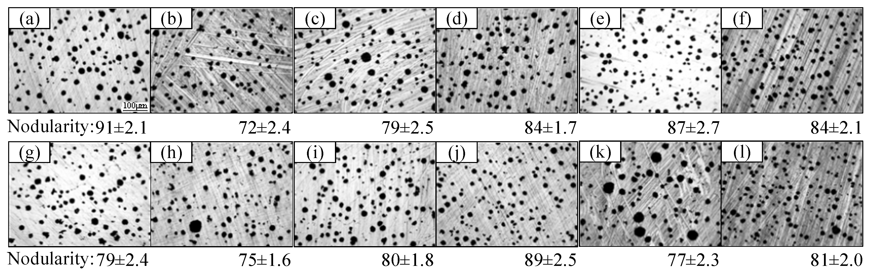
The chemical composition of ductile iron QT500-7 (China, GB) was (in wt.%): 3.60–3.80 C, 2.50–2.90 Si, Mn ≤ 0.60, P ≤ 0.08, S ≤ 0.025, and Fe, balance. Our experiment lasted for 13 weeks, from November 1st to January 30th. Weekly tests were conducted on ten benchmarking specimens (30 mm × 30 mm × 25 mm) cut from various portions of blanks and subjected to metallographic and ultrasonic measurements (12,000 mm × 2000 mm × 30 mm). After grinding and polishing, five metallographic images of each specimen were acquired using an Olympus optical microscope. The graphite particles in the metallographic images were then statistically measured to determine the nodularity [36]. For each benchmarking specimen, the mean value and standard deviation of the five metallographic images were used as the results of the destructive measurement. Figure 2a–j show the typical metallographic pictures and nodularity data for the benchmark specimens W1-1 to W1-10 during the first week. Additionally, two specimens, T-1 and T-2, were also prepared for the purpose of verifying the microstructure characterization results. Their microstructures are depicted in Figure 2k,l.
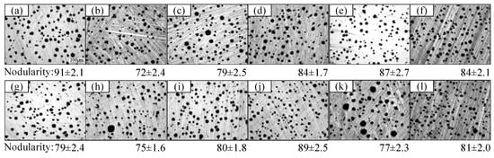
Figure 2.
The typical metallographic images and nodularity of specimens (%, Mean ± SD). (a–j) W1-1 to W1-10, (k) T-1, (l) T-2.
Next, water immersion ultrasonic measurements were performed on ten specimens every week. As shown in Figure 1, the ultrasonic system consisted of a JSR DPR 300 ultrasonic pulse generator/receiver (Imaginant Inc., Pittsford, NY, USA), a 200 MHz ADLINK PCIe-9852 DAQ card, an Olympus immersion transducer (I3-0508, 0.5 inch, 5 MHz, Olympus, Tokyo, Japan), and a computer-controlled micro-positioning system. A dual-mode ultrasonic velocity method was used to obtain the longitudinal wave velocity and transverse wave velocity [37]. A total of 12 groups of experimental conditions are shown in Table 1. Different damping levels were chosen since junior inspectors in the factory change the settings at whim. The maximum value, default value, and minimum value of damping in DPR 300 are 333, 49, and 25 Ohms, respectively. Consequently, we selected these three representative values for the experiments. Junior and senior inspectors were chosen based on their different operating skills and understanding of ultrasonic characterization. Different noise levels were chosen, owing to the inevitability of electromagnetic noise in the factory, and the likelihood that the double-shielded cable would be broken due to frequent use. Thus, a standard cable (with a high level of noise) and a double-shielded cable (with a low level of noise) were utilized to imitate this scenario.

Table 1.
Experiment conditions including different experimental setups, human factors, and environmental factors.
In addition, the Bayesian models in this study were mostly implemented using the BRMS package from Stan software (R package version 2.21.3). With the assistance of Stan software for HMC, a fast posterior distribution estimation for Equation (9) may be accomplished. Running the BRMS software in particular facilitates the rapid convergence of hierarchical model, regardless of whether the prior distributions are conjugated or not.
3.2. Results for First Week without Updating
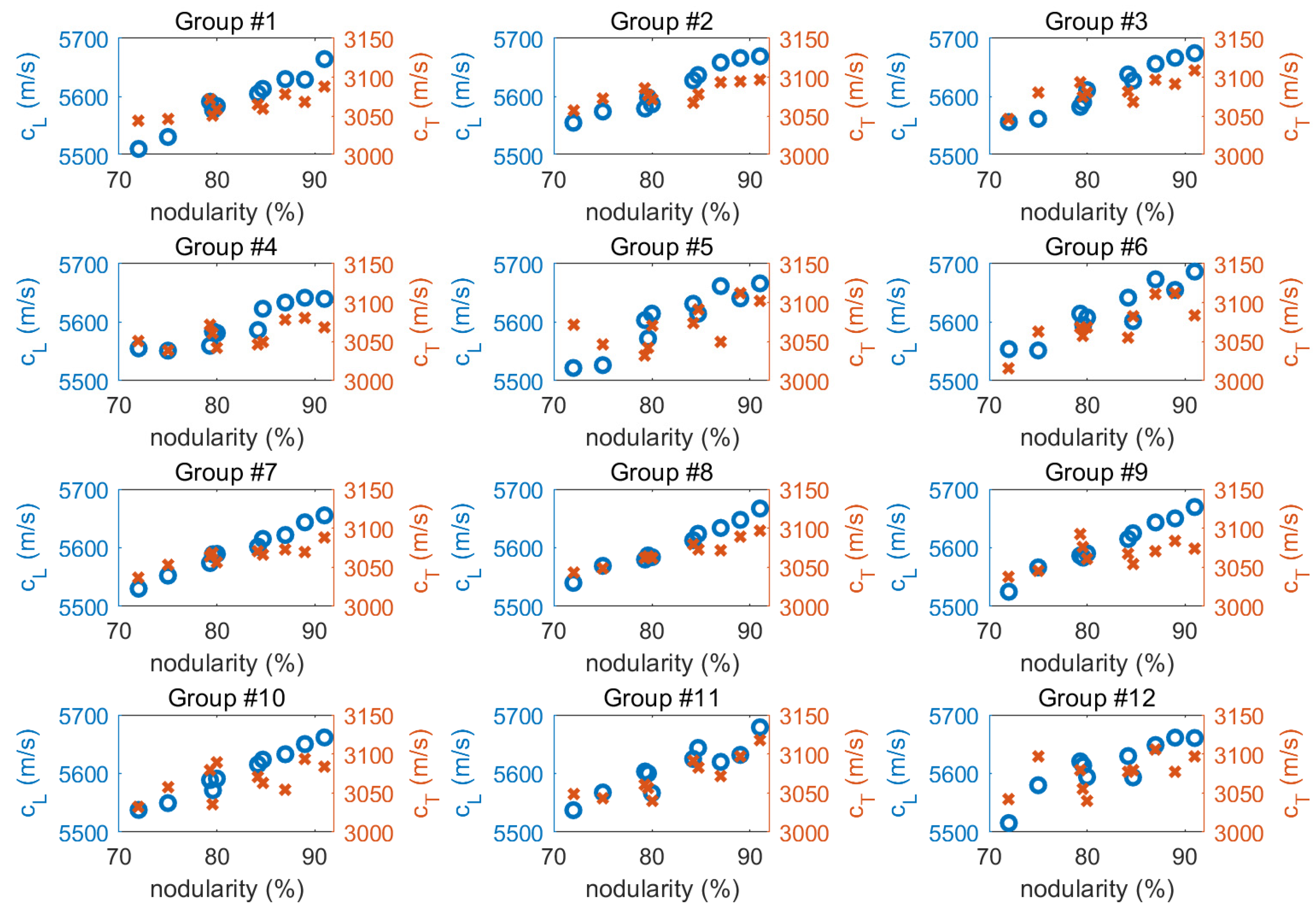
Figure 3 shows the relationships between nodularity, longitudinal wave velocity cL, and transverse wave velocity cT, based on 12 groups of experiments conducted on ten specimens during the first week. The results show that the nodularity was proportional to the cL and cT, which agreed with earlier experimental findings. An interesting finding was that the specific results from the 12 groups of experimental conditions varied slightly. When building a least-square fitting model or a traditional Bayesian regression model, certain users may ignore the impact of the experimental conditions. Therefore, we first built a traditional model by combining all of the data and then built a hierarchical model to see whether any discrepancies existed. The slope terms β1 and β2 of these two models are related to cL and cT in the following.
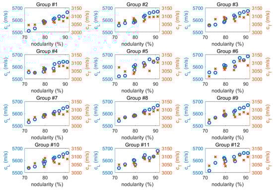
Figure 3.
(Color Online) Raw experimental data collected in the first week from ultrasonic measurements under different conditions. The longitudinal wave velocities are represented by blue circles, and the transverse wave velocities are represented by orange crosses.
3.2.1. Traditional Model
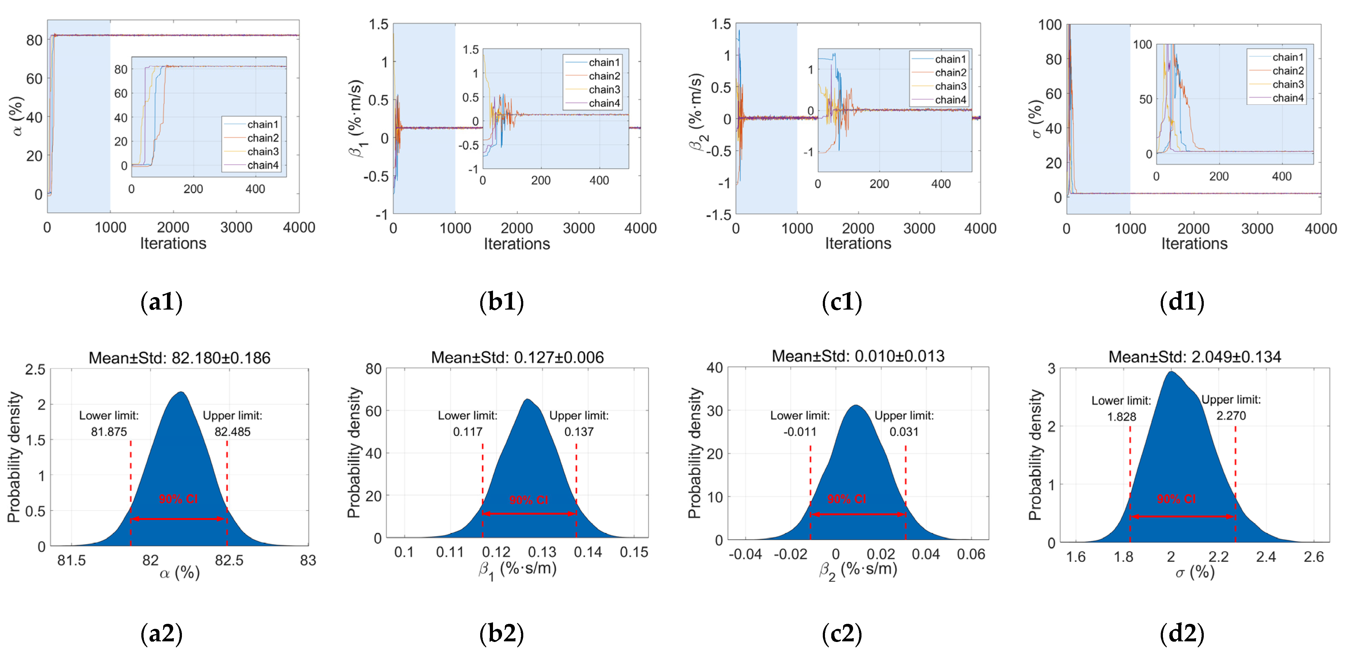
By mixing the 120 data points collected during the first week, a traditional Bayesian regression model was built. α, β1, β2, and σ were the parameters that were to be calculated. Four Markov chains were set up for each parameter, and each chain was iterated 4000 times, containing 1000 warm-up and 3000 actual sampling results. The four Markov chains for each parameter are shown in Figure 4a1–d1. Each chain began with varying values, but all the chains converged after the warm-up step (shown by the blue background). In terms of the kernel density estimation (KDE) for the actual sampling results of 4 × 3000 data [38], the posterior distributions of each parameter in the traditional model are shown in Figure 4a2–d2. From the posterior distributions, the mean, standard deviation, and 90% confidence bounds of each parameter can be indicated.

Figure 4.
(Color Online) Traditional Bayesian estimation results of parameters with data from the first week only. (a1–d1) Markov chains of parameters α, β1, β2, and σ, and (a2–d2) posterior distribution of parameters α, β1, β2, and σ.
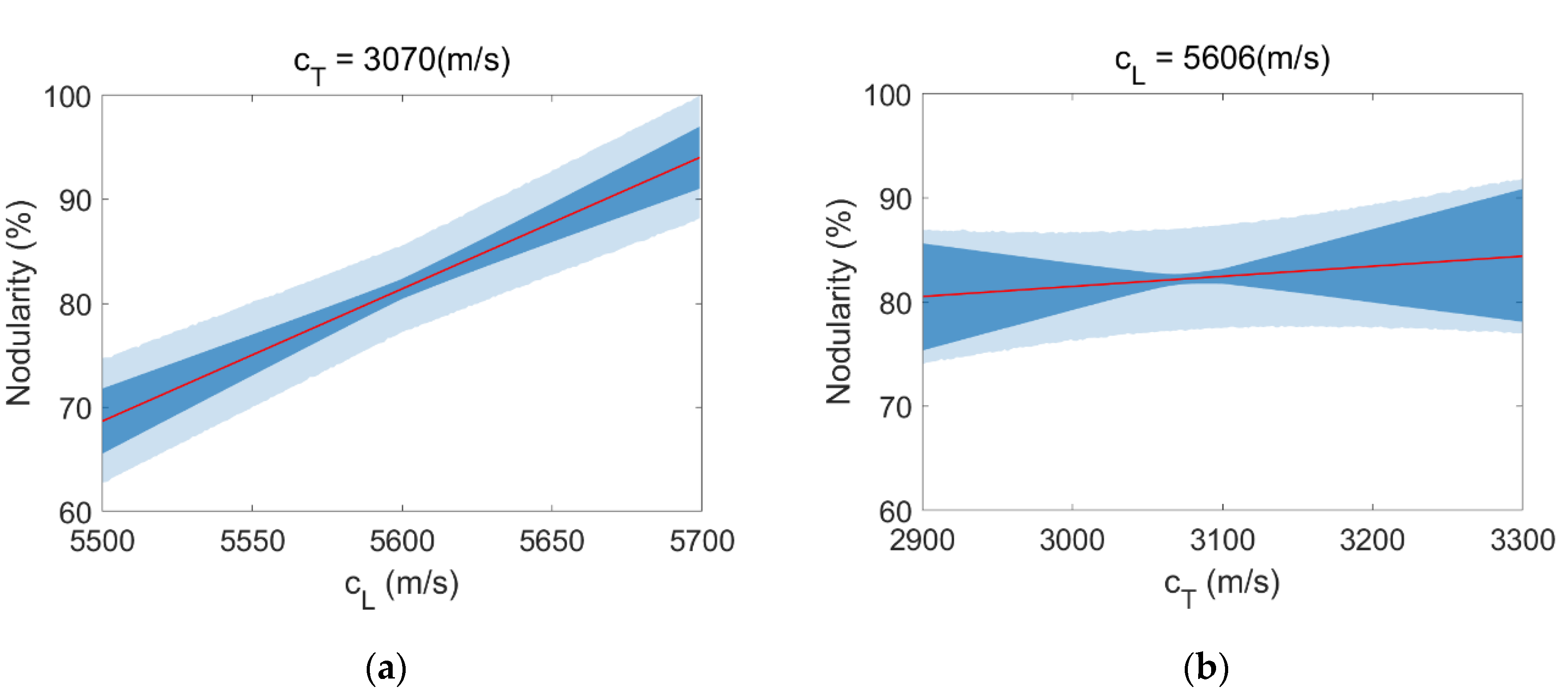
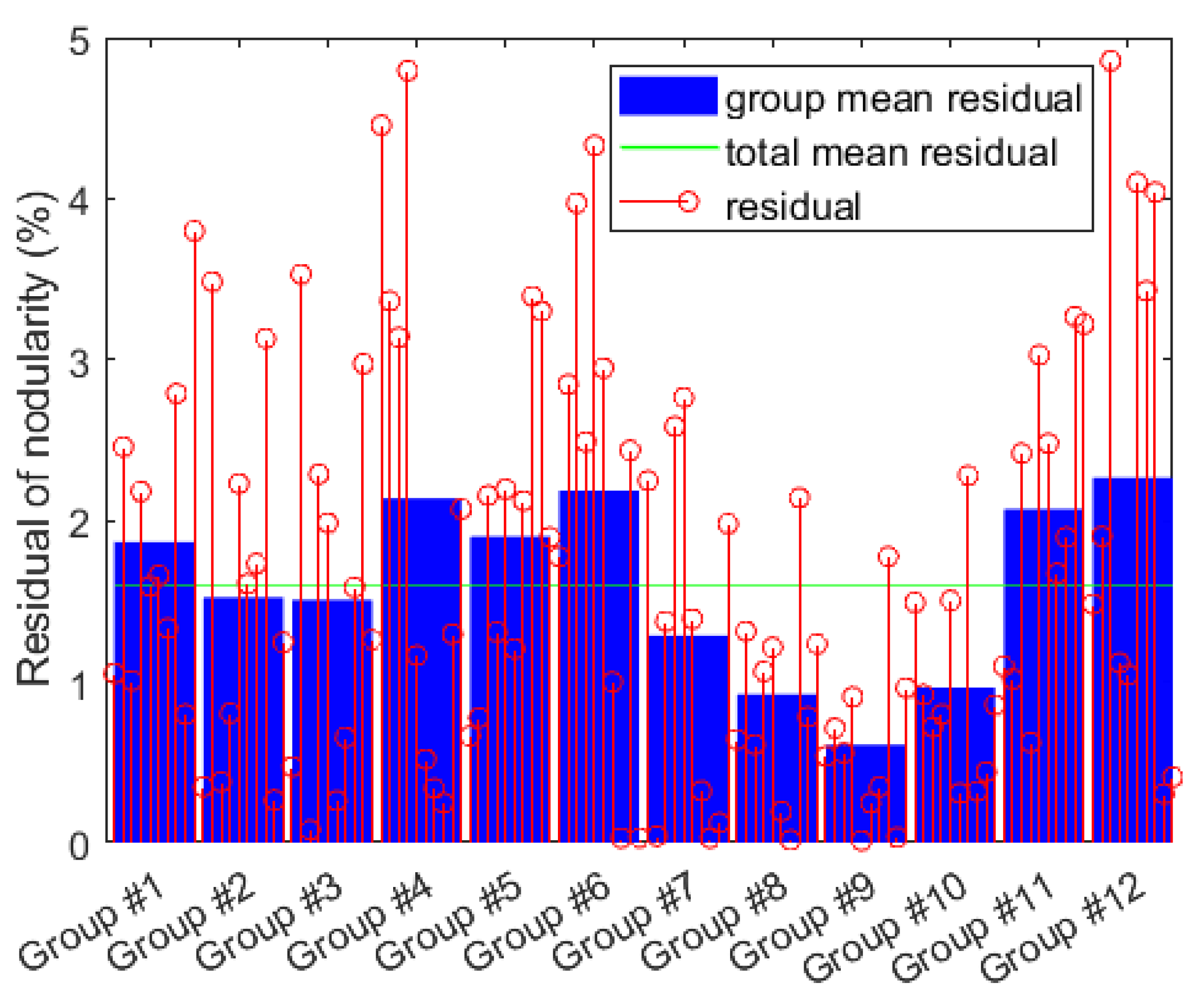
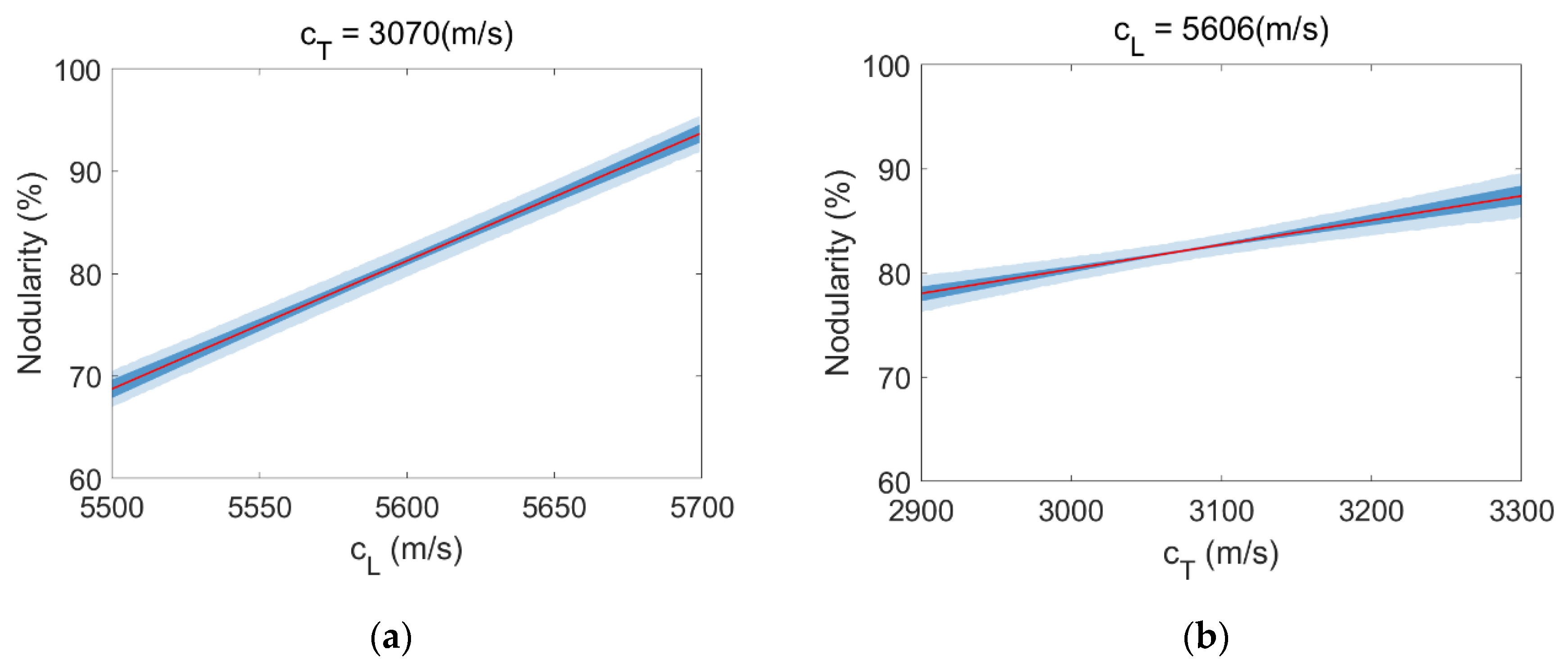
According to the posterior distribution of the parameters, the regression function and its associated confidence bounds can be obtained. Figure 5a,b show two cross-sections of the regression function used to characterize nodularity, one at cT = 3070 m/s and the other at cL = 5606 m/s, respectively. These two particular velocity values correspond to the mean values for cT and cL in the mixing dataset. The light blue areas illustrate the 90% confidence intervals for nodularity, the dark blue areas illustrate the 90% confidence intervals for the mean value of nodularity, and the red lines illustrate the mathematical expectations for the mean value of nodularity. To verify the model further, the residuals were calculated and analyzed as shown in Figure 6. The red bars represent the absolute values of the residual. The blue bars represent the mean of the red bars in each group, and the maximum deviation of group mean residual was 1.659% (between Group #9 and Group #12). The green line represents the mean of the blue bars, indicating that the total mean residual was 1.604%. Additionally, the residuals were all covered within the confidence intervals, shown by the light blue areas in Figure 5. In addition, the estimations of the nodularity of validation specimens T-1 and T-2 are shown in Section 3.3. Therefore, it is evident that the traditional Bayesian regression model’s estimation accuracy was low, the range of confidence intervals was large, and the model has to be optimized.
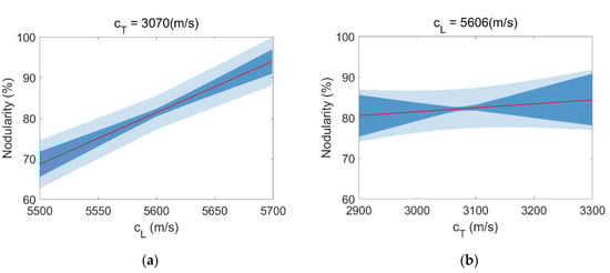
Figure 5.
(Color Online) The regression function and its associated 90% confidence bounds of traditional Bayesian regression model from the first week only. (a) A cross-section at cT = 3070 m/s, and (b) a cross-section at cL = 5606 m/s.

Figure 6.
(Color Online) The residual between the regression function and destructive data of traditional Bayesian regression model from the first week only.
3.2.2. Hierarchical Model
Next, the parameters of the hierarchical Bayesian regression model were estimated using 12 groups of experimental condition, including the fixed effect terms γα, , , να,1, να,2, , , , and , the random effect terms of second level σα, , , , , and , and the random effect term of base level σ. Four Markov chains were set up for each parameter as well, each with 4000 iterations (1000 warm-up and 3000 actual sampling).
The iterations of the Markov chain were plotted to examine if they converged, and some of the results are depicted in Figure 7. The results of Markov chain sampling for the parameters γα, να,1, , , σ, σα, , and are shown in Figure 7a1–h1. The associated posterior distributions are shown in Figure 7a2–h2, and we can see that the posterior distributions of the random effect terms of second level, such as σα, , and , were not normally distributed. The mean value, standard deviation, and 90% confidence interval for each parameter are given as shown in Table 2.
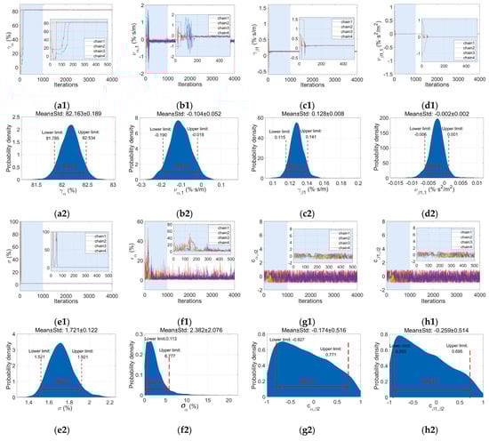
Figure 7.
(Color Online) Hierarchical Bayesian estimation results of parameters with data from the first week only. (a1–h1) Markov chains of parameters γα, να,1, , , σ, σα, , and . (a2–h2) Posterior distributions of parameters γα, να,1, , , σ, σα, , and .
Table 2.
The posterior distribution of hierarchical model parameters (without updating).
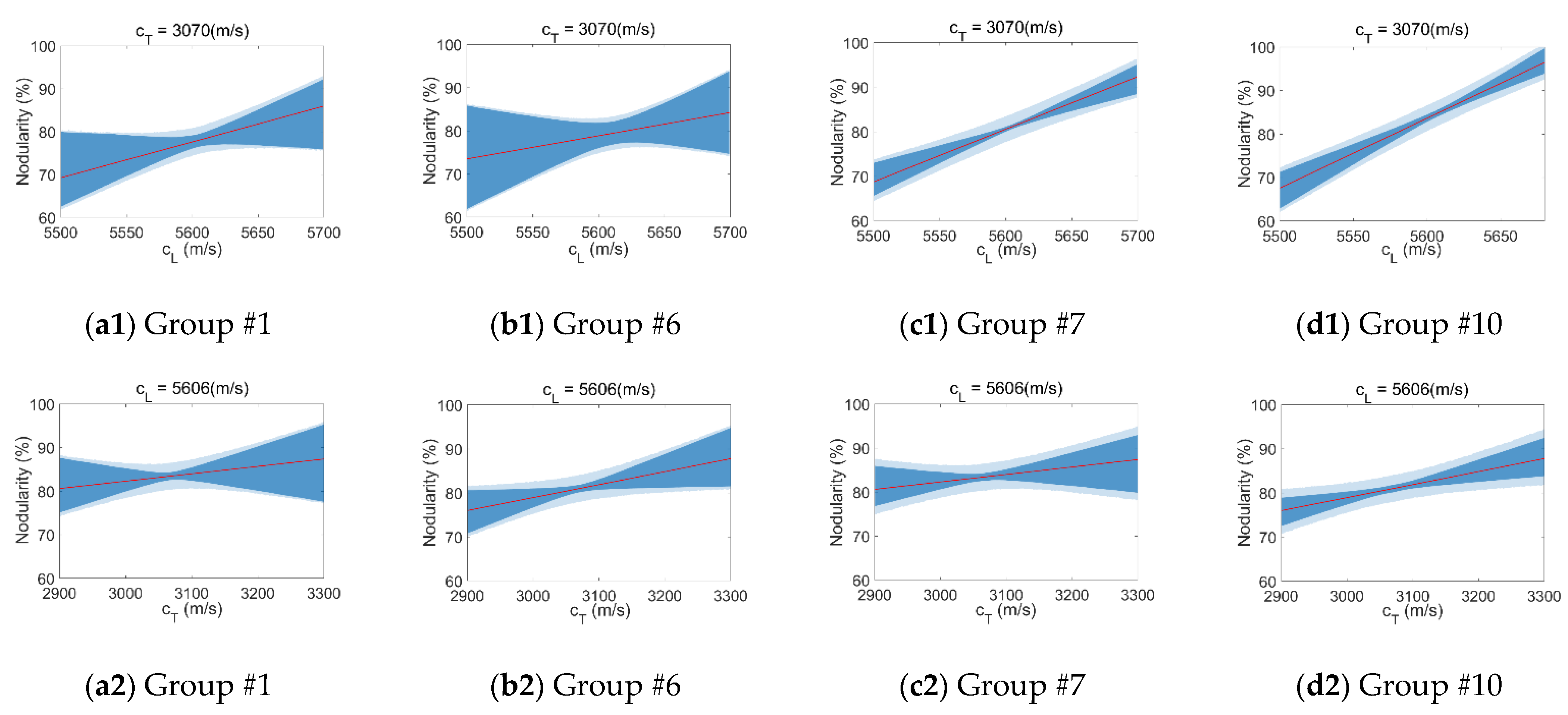
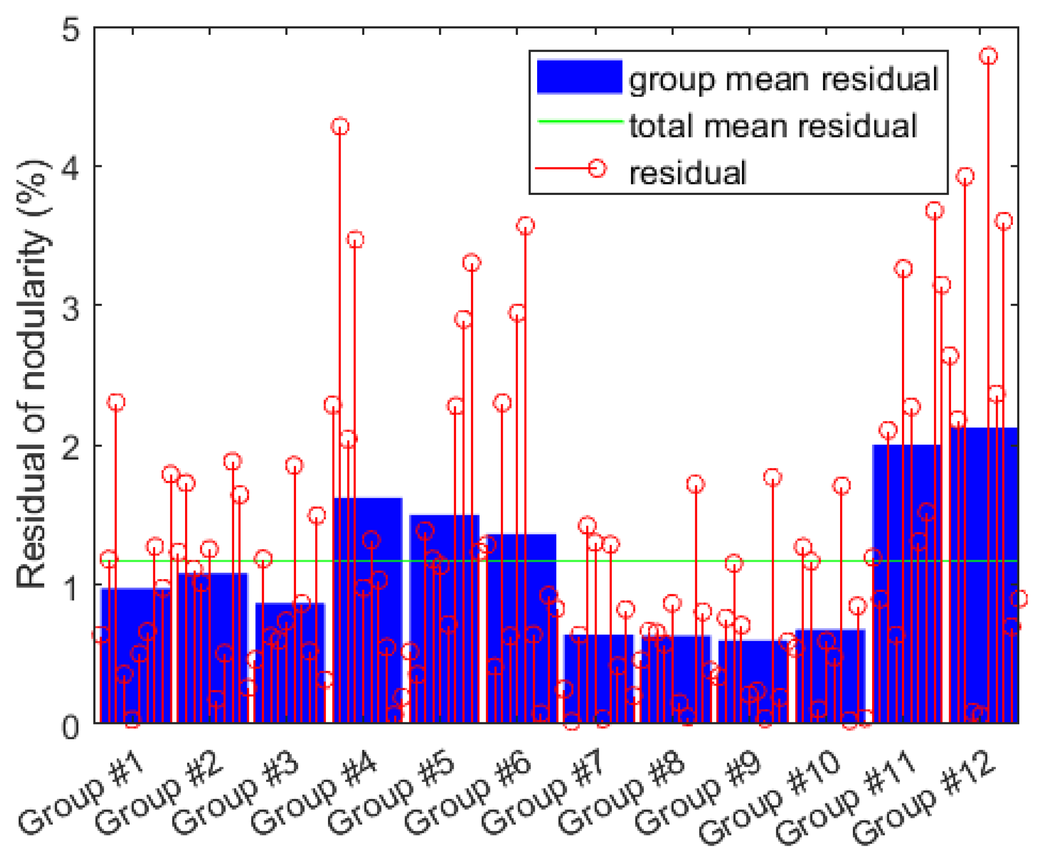
The preceding parameters’ estimation results were used to calculate the regression function and to characterize nodularity. Figure 8a1,a2, like Figure 5a,b, show two cross-section results of Group #1’s regression function, one at cT = 3070 m/s and the other at cL = 5606 m/s. Similarly, Figure 8b1,b2,c1,c2,d1,d2 correspond to Groups #6, #7, and #10. As noted, the confidence intervals for Groups #1 and #6 were rather large. This was because a higher level of electromagnetic noise led to in increased uncertainty, and the junior inspector was more likely to bias the experimental results. Furthermore, Figure 9 depicts the hierarchical model’s residuals. Both Groups #7 and #10 had relatively low residuals, indicating that the effects of damping setting on ultrasonic nodularity characterization were limited. Additionally, the hierarchical model’s total mean of residual was 1.175%, which is 0.429% lower than the total mean residual in the traditional model.

Figure 8.
(Color Online) The regression function and its associated 90% confidence bounds of hierarchical Bayesian regression model from the first week only. (a1–d1) Cross-sections at cT = 3070 m/s for Groups #1, #6, #7, and #10, and (a2–d2) cross-sections at cL = 5606 m/s for Groups #1, #6, #7, and #10.

Figure 9.
(Color Online) The residual between the regression function and destructive data of hierarchical Bayesian regression model from the first week only.
In addition, the model can be evaluated according to the information law, and the widely applicable information criterion (WAIC) is calculated as [39]:
where LPPD is the log pointwise predictive density, defined as the sum of the mean of likelihood corresponding to all observations, and pWAIC is the number of valid parameters obtained from the variance of the log-likelihood values of the observation. A small value for pWAIC indicates a simple model, while a large value for LPPD indicates an accurate model, implying that the WAIC evaluation is a balance between simplicity and accuracy. The WAIC value of a traditional Bayesian model is 515.1, but the WAIC value of a hierarchical Bayesian model is 488.3, demonstrating that the hierarchical model is more effective.
3.3. Results for Thirteen Weeks with Updating
3.3.1. Traditional Model
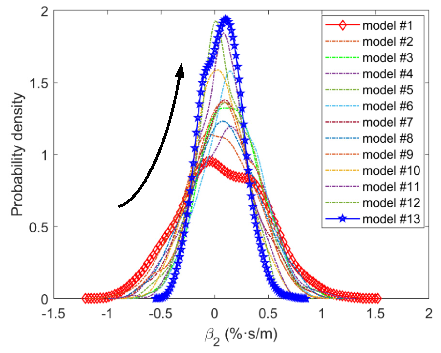
To update the original traditional model weekly, 120 benchmarking data of nodularity and ultrasonic longitudinal and transverse wave velocities were collected from ten benchmarking specimens using the aforementioned procedure. Figure 10 shows the evolution of the posterior distribution of parameter β2 from the first week to the thirteenth week. It can be seen that the standard deviation of posterior distribution of β2 gradually decreased as the sampling size of data increased with each model’s updating. Figure 10 shows the evolution of posterior distribution of parameter β2 from the first week to the thirteenth week. The standard deviation of the posterior distribution of β2 gradually decreased as the sample size of data increased with each updating. After a long-term Bayesian updating for the traditional model, the results of the regression function and its associated confidence bounds are shown in Figure 11, which still had two cross-sections. Compared with Figure 5, both the 90% confidence intervals for nodularity and the mean value of nodularity given by the updated model were significantly smaller, due to the larger sampling size of the input data. Because the experiment was repeated for three months, the long-term gage repeatability and reproducibility of the updated Bayesian model were superior to those of the non-updated Bayesian model, and that is self-evident.
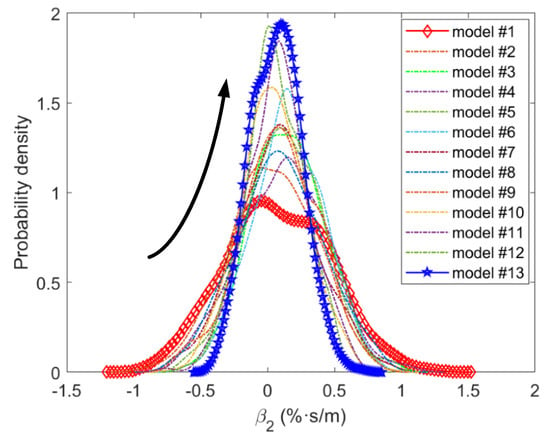
Figure 10.
(Color Online) The evolution of posterior distribution of parameter β2 from the first week to the thirteenth week.
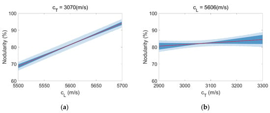
Figure 11.
(Color Online) The regression function and its associated 90% confidence bounds of traditional Bayesian regression model from the thirteenth week. (a) a cross-section at cT = 3070 m/s, (b) a cross-section at cL = 5606 m/s.
3.3.2. Hierarchical Model
Finally, we divided all of the benchmarking data into 12 groups depending on the different experimental conditions to update the hierarchical model. Based on a total of thirteen weeks of data, Figure 12 shows the best regression function and accompanying 90% confidence bounds from Group #7. The confidence intervals were noticeably smaller in comparison to Figure 8c1,c2 without updating. Table 3 summarizes the results of the nodularity estimation on validation specimens T-1 and T-2 using various methods, including the metallographic method, least-square fitting method of all data, traditional and hierarchical Bayesian regression models for the first week, traditional and hierarchical models for the sixth week, and traditional and hierarchical models for the thirteenth week. As can be seen, the least-square fitting approach was rarely used to determine the standard deviation and confidence interval for the estimated nodularity. The hierarchical model performed better than the traditional model, whether updated or not. When comparing the hierarchical models for the first, the sixth, and the thirteenth weeks, it was found that the updated model had improved accuracy and a reduced standard deviation. After long-term Bayesian updating, the confidence intervals got shorter, and the residual between the regression function and destructive metallographic observation could be described by the confidence intervals. In addition, the estimation results of the updated hierarchical model for the last week were comparable to the metallographic results, requiring the need for industrial application.
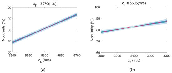
Figure 12.
(Color Online) The best regression function and its associated 90% confidence bounds of hierarchical Bayesian regression model of Group #7 from the thirteenth week. (a) A cross-section at cT = 3070 m/s, and (b) a cross-section at cL = 5606 m/s.
Table 3.
The estimation results of validation specimens T-1 and T-2 using different methods.
4. Conclusions
In this study, we proposed a long-term ultrasonic benchmarking method for microstructure characterization, along with a hierarchical Bayesian regression model, and analyzed the impacts of experimental setups, human factors, and environmental factors. The ultrasonic non-destructive characterization of the nodularity of cast iron was taken as an example. The benchmarking experiments were carried out over a transition period of 13 weeks. The results indicate that as the hierarchical model was considered the specialty of employing diverse experiment conditions, it worked better than the traditional Bayesian regression model, whether updated or not. Comparing the first-, sixth-, and thirteenth-weeks’ results, we observed that the updated hierarchical model had a more accurate mean value, a smaller standard deviation, and shorter confidence intervals. Moreover, the previous week’s updated hierarchical model provided comparable outcomes to the metallographic testing, bringing the transition period to an end. The proposed method was limited in that independent benchmarking and Bayesian updating were necessary for materials of varying grades, meaning that the regression models could not be transferred. In the next study, we will combine a Bayesian network with a transfer learning network to achieve ultrasonic benchmarking. We may also expand our method to characterize other microstructure parameters, such as the porosity of additive manufacturing materials, the content of second phase, and the grain size of polycrystals in the future.
Author Contributions
Data curation, F.Z.; formal analysis, F.Z.; investigation, F.Z.; software, F.Z.; validation, F.Z.; writing—original draft preparation, F.Z.; conceptualization, Y.S.; methodology, Y.S.; writing—review and editing, Y.S.; supervision, X.L. and P.N. All authors have read and agreed to the published version of the manuscript.
Funding
This research was funded by the National Natural Science Foundation of China, grant number 92060111.
Institutional Review Board Statement
Not applicable.
Informed Consent Statement
Not applicable.
Data Availability Statement
Due to the nature of this research, since the participants of this study did not agree for their data to be shared publicly, the supporting data are not available.
Conflicts of Interest
The authors declare no conflict of interest.
References
- Cui, C.Y.; Gu, Y.F.; Yuan, Y.; Osada, T.; Harada, H. Enhanced mechanical properties in a new Ni–Co base superalloy by controlling microstructures. Mater. Sci. Eng. A 2011, 528, 5465–5469. [Google Scholar] [CrossRef]
- Huang, H.; Talreja, R. Effects of void geometry on elastic properties of unidirectional fiber reinforced composites. Compos. Sci. Technol. 2005, 65, 1964–1981. [Google Scholar] [CrossRef]
- Kumar, A.S.; Kumar, B.R.; Datta, G.L.; Ranganath, V.R. Effect of microstructure and grain size on the fracture toughness of a micro-alloyed steel. Mater. Sci. Eng. A 2010, 527, 954–960. [Google Scholar] [CrossRef]
- Liang, C.; Ma, M.X.; Jia, M.T.; Raynova, S.; Yan, J.Q.; Zhang, D.L. Microstructures and tensile mechanical properties of Ti–6Al–4V bar/disk fabricated by powder compact extrusion/forging. Mater. Sci. Eng. A 2014, 619, 290–299. [Google Scholar] [CrossRef]
- Osório, W.R.; Freire, C.M.; Garcia, A. The role of macrostructural morphology and grain size on the corrosion resistance of Zn and Al castings. Mater. Sci. Eng. A 2005, 402, 22–32. [Google Scholar] [CrossRef]
- Epp, J. 4—X-ray diffraction (XRD) techniques for materials characterization. In Materials Characterization Using Nondestructive Evaluation (NDE) Methods; Hübschen, G., Altpeter, I., Tschuncky, R., Herrmann, H.-G., Eds.; Woodhead Publishing: Duxford, UK, 2016; pp. 81–124. [Google Scholar]
- Hübschen, G. 7—Ultrasonic techniques for materials characterization. In Materials Characterization Using Nondestructive Evaluation (NDE) Methods; Hübschen, G., Altpeter, I., Tschuncky, R., Herrmann, H.-G., Eds.; Woodhead Publishing: Duxford, UK, 2016; pp. 177–224. [Google Scholar]
- Inkson, B.J. 2—Scanning electron microscopy (SEM) and transmission electron microscopy (TEM) for materials characterization. In Materials Characterization Using Nondestructive Evaluation (NDE) Methods; Hübschen, G., Altpeter, I., Tschuncky, R., Herrmann, H.-G., Eds.; Woodhead Publishing: Duxford, UK, 2016; pp. 17–43. [Google Scholar]
- Pandey, D.; Pandey, S. Ultrasonics: A Technique of Material Characterization. In Acoustic Waves; IntechOpen: Rijeka, Croatia, 2010; pp. 397–398. [Google Scholar]
- Du, H.; Turner, J.A. Ultrasonic attenuation in pearlitic steel. Ultrasonics 2014, 54, 882–887. [Google Scholar] [CrossRef] [PubMed]
- Thompson, R.B.; Margetan, F.J.; Haldipur, P.; Yu, L.; Li, A.; Panetta, P.; Wasan, H. Scattering of elastic waves in simple and complex polycrystals. Wave Motion 2008, 45, 655–674. [Google Scholar] [CrossRef]
- Chassignole, B.; Duwig, V.; Ploix, M.A.; Guy, P.; El Guerjouma, R. Modelling the attenuation in the ATHENA finite elements code for the ultrasonic testing of austenitic stainless steel welds. Ultrasonics 2009, 49, 653–658. [Google Scholar] [CrossRef] [PubMed]
- Chimenti, D.E. Review of air-coupled ultrasonic materials characterization. Ultrasonics 2014, 54, 1804–1816. [Google Scholar] [CrossRef] [PubMed]
- Yap, Y.L.; Toh, W.; Koneru, R.; Chua, Z.Y.; Lin, K.; Yeoh, K.M.; Lim, C.M.; Lee, J.S.; Plemping, N.A.; Lin, R.; et al. Finite element analysis of 3D-Printed Acrylonitrile Styrene Acrylate (ASA) with Ultrasonic material characterization. Int. J. Comput. Mater. Sci. Eng. 2019, 08, 1950002. [Google Scholar] [CrossRef]
- Schmidt, J.; Marques, M.R.G.; Botti, S.; Marques, M.A.L. Recent advances and applications of machine learning in solid-state materials science. NPJ Comput. Mater. 2019, 5, 83. [Google Scholar] [CrossRef]
- Kushibiki, J.; Ono, Y.; Ohashi, Y. Experimental considerations on water-couplant temperature for accurate velocity measurements by the LFB ultrasonic material characterization system. In Proceedings of the 2000 IEEE Ultrasonics Symposium. Proceedings. An International Symposium (Cat. No.00CH37121), San Juan, PR, USA, 22–25 October 2000; Volume 1, pp. 619–623. [Google Scholar]
- Schmerr, L.W. Simulating the Experiments of the 2004 Ultrasonic Benchmark Study. AIP Conf. Proc. 2005, 760, 1880–1887. [Google Scholar]
- Song, S.J.; Schmerr, L.W., Jr.; Thompson, R.B. Ultrasonic Benchmarking Study: Overview Up to Year 2005. AIP Conf. Proc. 2006, 820, 1844–1853. [Google Scholar] [CrossRef]
- Liu, Y.; Kalkowski, M.K.; Huang, M.; Lowe, M.J.S.; Samaitis, V.; Cicėnas, V.; Schumm, A. Can ultrasound attenuation measurement be used to characterise grain statistics in castings? Ultrasonics 2021, 115, 106441. [Google Scholar] [CrossRef] [PubMed]
- Peng, S.; Chen, X.; Wu, G.; Li, M.; Chen, H. Ultrasound Evaluation of the Primary α Phase Grain Size Based on Generative Adversarial Network. Sensors 2022, 22, 3274. [Google Scholar] [CrossRef] [PubMed]
- Chen, J.; Liu, Y. Bayesian Information Fusion of Multmodality Nondestructive Measurements for Probabilistic Mechanical Property Estimation. In Proceedings of the ASME 2020 International Mechanical Engineering Congress and Exposition, Online, 16–19 November 2020. [Google Scholar]
- Guan, X.; Jha, R.; Liu, Y. Maximum Entropy Method for Model and Reliability Updating Using Inspection Data. In Proceedings of the AIAA 2010-2591. 51st AIAA/ASME/ASCE/AHS/ASC Structures, Structural Dynamics, and Materials Conference, Orlando, FL, USA, 12–15 April 2010. [Google Scholar]
- Guan, X.; Jha, R.; Liu, Y. Model selection, updating, and averaging for probabilistic fatigue damage prognosis. Struct. Saf. 2011, 33, 242–249. [Google Scholar] [CrossRef]
- Yang, J.; He, J.; Guan, X.; Wang, D.; Chen, H.; Zhang, W.; Liu, Y. A probabilistic crack size quantification method using in-situ Lamb wave test and Bayesian updating. Mech. Syst. Signal Processing 2016, 78, 118–133. [Google Scholar] [CrossRef]
- Zhang, Q.; Xu, N.; Ersoy, D.; Liu, Y. Manifold-based Conditional Bayesian network for aging pipe yield strength estimation with non-destructive measurements. Reliab. Eng. Syst. Saf. 2022, 223, 108447. [Google Scholar] [CrossRef]
- Tant, K.M.M.; Galetti, E.; Mulholland, A.J.; Curtis, A.; Gachagan, A. A transdimensional Bayesian approach to ultrasonic travel-time tomography for non-destructive testing. Inverse Probl. 2018, 34, 095002. [Google Scholar] [CrossRef] [Green Version]
- Bai, L.; Le Bourdais, F.; Miorelli, R.; Calmon, P.; Velichko, A.; Drinkwater, B.W. Ultrasonic Defect Characterization Using the Scattering Matrix: A Performance Comparison Study of Bayesian Inversion and Machine Learning Schemas. IEEE Trans. Ultrason. Ferroelectr. Freq. Control 2021, 68, 3143–3155. [Google Scholar] [CrossRef]
- Bai, L.; Zhang, J.; Velichko, A.; Drinkwater, B.W. The use of full-skip ultrasonic data and Bayesian inference for improved characterisation of crack-like defects. NDT E Int. 2021, 121, 102467. [Google Scholar] [CrossRef]
- Austin, P.; Goel, V.; van Walraven, C. An Introduction to Multilevel Regression Models. Can. J. Public Health 2001, 92, 150–154. [Google Scholar] [CrossRef] [PubMed]
- Aldrin, J.C.; Knopp, J.S.; Sabbagh, H.A. Bayesian methods in probability of detection estimation and model-assisted probability of detection evaluation. AIP Conf. Proc. 2013, 1511, 1733–1740. [Google Scholar] [CrossRef] [Green Version]
- Chiachío, J.; Bochud, N.; Chiachío, M.; Cantero, S.; Rus, G. A multilevel Bayesian method for ultrasound-based damage identification in composite laminates. Mech. Syst. Signal Processing 2017, 88, 462–477. [Google Scholar] [CrossRef] [Green Version]
- Bürkner, P.-C. brms: An R Package for Bayesian Multilevel Models Using Stan. J. Stat. Softw. 2017, 80, 1–28. [Google Scholar] [CrossRef] [Green Version]
- Gelman, A.; Carlin, J.; Stern, H.; Dunson, D.; Vehtari, A.; Rubin, D. Bayesian Data Analysis; Chapman and Hall/CRC: New York, NY, USA, 2013; pp. 16–31. [Google Scholar]
- Schneider, A.; Hommel, G.; Blettner, M. Linear regression analysis: Part 14 of a series on evaluation of scientific publications. Dtsch. Arztebl. Int. 2010, 107, 776–782. [Google Scholar] [CrossRef]
- Papadakis, E.P. Ultrasonic attenuation caused by Rayleigh scattering by graphite nodules in nodular cast iron. J. Acoust. Soc. Am. 1981, 70, 782–787. [Google Scholar] [CrossRef]
- ISO 945-4; Microstructure of Cast Irons—Part 4: Test Method for Evaluating Nodularity in Spheroidal Graphite Cast Irons. ISO: Geneva, Switzerland, 2019; p. 38.
- Liu, Y.; Song, Y.; Li, X.; Chen, C.; Zhou, K. Evaluating the reinforcement content and elastic properties of Mg-based composites using dual-mode ultrasonic velocities. Ultrasonics 2017, 81, 167–173. [Google Scholar] [CrossRef]
- Peter, D.H. Kernel estimation of a distribution function. Commun. Stat. —Theory Methods 1985, 14, 605–620. [Google Scholar] [CrossRef]
- Watanabe, S. Asymptotic Equivalence of Bayes Cross Validation and Widely Applicable Information Criterion in Singular Learning Theory. J. Mach. Learn. Res. 2010, 11, 3571–3594. [Google Scholar]


Publisher’s Note: MDPI stays neutral with regard to jurisdictional claims in published maps and institutional affiliations. |
© 2022 by the authors. Licensee MDPI, Basel, Switzerland. This article is an open access article distributed under the terms and conditions of the Creative Commons Attribution (CC BY) license (https://creativecommons.org/licenses/by/4.0/).