Abstract
This study presents a novel and thorough approach to comprehending and simulating the DRX process while hot compressing steel. To achieve this goal, we studied the high-temperature deformation behavior of a medium-carbon steel through hot compression testing on a Gleeble-3800 thermomechanical simulator over a broad range of strains, strain rates, and temperatures. We also employed an artificial neural network (ANN) to model the thermo-visco-plastic behavior with a flow law. The precision of quantifying the DRX volume fraction is dependent on critical conditions, which are essential for both analytical model evaluation and numerical implementation in finite element software. This study proposes a second ANN, serving as a universal approximator, to fit the data required for DRX critical condition calculations, whereas the Johnson–Mehl–Avrami–Kohnogorov (JMAK) model served as an analytical tool to estimate the DRX volume fraction, which underwent validation through experimental measurements. A numerical implementation of the JMAK model was conducted in ABAQUS software and compared against experimental data by means of microstructure analysis. The comparison revealed a strong correlation between the simulation and experiment. The study investigated the impact of temperature, strain, and strain rate on DRX evolution. The findings showed that DRX increases with rising temperature and strain but decreases with increasing strain rate.
1. Introduction
Dynamic recrystallization is a process observed in specific materials, mainly metals and alloys, as they undergo the process of plastic deformation. It is a phenomenon frequently seen in hot working operations, including hot rolling, hot forging, and hot extrusion. When a metal or alloy undergoes significant plastic deformation at high temperatures, its existing grain structure is disrupted. During the deformation process, new, smaller grains are formed, which is referred to as dynamic recrystallization (DRX). DRX differs from static recrystallization (SRX), which takes place when there is no deformation applied on the material. The amount of energy stored in the metal due to plastic deformation is the driving force behind the DRX process. Typically, the newly formed grains are much smaller than the original grains of the undeformed material. Their growth is accelerated by the stored energy and high temperatures. DRX provides several benefits in the hot forming process by refining the grain size and enhancing the mechanical properties of the material, including strength and toughness [1,2].
As the occurrence of DRX softens the material, the deformation loads during hot deformation must be adjusted from one pass to another to have a more accurate prediction of DRX. Therefore, understanding the critical conditions for dynamic recrystallization (DRX) is important for modeling industrial processes. However, the extent of DRX is influenced by factors such as material composition, deformation temperature, strain rate, and strain. By optimizing the parameters, engineers can attain the desired microstructures and mechanical properties in the final product. Various experimental techniques have been proposed by researchers to establish DRX’s critical conditions, such as metallographic analysis [3]. However, this technique requires extensive sampling before and after reaching the critical deformation point at which the material experiences recovery and recrystallization processes, resulting in the formation of new grains and a decrease in the average grain size. Additionally, the cooling phase sometimes entails phase changes (depending on the material’s type) from the hot working temperature, which alter the deformed structure, rendering the metallographic analysis complex. Hence, simpler techniques such as the development of analytical models are required to determine DRX initiation. In this regard, multiple studies have been carried out aiming to analytically identify the initiation of DRX. For instance, Yan Peng et al. [4] determined the critical strain and critical stress for DRX’s initiation based on the method proposed by Najafizadeh and Jonas [5] to establish a DRX kinetic model for hot-rolled conditions based on the relationship between the characteristic parameters of DRX and the temperature and strain rate. This approach defines the critical stress required for the initiation of DRX during deformation. According to Gottstein et al. [6], the critical strain for initiating DRX can also be predicted based on a work hardening model of dislocation density. The onset of dynamic recrystallization (DRX) may be identified through the inflection point in the strain hardening rate , where is the stress and is the strain.
The DRX phenomenon, based on the inflection point, was first studied by Ryan and McQueen [7,8,9]. They observed the appearance of an inflection point on the curve before the peak stress and attributed the beginning of DRX and the critical conditions to this point. Later, Poliak and Jonas [10,11,12,13] confirmed the hypothesis of DRX, describing the inflection point by demonstrating that it is associated with thermodynamic energy released during dislocation movements; the combination of the current dislocations with the previous one leads to DRX’s initiation. Najafizadeh and Jonas [5] simplified Poliak and Jonas’ thermodynamic model using an analytical technique to determine the critical conditions for initiating DRX. Their widely used approach relies on a third-degree polynomial to describe the curve and the second derivative to identify the critical stress and strain . Once calculated, the critical conditions serve as input data for the Johnson–Mehl–Avrami–Kolmogorov (JMAK) model [14]. This model is commonly used to estimate the volume fraction of dynamic recrystallization, , during hot working. Li et al. [15] investigated the DRX properties of micro-alloyed plastic molding steel by using the Avrami kinetics model equation and the Estrin and Mecking mathematical model [16,17] to determine the Avrami equation coefficients.
Zhang et al. [18] investigated the DRX behaviors of a medium-carbon alloy (Cr-Ni-Mo steel) using the Avrami kinetics model equation. They qualitatively characterized the alloy’s metallurgical properties based on variations in the Zener–Hollomon parameter. Cho et al. [19] and Razali et al. [20] used a well-established model to predict the microstructure evolution of a Mn alloy with a focus on DRX and grain growth phenomena. Their results showed consistency with multiple compression tests. Wan et al. [21] employed the same equation to predict the microstructure evolution of TiAl-based alloys during hot compression. Li et al. [22] validated the reliability of the Avrami kinetics model equation when testing the compression of Inconel 718 bolts. Cui et al. [23] analyzed DRX by applying the Avrami kinetics model equation and discovered that the -solidifying TiAl alloy usually started evolving at triple-joint boundaries before affecting the lamellae. Recently, Chen et al. [24] conducted a finite element analysis of DRX based on GCr15 (52100 steel) microstructure analysis and found that temperature and strain rate have a significant impact on DRX initiation.
The precision of the critical DRX conditions is closely linked to the method of obtaining the curve . Using experimental raw data directly does not yield functional curves; thus, smoothing the curve as much as possible or approximating it with a polynomial function that can reproduce the curve and deducing the curve from it is commonly used. The drawback of both of these methods is that they do not always ensure a satisfactory smoothing of the curve . Nevertheless, the universal approximator capability of artificial neural networks (ANN) has demonstrated effectiveness in various domains, such as predicting the flow behavior of materials, as in our previous work Tize Mha et al. [25] and many other works. Then, the predictions of are used as inputs for the prediction. Hence, this study offers a replacement of the two smoothing methods with an ANN approach to estimate the critical conditions for DRX.
2. Materials and Experiments
The experimental tests used in this work are identical to those previously published by Tize Mha et al. [25]. For additional information, readers can refer to the publications by our research group [26]. Nonetheless, we will outline the key aspects necessary to understand the suggested methodology.
2.1. Experimental Procedure and Compression Test Results
The material used for this study is a medium-carbon steel with the chemical composition presented in Table 1.

Table 1.
Chemical composition of medium-carbon steel. Fe = balance.
As detailed in Tize Mha et al. [25] and reported in Figure 1, hot compression tests were conducted on cylinders with an initial diameter of mm and a height of mm using a Gleeble-3800 thermomechanical simulator.
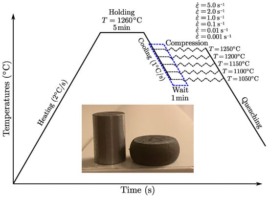
Figure 1.
Schematic diagram of the experimental process on the Gleeble-3800 thermomechanical simulator.
The tests were conducted at 5 temperature levels (ranging from 1050 to 1250 °C) and 6 strain rates (ranging from to ). The imposed displacement was set to mm, resulting in a reduction of of the initial height. To reduce friction during testing, thin tantalum sheets were used as a lubricant on the contact surface of the anvils and specimens. In order to remove thermal gradients, the samples were heated at a speed of 2 °C/s until they reached a temperature of 1260 °C, then held at that temperature for 5 min. They were subsequently cooled down to the test temperature at a speed of 1 °C/s and left at a consistent temperature for 1 min prior to being formed. During compression, the sample temperature was maintained at a constant level through the machine’s thermal control system. Subsequently, the structure was frozen at a fast pace in order to preserve the microstructure for future analysis.
The raw stress–strain data were exported from the Gleeble thermomechanical simulator as true stress and true strain, and the set of 30 flow stress curves versus strain obtained from compression tests for each test condition is reported in Figure 2. All stress–strain data are composed of 701 equidistant strain values from to in increments.
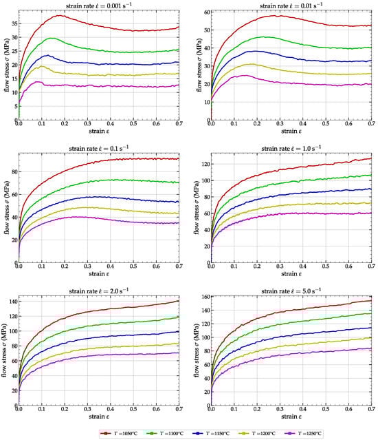
Figure 2.
Stress–strain curves of medium-carbon alloy extracted from the Gleeble device for 5 temperatures (T) and 6 strain rates ().
The flow stress () increases as the strain rate () rises but decreases as the temperature (T) increases. Notably, the strain also affects the flow stress. At the lowest strain rates, the flow stress increases up to as the strain approaches a value of about to . Then, it decreases to maintain a relatively constant value throughout the entire test. Conversely, at strain rates above , the flow stress increases steadily throughout the test. The nominal rise in stress observed at low strain rates with large strain values is attributed to friction between the sample and anvil during testing, as noted by Galos et al. [27]. Furthermore, this frictional effect becomes more apparent as lubrication reduces over time, as reported in Tize Mha et al. [25].
The initial increase in stress seen during deformation up to is believed to be due to work hardening (WH). Between and , the flow stress indicates a steady decrease as the stress level rises until a peak or inflection point is attained. This peak suggests that thermal softening is now the predominant influence, overtaking work hardening. At this stage, the stress–strain curve displays three distinct patterns as strain increases. The first pattern is a gradual decrease to a steady state with DRV/DRX softening, which is observed at all deformation temperatures and strain rates ranging from to , except at 1050 °C and 1100 °C. The second pattern is higher stress levels without significant softening and work hardening at 1050 °C and 1100 °C with a strain rate of . The last pattern is a continuous increase with significant work hardening observed for all deformation temperatures and a strain rate above . This indicates that DRX softening happens at high temperatures and low strain rates, and the rate of softening due to DRX slows down at higher strain rates and lower temperatures due to higher work hardening rates. The result is that both the peak stress and the onset of steady-state flow occur at higher strain levels. The decrease in stress detected across all temperatures and strain rates of is attributed to the event of dynamic recrystallization (DRX).
2.2. Identification of DRX Model’s Parameters
In this subsection we will determine the critical deformation required to initiate recrystallization. Ryan and McQueen [7,8,9] were the pioneers in investigating this phenomenon. Observing the appearance of an inflection point on the curve before the peak stress , the start of DRX was attributed to this inflection point and, therefore, the critical values of the strain () and stress (), respectively. Later, Poliak and Jonas [10,11,12,13] demonstrated that this inflection point is associated with a release of thermodynamic free energy during dislocation motion, supporting the DRX hypothesis. Najafizadeh and Jonas [5] developed an analytical technique to determine the critical conditions for DRX initiation, simplifying the thermodynamic model of Poliak and Jonas. Their widely used approach adopts a 3rd degree polynomial to describe the curve , enabling the identification of critical stress and strain ( and ) through the second derivative.
As previously stated, critical values for DRX initiation are determined by identifying the inflection point on the curve between and . One challenge is calculating the derivative of stress versus strain values numerically, as compression test data exhibit oscillations, as depicted in Figure 2. It is not feasible to compute the derivative directly.
To overcome this difficulty, certain authors propose smoothing out the empirical data (perhaps through the utilization of the Excel solver [5]) or discovering an analytical function (such as a polynomial with a relatively high degree) through a minimization algorithm. However, depending on the degree of the polynomial, for the same stress–strain curve, multiple solutions may be obtained. This results in multiple possible forms for the function.
2.2.1. ANN-Based Filtering Model’s Architecture
To improve the results obtained through the process of identifying critical values, we suggest employing the universal approximator capability of artificial neural networks. This can be done by characterizing each strain-hardening curve using an ANN with just one input (strain) and one output (stress). In this type of network, each layer of neurons is linked to the preceding and subsequent layers through weighted connections. Any hidden layer k, containing n neurons, takes a weighted sum of the outputs of the immediately preceding layer containing m neurons, given by the following equation:
where is the entry of the ith neuron of layer k, is the output of the jth neuron of layer , is the associated weight parameter between the ith neuron of layer k and the jth neuron of layer , and is the associated bias of the ith neuron of layer k. Those weights and bias , for each layer, are the training parameters of the ANN, which we have to adjust during the training procedure. For the proposed model, we selected the Sigmoid activation function, so that each neuron in the hidden layer k provided an output value from the input value y of the same neuron defined by Equation (1) according to the following equation:
No activation function was used for the output neuron of the ANN, as is typically omitted in regression applications. The chosen architecture for our application consists of two hidden layers, one with 7 neurons and the other with 5 neurons, as illustrated in Figure 3. To calculate the number of internal parameters in the model, where n and m represent the number of neurons in the first and second hidden layers, respectively, the following formula may be used: .
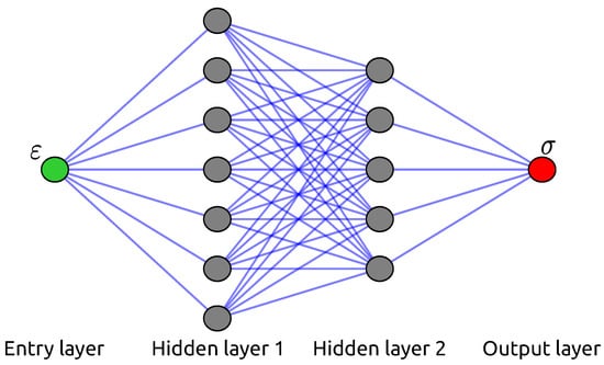
Figure 3.
Two-hidden-layer artificial neural network architecture with 1 input neuron (green) and 1 output neuron (red).
Thus, for a 7-5 network, .
The Python program used for training the neural network was created with the dedicated Python library, Tensorflow [28]. The training phase employed the Adaptive Moment Estimation (ADAM) optimizer [29]. The training was conducted using 50,000 epochs of the experimental dataset. It took approximately 15 min to train the ANN model and obtain the converged parameters on a Dell XPS-13 7390 laptop running Ubuntu 22.04 LTS 64-bit with 16 GB of RAM and an Intel 4-core i7-10510U processor.
2.2.2. ANN-Based Filtering Model’s Application
Since the dynamic recrystallization phenomenon only occurs for strain rates between and , we used only the first 20 stress–strain curves to identify the critical DRX parameters. Each of these 20 curves consisted of 701 pairs of strain–stress values and was independently processed by a neural network, resulting in the identification of 20 networks. As an example, Figure 4 displays the stress–strain curve experimental values for and °C (in blue) and the neural network results identified from these data (in red).
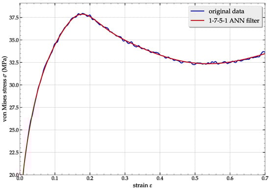
Figure 4.
Filtering of the stress–strain data using the ANN for and °C.
A models’ accuracy and predictive ability are typically evaluated using specific coefficients, such as the mean absolute relative error (), as defined by the following equation:
and the root-mean-squared error (), as defined by the following equation:
where is the experimental value, is the value of the stress predicted using the given model, and N is the total number of data points used to compute those coefficients. For the proposed ANN filter, and , while using a 11th order polynomial fit of the experimental data leads to and .
It is evident that using the ANN model to depict the curve is superior to using an 11th-order polynomial fit, as demonstrated by the lower estimated error. Thus, this architecture of the ANN model is used for all subsequent curves, resulting in the deduction of the hardening curves, which illustrates the stress change rate relative to the strain (). An illustration of computing the hardening curve for a single temperature is displayed in Figure 5. The blue line represents the direct calculation of the derivative of the raw stress versus strain, whereas the red line represents the derivative of the stress filtered by the neural network versus strain. An overview of the remaining temperatures can be found in Figure 6. The identical process applies to all 20 stress–strain curves. These curves deliver essential data regarding the critical stresses and strains required for predicting DRX in the subsequent analysis.
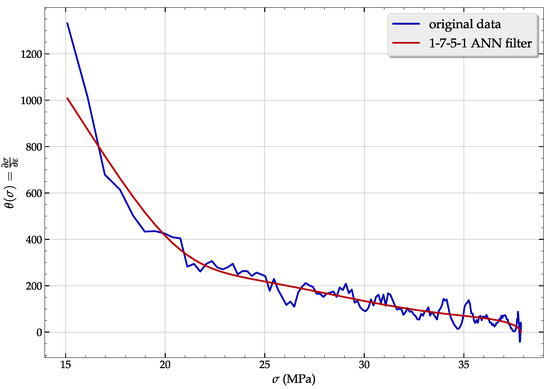
Figure 5.
Computation of the hardening curve from the stress–strain data using the ANN for and °C.
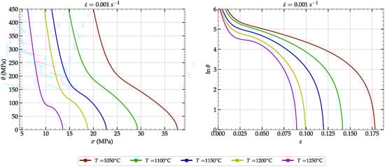
Figure 6.
Work hardening computation for one strain rate and five temperatures.
2.2.3. Evaluation of the Critical Conditions
As described previously, dynamic recrystallization only occurs when a particular critical condition is met. The identification of these critical conditions is a difficult task that calls for the creation of models that can compute the corresponding critical stress and strain. Consequently, the Poliak and Jonas [10,11,12,13] method, which is currently well-regarded, will be used in this investigation. The method uses a third-degree polynomial function to describe the and curves reported in Figure 6 for . The objective is to locate the inflection points connected to the critical stress and critical strain , as well as to extract the peak stress and peak strain from those curves.
The determination of critical values is carried out in two consecutive steps for each of the curves. Firstly, based on the definition of the curve as depicted in Figure 6, we use the polyfit method from the numpy library to determine the optimal values of the constants for a third-degree polynomial function approximating :
Secondly, the inflection point can be obtained from the second derivative of with:
Similarly, the critical strain () is calculated by defining a third-degree polynomial function approximating the curve as depicted in Figure 6:
This later gives the critical strain from . Applying the identical method to the first four strain rates and all temperatures, Table 2 summarizes the critical stress and strain, peak stress, and peak strain. Once the critical DRX conditions are established, they can be used as input to determine the DRX volume fraction, which will be discussed in the following section.
Table 2.
Critical conditions based on the proposed approach.
2.3. Evaluation of the DRX Model’s Parameters
The DRX process commences at a critical deformation, as previously noted. The degree of recrystallization can be determined through experimental means. For a visual representation of microstructure evolution during DRX, the interested reader can refer to Chen et al. [30].
The flow stress curve of the material is influenced by the rate of work hardening, which in turn is affected by dislocations within the free grains. The predicted volume fraction of the dynamic recrystallization () is estimated using the Avrami model [14], commonly known as the JMAK model, expressed by the following equation:
with and as the critical and peak strain, respectively. k and are the model’s parameters, and the experimental equivalence of this volume fraction of DRX is given by
where and are the peak stress and the steady stress after the peak stress, respectively. The steady stress is considered the minimum value after the peak stress. It is possible to establish a dependency relationship between these specific stresses and strains and the Zener–Hollomon [31] parameter , (where Q is the effective activation energy parameter and R is the universal gas constant ), according to the following equation reported by other researchers such as [32,33,34] for similar steel compositions and deformation conditions:
with the parameters , , , , , , , , , and , which are the specific strains and stresses’ dependency on the Zener–Hollomon parameter, whose identification is described hereafter. The procedure for determining the value of Q is detailed in [25].
The JMAK model’s parameter identification involves two main steps, starting with determining the 10 coefficients A, n, B, and m. Secondly, those coefficients are integrated into Equation (10) to be used in Equations (8) and (9). To calculate these parameters, the curve_fit method of the scipy library is employed through a Python code. These parameter identifications use the critical strains and stresses computed in the preceding sections as input data. The curve-fitting method seeks to obtain optimal values for the coefficients by iteratively adjusting them to minimize the gap between predicted and actual critical strains and stresses. This optimization process entails experimenting with different combinations of coefficients and assessing their appropriateness for the provided data. The curve-fitting technique fine-tunes coefficients until it attains the most accurate match between the model’s forecasts and the experimental data.
Once the calculation of the constants that define the dependency of the Zener–Hollomon parameter is completed, an optimization technique can be employed to deduce the JMAK model parameters while minimizing the error between the predicted recrystallization and the experimental value . Table 3 displays the dependency of both the Zener–Hollomon parameters and the JMAK model’s parameters.
Table 3.
JMAK model and Zener–Hollomon dependency parameters.
The critical conditions calculated by the Poliak method are used to provide the curves of in Figure 7, where a comparison between the experimental and predicted values is made for the strain rate and three temperatures (1050 °C, 1150 °C and 1250 °C).
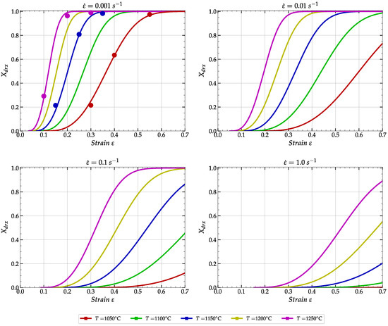
Figure 7.
DRX experimental data (dots) and JMAK model-based prediction (plain lines).
Figure 8 shows a micrograph of the sample for , T = 1050 °C, and . From this, we determined the location of one experimental point in Figure 7 (the red one for ). The same approach using different temperatures and strains was used to obtain the other experimental points reported in Figure 7.
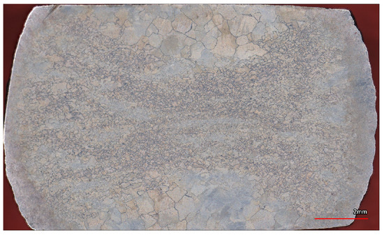
Figure 8.
Micrograph of the sample for , °C, and .
The curves illustrate the changes in the predicted volume fractions of DRX with plastic strain, and it is evident that the proportion of DRX is strongly affected by strain, temperature, and strain rate values. The DRX kinetics exhibit an S-shaped curve, with the DRX volume fraction gradually increasing with strain. At a constant temperature and strain, the DRX volume fraction increases with decreasing strain rate. Conversely, at a fixed strain rate and strain, the DRX volume fraction increases with rising temperature. The difference between the predicted and experimental volume fractions of DRX is insignificant, confirming the suitability of the proposed approach for DRX prediction in the studied superalloy under various forming conditions. The reduction in DRX with increasing strain rate can be attributed to the sensitivity of the volume fraction of dynamic recrystallization to the forming temperature and strain rate. Dynamic recrystallization is prone to occur at high forming temperatures and low strain rates due to increased grain boundary mobility. However, because of the limited mobility of grain boundaries, the rate of dynamic recrystallization is slow at low forming temperatures and high strain rates. The validation of the model used in the study, as evidenced by the correlation between experimental and predicted results, supports the subsequent use of these findings in the simulation section.
3. Numerical Simulation of the Compression
In this section, we will focus on numerically validating the previously performed identification of dynamic recrystallization. This requires establishing a constitutive law capable of accurately predicting the material’s plastic deformation. In our previous publication (Tize Mha et al. [25]), we conducted a comparison between analytical constitutive laws and a neural network-based approach. The results revealed an artificial neural network model as the most appropriate option for this material. As a result, this section has two main focuses: first, a summary of the ANN-based constitutive law identification, as previously presented; and second, the incorporation of this identified ANN model with the JMAK model to predict dynamic recrystallization behavior.
3.1. Identification of the ANN Constitutive Law
In general terms, flow stress is a non-linear function of the strain , increasing with the strain rate but decreasing with increasing temperature T. This model can be described as an elastoplastic model that takes into consideration the influence of temperature and strain rate. This type of behavior generally leads to Johnson–Cook [35], Zerilli–Armstrong [36], Hansel–Spittel [37], PTM [25], or Arrhenius [38] flow law type. Depending on the nature of the stress–strain relationship, modeling with one or another of these models can take into account the actual behavior of the material at certain strain rates.
As stated in the research conducted by Tize Mha et al. [25], the Johnson–Cook, Zerilli–Armstrong, or Hansel–Spittel models provide an estimate of material behavior at strain rates exceeding , but they neglect the softening due to DRX that is evident on experimental curves for strain rates below , as presented in Figure 2. Indeed, at the lowest strain rates, the flow stress increases with strain until it reaches a value of roughly to . Afterward, it decreases, maintaining a relatively constant value until the end of the compression test. The Arrhenius model is the only one that can somewhat explain this softening at low strain rates. As proposed by Pantalé et al. [26] and Tize Mha et al. [25], an effective alternative is to use a flow law defined by an artificial neural network trained directly on experimental data from compression tests. Properly defining the hyper-parameters of this neural network, such as the number of hidden layers, number of neurons, and activation functions, enables us to obtain a flow law that accurately replicates the data acquired from compression tests.
According to the method proposed by Pantalé et al. [26], we have developed a two-hidden-layer artificial neural network-based flow law in Tize Mha et al. [25]. Figure 9 shows the general structure of this ANN. The input layer of the ANN consists of three neurons that correspond to the model inputs, which are , , and T. The output layer of the ANN contains one neuron representing , while there are two hidden layers. All details regarding the artificial neural network, experimental data setup, and training method are detailed in the paper proposed by Pantalé et al. [26].
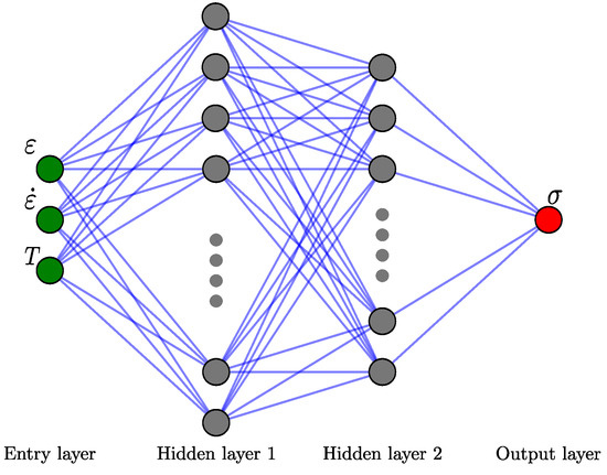
Figure 9.
Two-hidden-layer artificial neural network architecture with 3 inputs neurons (green) and 1 output neuron (red).
We again used the Tensorflow library to develop the training program and employed the ADAM optimizer for the training phase. The training database, as described in Section 2.1, contains 21,030 quadruples (we have quadruples because with an increment of , so we have 701 values and 30 data curves) of values for strain (), strain rate (), temperature (T), and stress ().
We selected six different networks, named 3-n-m-1, where n represents the number of neurons in the first hidden layer and m indicates the number of neurons in the second hidden layer, to demonstrate the significance of choosing the appropriate number of neurons in these two layers.
The training was conducted based on 5000 epochs of the experimental dataset. It took 40 min to train the ANN model and obtain the converged parameters on a Dell XPS-13 7390 laptop running Ubuntu 22.04 LTS 64-bit operating system with 16 GB of RAM and an Intel 4-core i7-10510U processor.
Figure 10 shows the evolution of the training error, defined by the of the internal , during the training phase. Table 4 summarizes the final values of this criterion, as well as the final values of the and the for all six neural network configurations. Based on these results, the 3-15-7-1 network was chosen for further investigation. This network exhibited the most efficient convergence and achieved the lowest final error values of and while also maintaining a reasonable number of internal parameters (). The global performance of the model is illustrated in Figure 11.
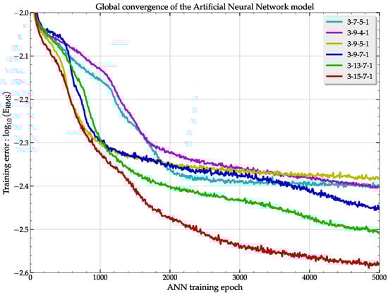
Figure 10.
Evolution of the convergence of the models during the training procedure for the 6 proposed network architectures.
Table 4.
Architecture and accuracy coefficients for all the proposed networks.
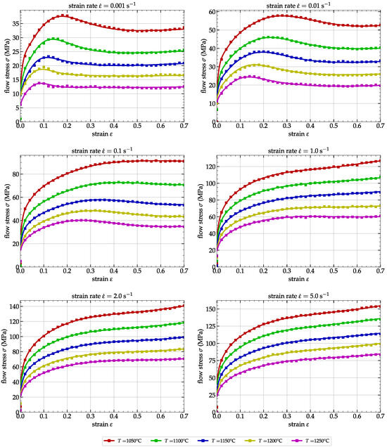
Figure 11.
Comparison between the experimental (dots) and predicted (lines) flow stresses by the 3-15-7-1 ANN model.
This model will serve as the material flow equation for the numerical simulations discussed in Section 3.2. Once the neural network was trained and a stable solution was obtained, it was re-implemented as a Fortran 77 VUHARD subroutine to calculate the material flow stress in the Abaqus FEM code. The details of the procedure and complete equation set required to calculate the flow stress and the three derivatives of the flow stress with respect to , , and T can be found in [26].
3.2. Dynamic Recrystallization Simulation
To evaluate the effectiveness of the DRX model presented earlier, we propose a numerical simulation of a compression test in this section. Our simulation concerns a medium-carbon P20 iron alloy, the same material used for the model’s identification. An axisymmetric finite element (FE) model of hot cylinder compression with a height of mm and a diameter of mm was used, as shown in Figure 12. The assumed friction coefficient at the material/die interface was [39,40]. The mesh was composed of 986 () CAX4R elements (4-node axisymmetric bi-linear quadrilateral elements with reduced integration and hourglass control). Abaqus/Implicit was used to run the FE model simulation because of the long time needed to simulate a low strain rate compression. A displacement of and of the total height was imposed on the upper part of the cylinder along the vertical axis of the specimen during compression. The upper and the lower parts of the specimen can slip in the radial direction according to the friction coefficient and the contact conditions. The axial displacement () of the upper part was imposed with a fixed velocity, while the axial displacement of the lower part remained fixed during the simulation. The simulation evaluated the impact of reducing the cylinder height on the effects of strain rate and temperature. Conclusions were drawn based on this analysis. The simulation considered three temperatures (1050 °C, 1150 °C, and 1250 °C) and four strain rates (, , , and ).
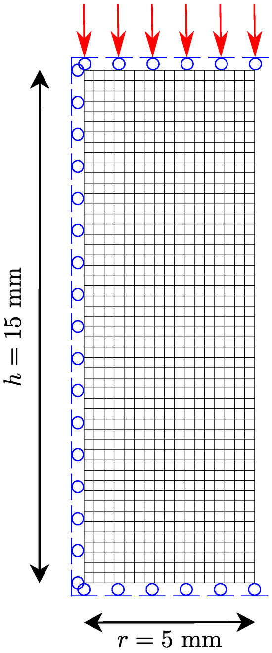
Figure 12.
Numerical FE model for the simulation of the compression test.
3.2.1. Temperature and Strain Rate Effects
Temperature and strain rate are critical factors that influence dynamic recrystallization in materials, particularly metals and alloys. This process leads to the formation of new grains within the material. Higher temperatures and lower strain rates typically result in increased nucleation rates and faster growth rates of new grains during dynamic recrystallization. Conversely, lower temperatures and higher strain rates can lead to incomplete dynamic recrystallization. At high temperatures, the increased mobility of both atoms and dislocations facilitates the formation of fresh grain boundaries and promotes the growth of new grains, resulting in a more refined and isotropic grain structure. In addition, higher temperatures can raise the proportion of recrystallized material, with the enhanced dislocation mobility contributing to new grain creation. Consequently, this may result in a substantial change in the microstructure and the mechanical properties of the material. Figure 13 and Figure 14 display the simulated results of the DRX fraction of P20 steel under different deformation conditions. Figure 13 shows that as the temperature increases, the extent of dynamic recrystallization widens. The gradual increase in the dynamic recrystallization fraction in the center is noticeable, spreading outward. This expansion is a result of higher thermal activation and increased atomic diffusion at higher temperatures, which makes the material more vulnerable to dynamic recrystallization. The dynamic recrystallization degree () unequivocally grows with the increase in temperature and reduction. At and reduction, the of P20 steel attained in the center of the specimen at all the initial sample temperatures. Indeed, the plastic deformation of a material is accompanied by the creation of dislocations. These dislocations represent a “storage of elastic energy”. When the temperature is high enough, the dislocations become spontaneously mobile and cause a reorganization of the crystal structure in two stages: restoration and recrystallization. The nature of the phases remains unchanged (those that are thermodynamically stable), and the atoms retain the same lattice. However, the grain boundaries and the orientation of the crystallites undergo changes.
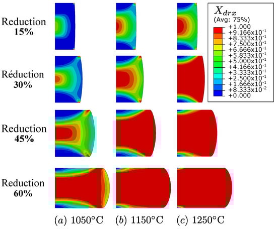
Figure 13.
values at a fixed strain rate of for different reductions and initial temperatures .
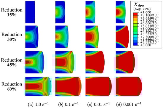
Figure 14.
values at a fixed °C for different reductions and strain rates.
The temperature at which these phenomena occur depends on the rate of deformation. The amount of elastic energy stored by a material increases with the degree of deformation, initiating restoration and recrystallization at a lower temperature. As shown in Figure 14, escalating strain rates result in a decrease in the extent of recrystallization due to reduced dynamic recrystallization magnitude. This result is due to the faster strain rate, which increases the critical strain and decreases the chance of internal dynamic recrystallization in the material.
3.2.2. Comparison with Some Experiments
In this section, we will compare experimental and simulation data by observing the dynamic recrystallization percentage of selected regions. Figure 15 shows a comparison between experimental data and simulation data for a test conducted at a temperature of 1150 °C with a strain rate of . Four zones were chosen to observe the percentage of recrystallization, ranging from to . The corresponds to the dead zone, representing the contact area between the sample and die experiencing friction effects. In contrast, corresponds to the value observed at the center of the sample, where deformation is the highest. The temperature is elevated at the center of the sample, leading to a significant accumulation of energy. Conversely, at the edges of the sample, a relatively complete recrystallization is observed. This is because the temperature during deformation shifts from the center towards the upper and lower regions of the piece (due to the fact that the anvils are cooled), allowing recrystallization to occur. Microscopic observations of each zone show large grains (Figure 15d) in the dead zone, while small grains (Figure 15a) are observed in the center of the sample, resulting from complete recrystallization.
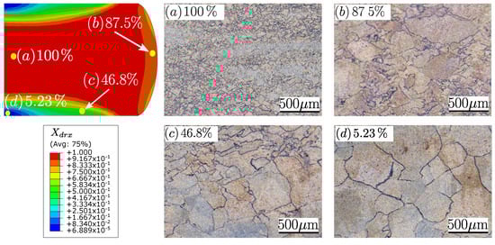
Figure 15.
Experimental and numerical values for °C and strain rate .
Figure 16 shows a comparison of the numerical results for a strain rate , an initial temperature °C, and a reduction of (i.e., ) and its comparison with the microstructure obtained experimentally for the same conditions after an interrupted test with the same reduction level. It can be seen later that there is a correspondence between the fully recrystallized area in the center of the sample (the red zone in the numerical simulation) and the corresponding zone where the microstructure has changed in the center of the sample, promoting a labrys (a double-edged) axe shape. As can be clearly seen on the micrograph, recrystallization is not complete in the areas of contact with the upper and lower anvils, where the numerical value of is less than and the microstructure enhances very large grains. We can also see on the microstructure that recrystallization is not complete along the periphery of the cylinder, where the numerical value of is in the range of 75 to .
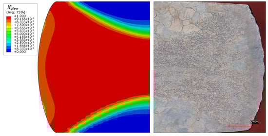
Figure 16.
Comparison of the micrography and numerical values for °C, strain rate , and reduction ().
4. Conclusions
In this study, we used the abilities of the ANN technique to deeply comprehend the dynamic recrystallization process and its adaptations in varying conditions. Through the fusion of ANN modeling, fundamental material models, simulation software, and experimental confirmation, a comprehensive framework has been created that greatly enhances the materials science and engineering fields. Initially, we successfully used an ANN model to efficiently filter flow stress curves, which enabled us to predict critical conditions using the Poliak model. This allowed us to accurately anticipate the conditions at which the DRX process begins, providing a valuable tool for predicting material behavior under specific deformation scenarios.
We used the predicted critical conditions as input into the JMAK model, resulting in the successful prediction of the volume fraction of DRX and providing valuable insights into the kinetics and mechanisms controlling recrystallization. This incorporation establishes a connection between theoretical models and practical phenomena, ultimately leading to a more deep comprehension of the complex processes occurring during deformation. Taking our investigation further, we integrated the JMAK model into the widely used ABAQUS software to simulate the evolution of DRX during hot compression tests. This allowed us to capture the process’s response to varying conditions without bias. By comparing our simulation results with experimental data and using microstructure analysis, we have validated the accuracy of our simulations and confirmed the effectiveness of our predictive models.
It is noteworthy that although our research represents a significant milestone, it also presents opportunities for future exploration. Further enhancing the accuracy and applicability of our predictions can be achieved by fine-tuning our model, expanding our dataset, and refining the integration process. Moreover, the successful connection of theory, simulation, and experimentation offers a sturdy structure for addressing challenging material behavior issues in industries ranging from manufacturing to aerospace or other applications.
Author Contributions
Conceptualization, P.T.M. and O.P.; methodology, O.P.; software, P.T.M. and O.P.; validation, O.P.; formal analysis, O.P. and P.D.; investigation, P.D.; resources, P.D. and M.J.; data curation, P.T.M. and P.D.; writing—original draft preparation, O.P. and P.T.M.; writing—review and editing, O.P.; visualization, O.P.; supervision, M.J., A.T. and O.P.; project administration, M.J.; funding acquisition, M.J. All authors have read and agreed to the published version of the manuscript.
Funding
This work was supported by the Natural Sciences and Engineering Research Council of Canada (NSERC) in the framework of a Collaborative Research and Development project (CRD) (Grant Number 5364418).
Data Availability Statement
The raw/processed data required to reproduce these findings cannot be shared at this time due to privacy and ethical concerns.
Acknowledgments
The authors acknowledge Jean-Benoit Morin, Director of Metallurgy and Quality from Finkl Steel-Sorel, Abdelhalim Loucif from the R&D department of Finkl Steel-Sorel, Ecole de Technologie Superieure, and Ecole Nationale d’Ingenieurs de Tarbes, France, for providing technical data, materials, and testing facilities.
Conflicts of Interest
The authors declare no conflict of interest.
Abbreviations
The following abbreviations are used in this manuscript:
| ANN | Artificial neural network |
| DRX | Dynamic recrystallization |
| DRX’s volume fraction: for experimental and predicted values, respectively | |
| FE | Finite element |
| SRX | Static recrystallization |
| WH | Work hardening |
References
- Javidikia, M.; Sadeghifar, M.; Champliaud, H.; Jahazi, M. Grain size and temperature evolutions during linear friction welding of Ni-base superalloy Waspaloy: Simulations and experimental validations. J. Adv. Join. Process. 2023, 8, 100150. [Google Scholar] [CrossRef]
- Shen, J.; Zhang, L.; Hu, L.; Sun, Y.; Gao, F.; Liu, W.; Yu, H. Effect of subgrain and the associated DRX behaviour on the texture modification of Mg-6.63 Zn-0.56 Zr alloy during hot tensile deformation. Mater. Sci. Eng. A 2021, 823, 141745. [Google Scholar] [CrossRef]
- Babu, K.A.; Mozumder, Y.H.; Athreya, C.N.; Sarma, V.S.; Mandal, S. Implication of initial grain size on DRX mechanism and grain refinement in super-304H SS in a wide range of strain rates during large-strain hot deformation. Mater. Sci. Eng. A 2022, 832, 142269. [Google Scholar] [CrossRef]
- Peng, Y.; Guo, S.; Liu, C.; Barella, S.; Liang, S.; Gruttadauria, A.; Mapelli, C. Dynamic recrystallization behavior of low-carbon steel during hot rolling process: Modeling and simulation. J. Mater. Res. Technol. 2022, 20, 1266–1290. [Google Scholar] [CrossRef]
- Najafizadeh, A.; Jonas, J.J. Predicting the critical stress for initiation of dynamic recrystallization. ISIJ Int. 2006, 46, 1679–1684. [Google Scholar] [CrossRef]
- Gottstein, G.; Frommert, M.; Goerdeler, M.; Schäfer, N. Prediction of the critical conditions for dynamic recrystallization in the austenitic steel 800H. Mater. Sci. Eng. A 2004, 387, 604–608. [Google Scholar] [CrossRef]
- Ryan, N.D.; McQueen, H.J. Dynamic recovery, strain hardening and flow stress in hot working of 316 steel. Czechoslov. J. Phys. B 1989, 39, 458–465. [Google Scholar] [CrossRef]
- Ryan, N.D.; McQueen, H.J. Dynamic softening mechanisms in 304 austenitic stainless steel. Can. Metall. Q. 1990, 29, 147–162. [Google Scholar] [CrossRef]
- Ryan, N.D.; McQueen, H.J. Flow stress, dynamic restoration, strain hardening and ductility in hot working of 316 steel. J. Mater. Process. Technol. 1990, 21, 177–199. [Google Scholar] [CrossRef]
- Poliak, E.I.; Jonas, J.J. A one-parameter approach to determining the critical conditions for the initiation of dynamic recrystallization. Acta Mater. 1996, 44, 127–136. [Google Scholar] [CrossRef]
- Poliak, E.I.; Jonas, J.J. Initiation of dynamic recrystallization in constant strain rate hot deformation. ISIJ Int. 2003, 43, 684–691. [Google Scholar] [CrossRef]
- Poliak, E.I.; Jonas, J.J. Critical strain for dynamic recrystallization in variable strain rate hot deformation. ISIJ Int. 2003, 43, 692–700. [Google Scholar] [CrossRef]
- Jonas, J.J.; Poliak, E.I. The critical strain for dynamic recrystallization in rolling mills. In Materials Science Forum; Trans Tech Publications Ltd.: Stafa-Zurich, Switzerland, 2003; Volume 426, pp. 57–66. [Google Scholar] [CrossRef]
- Avrami, M. Kinetics of Phase Change. I General Theory. J. Chem. Phys. 1939, 7, 1103–1112. [Google Scholar] [CrossRef]
- Li, X.; Duan, L.; Li, J.; Wu, X. Experimental study and numerical simulation of dynamic recrystallization behavior of a micro-alloyed plastic mold steel. Mater. Des. 2015, 66, 309–320. [Google Scholar] [CrossRef]
- Estrin, Y.; Mecking, H. A unified phenomenological description of work hardening and creep based on one-parameter models. Acta Metall. 1984, 32, 57–70. [Google Scholar] [CrossRef]
- Mecking, H.; Kocks, U.F. Kinetics of flow and strain-hardening. Acta Metall. 1981, 29, 1865–1875. [Google Scholar] [CrossRef]
- Zhang, C.; Zhang, L.; Xu, Q.; Xia, Y.; Shen, W. The kinetics and cellular automaton modeling of dynamic recrystallization behavior of a medium carbon Cr-Ni-Mo alloyed steel in hot working process. Mater. Sci. Eng. A 2016, 678, 33–43. [Google Scholar] [CrossRef]
- Cho, J.R.; Jeong, H.S.; Cha, D.J.; Bae, W.B.; Lee, J.W. Prediction of microstructural evolution and recrystallization behaviors of a hot working die steel by FEM. J. Mater. Process. Technol. 2005, 160, 1–8. [Google Scholar] [CrossRef]
- Razali, M.K.; Joun, M.S. A new approach of predicting dynamic recrystallization using directly a flow stress model and its application to medium Mn steel. J. Mater. Res. Technol. 2021, 11, 1881–1894. [Google Scholar] [CrossRef]
- Wan, Z.; Sun, Y.; Hu, L.; Yu, H. Experimental study and numerical simulation of dynamic recrystallization behavior of TiAl-based alloy. Mater. Des. 2017, 122, 11–20. [Google Scholar] [CrossRef]
- Li, C.; Tan, Y.; Zhao, F. Finite element simulation and process optimization of microstructure evolution in the formation of Inconel 718 alloy bolts. Mater. Res. Express 2018, 6, 026578. [Google Scholar] [CrossRef]
- Cui, N.; Kong, F.; Wang, X.; Chen, Y.; Zhou, H. Hot deformation behavior and dynamic recrystallization of a β-solidifying TiAl alloy. Mater. Sci. Eng. A 2016, 652, 231–238. [Google Scholar] [CrossRef]
- Chen, X.; Sun, J.; Yang, Y.; Liu, B.; Si, Y.; Zhou, J. Finite Element Analysis of Dynamic Recrystallization Model and Microstructural Evolution for GCr15 Bearing Steel Warm–Hot Deformation Process. Materials 2023, 16, 4806. [Google Scholar] [CrossRef]
- Tize Mha, P.; Dhondapure, P.; Jahazi, M.; Tongne, A.; Pantalé, O. Interpolation and Extrapolation Performance Measurement of Analytical and ANN-Based Flow Laws for Hot Deformation Behavior of Medium Carbon Steel. Metals 2023, 13, 633. [Google Scholar] [CrossRef]
- Pantalé, O.; Tize Mha, P.; Tongne, A. Efficient implementation of non-linear flow law using neural network into the Abaqus Explicit FEM code. Finite Elem. Anal. Des. 2022, 198, 103647. [Google Scholar] [CrossRef]
- Galos, J.; Das, R.; Sutcliffe, M.P.; Mouritz, A.P. Review of balsa core sandwich composite structures. Mater. Des. 2022, 221, 111013. [Google Scholar] [CrossRef]
- Abadi, M.; Barham, P.; Chen, J.; Chen, Z.; Davis, A.; Dean, J.; Devin, M.; Ghemawat, S.; Irving, G.; Isard, M.; et al. TensorFlow: A System for Large-Scale Machine Learning. In Proceedings of the 12th USENIX Conference on Operating Systems Design and Implementation, Savannah, GA, USA, 2–4 November 2016; pp. 265–283. [Google Scholar]
- Kingma, D.P.; Lei, J. Adam: A method for stochastic optimization. arXiv 2015, arXiv:1412.6980. [Google Scholar] [CrossRef]
- Chen, X.; Zhang, J.; Du, Y.; Wang, G.; Huang, T. Dynamic Recrystallization Simulation for X12 Alloy Steel by CA Method Based on Modified L-J Dislocation Density Model. Metals 2019, 9, 1291. [Google Scholar] [CrossRef]
- Zener, C.; Hollomon, J.H. Effect of strain rate upon plastic flow of steel. J. Appl. Phys. 1944, 15, 22–32. [Google Scholar] [CrossRef]
- Chen, X.M.; Lin, Y.; Wen, D.X.; Zhang, J.L.; He, M. Dynamic recrystallization behavior of a typical nickel-based superalloy during hot deformation. Mater. Des. 2014, 57, 568–577. [Google Scholar] [CrossRef]
- Li, L.; Wang, Y.; Li, H.; Jiang, W.; Wang, T.; Zhang, C.C.; Wang, F.; Garmestani, H. Effect of the Zener-Hollomon parameter on the dynamic recrystallization kinetics of Mg–Zn–Zr–Yb magnesium alloy. Comput. Mater. Sci. 2019, 166, 221–229. [Google Scholar] [CrossRef]
- Wang, T.; Chen, Y.; Ouyang, B.; Zhou, X.; Hu, J.; Le, Q. Artificial neural network modified constitutive descriptions for hot deformation and kinetic models for dynamic recrystallization of novel AZE311 and AZX311 alloys. Mater. Sci. Eng. A 2021, 816, 141259. [Google Scholar] [CrossRef]
- Johnson, G.R.; Cook, W.H. A constitutive model and data for materials subjected to large strains, high strain rates, and high temperatures. In Proceedings of the 7th International Symposium on Ballistics, Hague, The Netherlands, 19–21 April 1983; pp. 541–547. [Google Scholar] [CrossRef]
- Zerilli, F.J.; Armstrong, R.W. Dislocation-mechanics-based constitutive relations for material dynamics calculations. J. Appl. Phys. 1987, 61, 1816–1825. [Google Scholar] [CrossRef]
- Hensel, A.; Spittel, T. Kraft- und Arbeitsbedarf Bildsamer Formgebungsverfahren; Deutscher Verlag für Grundstoffindustrie: Leipzig, Germany, 1978. [Google Scholar]
- Sellars, C.M.; McTegart, W.J. On the mechanism of hot deformation. Acta Metall. 1966, 14, 1136–1138. [Google Scholar] [CrossRef]
- Zhang, M.; Sun, X.; Wang, Y. Elevated temperature deformation characteristics of 15Mn7 steels. Procedia Manuf. 2019, 37, 360–366. [Google Scholar] [CrossRef]
- Sun, X.; Zhang, M.; Wang, Y.; Sun, Y.; Wang, Y. Kinetics and numerical simulation of dynamic recrystallization behavior of medium Mn steel in hot working. Steel Res. Int. 2020, 91, 1900675. [Google Scholar] [CrossRef]


Disclaimer/Publisher’s Note: The statements, opinions and data contained in all publications are solely those of the individual author(s) and contributor(s) and not of MDPI and/or the editor(s). MDPI and/or the editor(s) disclaim responsibility for any injury to people or property resulting from any ideas, methods, instructions or products referred to in the content. |
© 2023 by the authors. Licensee MDPI, Basel, Switzerland. This article is an open access article distributed under the terms and conditions of the Creative Commons Attribution (CC BY) license (https://creativecommons.org/licenses/by/4.0/).