Article

Determination of Vickers Hardness in D2 Steel and TiNbN Coating Using Convolutional Neural Networks

by
Juan C. Buitrago Diaz
1,2,
Carolina Ortega-Portilla
3,
Claudia L. Mambuscay
1,2,
Jeferson Fernando Piamba
1,2 and
Manuel G. Forero
4,*
1
Semillero Lún, Facultad de Ingeniería, Universidad de Ibagué, Ibagué 730002, Colombia
2
Semillero NOVAMAT, Facultad de Ciencias Naturales y Matemáticas, Universidad de Ibagué, Ibagué 730002, Colombia
3
CONAHCYT-Centro de Ingeniería y Desarrollo Industrial (CIDESI), Av. Playa, Av. Pie de la Cuesta No. 702, Desarrollo San Pablo, Santiago de Querétaro 76125, Mexico
4
Professional School of Systems Engineering, Faculty of Engineering, Architecture and Urban Planning, Universidad Señor de Sipán, Chiclayo 14000, Peru
*
Author to whom correspondence should be addressed.
Metals 2023, 13(8), 1391; https://doi.org/10.3390/met13081391
Submission received: 23 June 2023 / Revised: 25 July 2023 / Accepted: 27 July 2023 / Published: 2 August 2023

Abstract

:
The study of material hardness is crucial for determining its quality, potential failures, and appropriate applications, as well as minimizing losses incurred during the production process. To achieve this, certain criteria must be met to ensure high quality. This process is typically performed manually or using techniques based on analyzing indentation image patterns produced through the Vickers hardness technique. However, these techniques require that the indentation pattern is not aligned with the image edges. Therefore, this paper presents a technique based on convolutional neural networks (CNNs), specifically, a YOLO v3 network connected to a Dense Darknet-53 network. This technique enables the detection of indentation corner positions, measurement of diagonals, and calculation of the Vickers hardness value of D2 steel treated thermally and coated with Titanium Niobium Nitride (TiNbN), regardless of their position within the image. By implementing this architecture, an accuracy of 92 % was achieved in accurately detecting the corner positions, with an average execution time of 6 seconds. The developed technique utilizes the network to detect the regions containing the corners and subsequently accurately determines the pixel coordinates of these corners, achieving an approximate relative percentage error between 0.17 % to 5.98 % in the hardness results.

1. Introduction

Material selection is one of the most important processes in industry for the production of components and tools. For example, the automotive industry aims to find materials that meet specific requirements such as high mechanical strength, low weight, high energy absorption, and other characteristics that are suitable for the conditions specific to a vehicle [1]. One of the most commonly used materials is steel for creating components such as nuts, bolts, and various automotive parts, among others. These components must maintain high standards of strength in order to minimize production losses due to non-productive downtime for maintenance. Therefore, the study of material strength and hardness is of vital importance. Various types of tests have been designed for this purpose [2].
The microhardness test allows determination of the hardness of a material at microscopic and macroscopic dimensions, such as coatings, hardened surfaces, wires, screws, and watch parts, among others [3]. This test is performed using two methods, Vickers and Knoop, which differ in terms of the shape of the indenter. These techniques involve the use of a microindenter and a microscope, with which the lengths of the diagonals produced by the indenter are measured, and images of the indented impression are obtained [4]. The Vickers hardness method utilizes a pyramidal indenter with a square base and face angles of 136°, as illustrated in Figure 1. After the test, the diagonals of the indentation impression are measured to determine the Vickers hardness value, taking into account the applied load and the indentation time [5,6].
The Vickers hardness value is calculated using Equation (1), which is based on the geometric shape of the indenter:
H V = 0.1891 × F d 2 N mm 2
where d is the average length of the major diagonals of the indentation impression (principal diagonals), and F is the applied force on the indenter in Newtons [6].
The Vickers hardness technique is widely used for material characterization. However, despite being a straightforward method for determining hardness, the images obtained from the test exhibit significant background noise and poorly defined corners, which make it challenging to measure the diagonals of the indentation impression and, consequently, obtain the Vickers hardness of the material. Additionally, the manual procedure used for material identification and classification based on hardness is inefficient, as it requires a considerable amount of time for researchers or laboratory technicians, due to the large number of hardness tests performed on the material [8,9]. Therefore, different methods have been implemented for automatic determination of Vickers hardness.
Among image processing-based techniques, Sugimoto and Kawaguchi proposed a method that employs statistical moments to determine the edges and corners of the indentation based on changes in brightness levels, resulting in average tolerance values above 4 % [10]. Domínguez and Wiederhold used the Harris–Stephen corner detection method to obtain the lengths of the diagonals and determine the Vickers hardness value, achieving a maximum error of 6 % [9]. Polanco et al. employed thresholding and mathematical morphology techniques for edge determination and introduced a quadrature index to choose among methods: maximum local radius, perimeter, and Hough transform, which yielded the best result. They obtained the Vickers hardness value with an error of 4.5 % compared to manual measurements [11].
On the other hand, machine learning techniques based on convolutional neural networks (CNNs) have been implemented, employing different architectures for the identification of the corners of the indentation impression. These techniques are more robust against variations in shape, color, and texture of the material surface, allowing them to distinguish indentations on a wider variety of materials. This is because CNNs learn the characteristics of the indentation impression independently of the material used for indentation [12,13,14,15,16].
Among the developed methods, Tanaka et al. used two CNN architectures to measure the diagonals of the indentation impression based on a bounding box and automatically determine the hardness value, obtaining errors between 0.1% and 6% depending on the surface type [8]. Jalilian and Uhl used the RefineNet architecture to locate a polygon in the indentation region. By doing so, they determined the dimensions of the diagonals, achieving average errors of 1.51% and 2.43% [17]. Li and Yin implemented a CNN to predict a pixel mask and segment the area of the indentation impression from the background of the image. They then located a bounding box to measure the length of the diagonals and determine the hardness value on different materials such as titanium oxide, copper, and nylon, obtaining maximum relative errors for diagonal length between 0.33% and 1.67% [18]. Chen et al. studied different CNN architectures (AlexNet, VGG, ResNet, GoogLeNet, and SqueezeNet) to evaluate hardness in chromium–molybdenum steel alloys (SCM 440) with revealed microstructure, finding that VGG16 yielded the lowest mean absolute error (MAE) of 10.2 [19].
The results obtained using CNN have led to notable improvements in the accuracy of the methods. Following this trend, this study presents a novel method for the determination of Vickers hardness based on CNN. Unlike previously proposed methods, the objective is not to find the polygon that best fits the indentation, but rather to directly detect its corners. This approach allows for flexibility in hardness calculation by measuring diagonals regardless of the indentation’s position. Additionally, an external pixel of the indentation corner is found through binarization and a pixel scanning process to identify the pixels forming the geometric triangle structure and, thus, identify the tip. This model utilizes the YOLO v3 architecture for feature extraction and a Darknet-53 network for corner identification. The database consists of images of commercially available D2 steel, thermally treated steel, and steel with titanium niobium nitride (TiNbN) coating.

2. Materials and Methods

2.1. Materials

For the development of this work, commercially graded D2 steel cylinders with a diameter of 2.5 cm and a height of 7 mm were used. Subsequently, a heat treatment process was carried out by quenching the samples in a furnace at 1000 °C with a holding time of 30 minutes, followed by water cooling. Then, tempering was performed by heating the steel to 400 °C with a holding time of 90 min, followed by air cooling. This process was repeated twice. Finally, for the coating, samples with double tempering were taken, and the surface was prepared until obtaining a mirror finish. TiNbN coatings were deposited using an Oerlikon Domino Mini Arc-PVD equipment at different substrate temperatures (Ts = 200 °C, 400 °C, and 600 °C). The thickness and chemical composition of the coatings are shown in Table 1. The indentation images were obtained from previous works [20]. It is worth mentioning that a certain number of samples were reserved for each process performed on the steel to measure Vickers hardness.
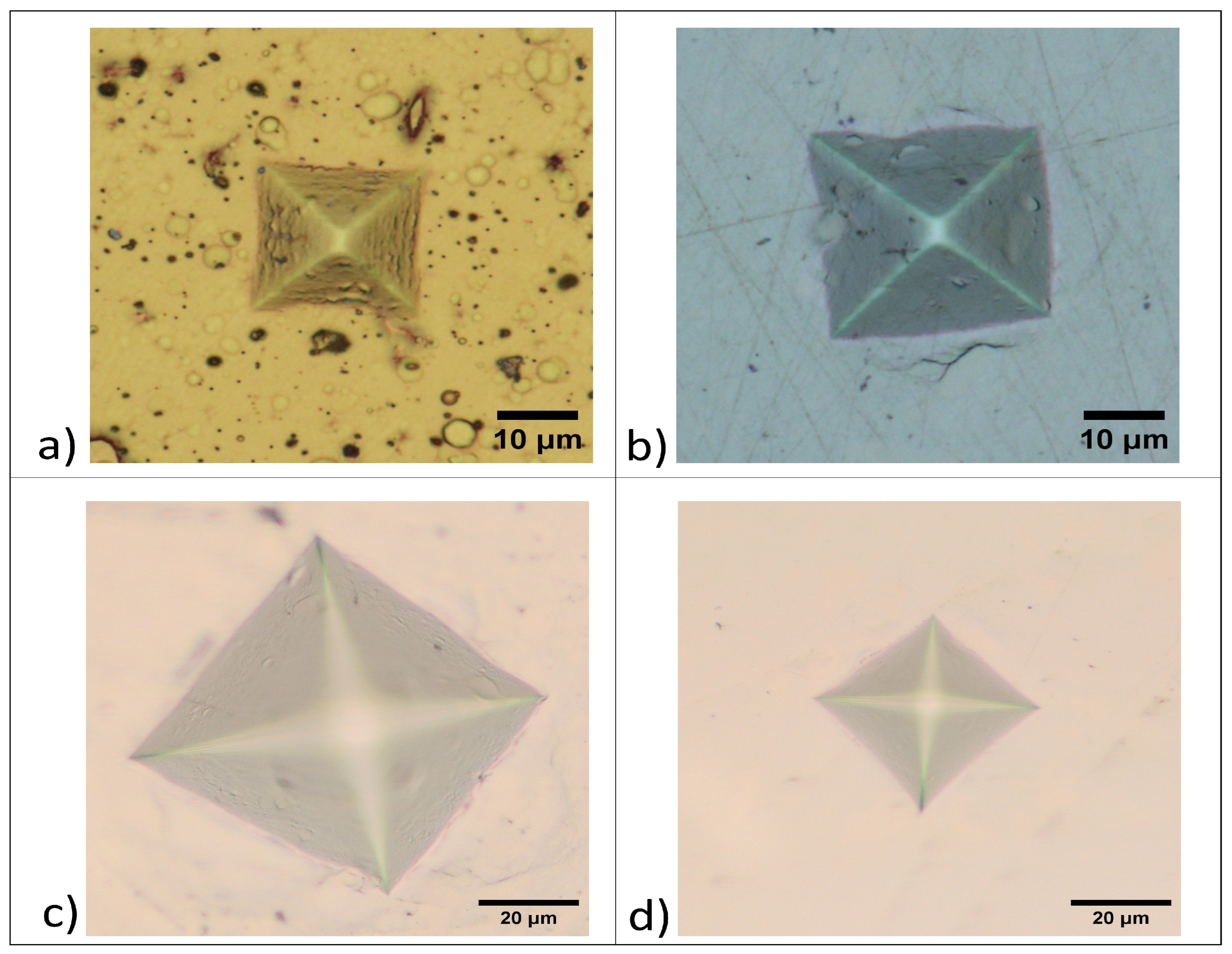
Table 2 shows the average hardness measured manually for each steel process. In total, 81 indentation images were used on D2 steel, including 42 with TiNbN coatings and 39 of steel with and without quenching and tempering heat treatment, as shown in Figure 2.
The indentations on the TiNbN-coated and tempered steel (Figure 2a,b) were performed using an Anton Paar RST3 scratch resistance tester, while the indentations on the steels with and without heat treatment (Figure 2c,d) were carried out using a NOVOTEST TB-MCV-1M microhardness tester. The range of load used for the first device was 1 N to 10 N and, for another tester, was 4.9 N to 9.8 N. The indentation images were captured at a magnification of 50× using an OLYMPUS UPRIGHT BX51FM trinocular metallographic microscope (Tokyo, Japan) equipped with a 10.2 Mpx SC100 camera.
In order to increase the size of the database for indentification purposes, data augmentation was performed by rotating the image every 5 degrees. The obtained images were reflected across the x and y axes (see Figure 2) and scaled up by increments of 10 until doubling the size of the original image, resulting in a total of 3000 images. Unlike the images used for localization, the bounding box of the indentation was utilized to locate the 4 corners, and the augmentation process developed for the indentation was repeated, resulting in a database of 12,000 images, in other words, 3000 images for each corner.
The method was developed using Python 3.7 language and the TensorFlow library. An Intel Xeon E5-2640 v4 computer (Santa Clara, CA, USA) with 12 cores at a base frequency of 2.2 GHz, 16 GB of RAM, and an NVidia Quadro M4000 graphics (Santa Clara, CA, USA) card with 8 GB GDDR5 was used.

2.2. Methods

2.2.1. Architectures of Neural Networks

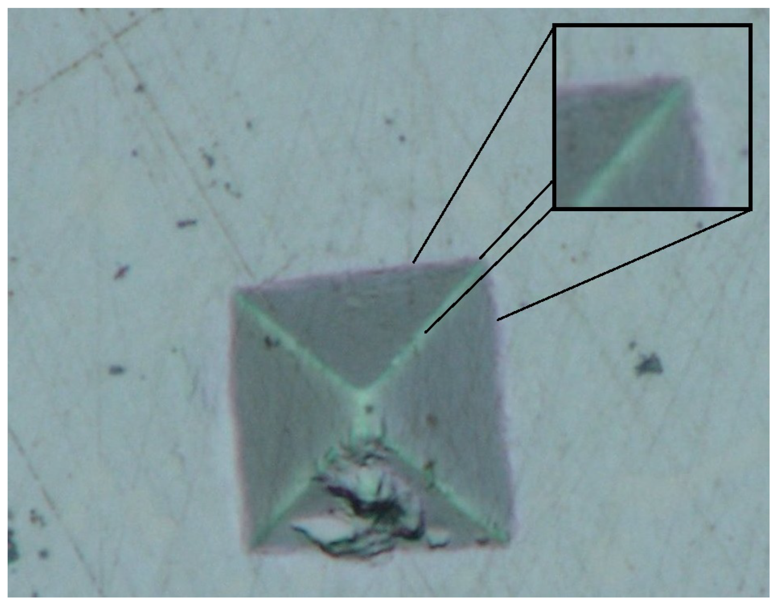
In the most recent works for fingerprint detection using neural networks, the entire fingerprint is used for training a neural network. In the case of Tanaka et al.’s method [8], the fingerprint must be positioned as a diamond shape to facilitate the detection of the corners. In contrast, this work aims to directly detect the corners, which enables time saving and improved accuracy. For this purpose, a training dataset was constructed consisting solely of corners of the fingerprints, as illustrated in Figure 3.
One state-of-the-art architecture used for object detection in images is YOLO v3, which offers the advantage of high computational efficiency [21]. This model divides the image into cells and calculates the probability of an object of interest being present in each cell [22]. Once an object is located, YOLO v3 uses five anchor boxes to define its boundaries [23]. It then compares the object existence probabilities to generate a new anchor box that best fits the object. Since indentations can have varying sizes, depending on image resolution and material hardness, YOLO v3 produces anchor boxes of different sizes. Therefore, YOLO v3 architecture is suitable for detecting indentations. YOLO is based on the Darknet-53 architecture, which utilizes 3 × 3 and 1 × 1 convolution filters and skip connections, and requires fewer billion floating-point operations (BFLOPs) compared to the ResNet architectures used by Tanaka [23], achieving the same classification accuracy percentage while being twice as fast, as shown in Table 3.

2.2.2. Implementation of the CNN (Convolutional Neural Network)

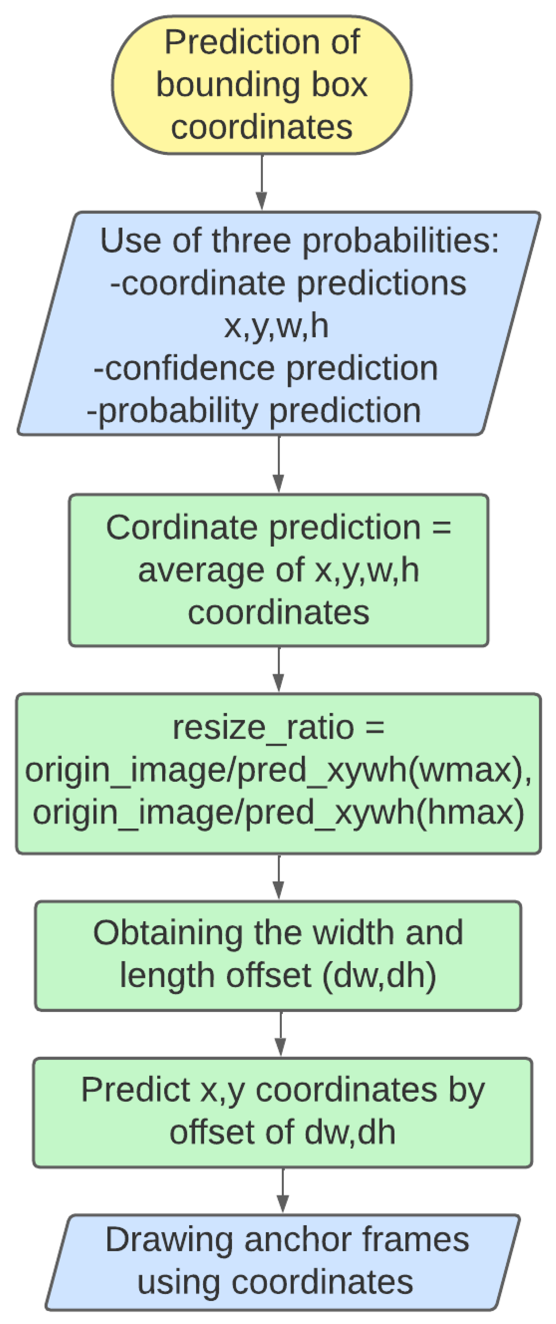
The following steps describe the flowchart shown in Figure 4:
  • Representative image of the indentation footprint: An image that exemplifies the indentation footprint used in the study is selected;
  • Image cropping and cleaning: The image is cropped to isolate the indentation footprint, and cleaning techniques are applied to remove noise and enhance its quality;
  • Data augmentation: A data augmentation technique is employed to increase the diversity of the training set. This involves applying random transformations, such as rotations, scaling, or contrast adjustments, to the existing images, thereby generating new training samples;
  • Dataset division: The dataset is divided into three subsets—an 80 % training set, a 15 % validation set, and a 5 % final test set;
  • YOLO adaptation for training: The YOLO neural network architecture is adapted and configured specifically for the detection of corners in indentation footprints. This involves addressing transfer learning, where the pre-trained weights of the neurons used for detecting the 80 classes in the COCO dataset are fine-tuned to detect a single class, which, in this case, is corners. This allows for more efficient training with a smaller training dataset;
  • Training set labeling using LabelImg: The LabelImg tool is used to manually label the corners of the indentation footprints in the training set. The coordinates of the corners are marked and annotated on each image;
  • Conversion from XML to YOLO format: The corner annotations in XML format are converted to a YOLO-compatible label format, which is typically a plain text file with a specific format;
  • Corner detection: A convolutional neural network (CNN) is employed to detect the corners in the processed indentation footprints. The CNN learns to identify relevant features that indicate the presence of a corner in an image, which are obtained through the convolutions that enrich the feature map;
  • Corner prediction: Once the corners are detected, predictions are made to determine the precise coordinates of the corners in the image, including object probabilities, confidence probabilities, and coordinate probabilities;
  • Euclidean distance scanning algorithm: An algorithm based on Euclidean distance scanning is applied to identify the corresponding corners that form the main diagonals of the indentation footprint. This allows for the measurement and calculation of the lengths of the main diagonals;
  • Drawing of the main diagonals: The main diagonals are drawn on the indentation footprint image to provide a clear and accurate visualization of the indentation geometry;
  • Conversion from pixels to micrometers: The pixel coordinates of the corners and the lengths of the diagonals are converted to micrometer units to obtain more precise and meaningful measurements, taking into account the scale at which the image was captured;
  • Input values into the Vickers hardness equation: The obtained values are used to calculate the Vickers hardness using the specific equation for this type of hardness test;
  • Determination of Vickers hardness value: Finally, the corresponding Vickers hardness value of the analyzed indentation footprint is determined, providing information about the material’s hardness.
For network tuning, a dataset of 3000 D2 steel indentation images was utilized, encompassing a variety of backgrounds, shades, and intensities. This diverse dataset enabled the trained network to independently identify corners, regardless of the background noise present in the image. The dataset was divided into training (80%), tuning (15%), and validation (5%). The dense Darknet network was fine-tuned using the training dataset, while the tuning set was used to monitor the accuracy of the CNN during training, employing the binary cross-entropy loss function (5) equation to encourage the neural network to produce outputs that closely matched the true labels during training, taking into account that the architecture also calculated three additional losses, namely, coordinate loss (4), confidence loss (2), and class loss (3).
i = 0 S 2 j = 0 B 1 i j o b j ( I O U i j p r e d I O U i j t r u e ) 2 λ n o o b j i = 0 S 2 j = 0 B 1 i j n o o b j ( I O U i j p r e d I O U i j t r u e ) 2
where S is the size of the feature map, B is the number of boxes per cell, 1 i j o b j is an indicator variable that is 1 if cell i in the feature map is assigned to object j and 0 otherwise, I O U i j p r e d is the intersection over union (IoU) between the prediction and ground truth for object j in cell i, I O U i j t r u e is the IoU between the prediction and ground truth for object j in cell i, 1 i j n o o b j is 1 if cell i is not assigned to any object and 0 otherwise, and λ n o o b j is a weighting coefficient for the confidence loss in cells that do not contain objects [24].
i = 0 S 2 j = 0 B 1 i j o b j c = 0 C ( I O U i j p r e d ( P i j p r e d ( c ) P i j t r u e ( c ) ) 2
where C is the number of classes, P i j p r e d ( c ) is the predicted probability that object j in cell i belongs to class c, and P i j t r u e ( c ) is the true probability that object j in cell i belongs to class c.
i = 0 S 2 j = 0 B 1 i j o b j ( ( x i j p r e d x i j t r u e ) 2 + ( y i j p r e d y i j t r u e ) 2 + ( w i j p r e d w i j t r u e ) 2 + ( h i j p r e d h i j t r u e ) 2 )
Taking into account that x i j p r e d and y i j p r e d are the predicted coordinates of the bounding box center for object j in cell i, w i j p r e d and h i j p r e d are the predicted dimensions of the bounding box for object j in cell i, and ( x , y , w , h ) i j t r u e are the true coordinates and dimensions of the bounding box for object j in cell i,
i = 0 S 2 j = 0 B 1 i j o b j ( l o g ( p ^ i j p r e d ) 1 i j o b j p i j t r u e + l o g ( 1 p ^ i j p r e d ) 1 i j o b j ( 1 p i j t r u e ) )
p ^ i j p r e d is the predicted probability that cell i in the feature map contains an object. In conclusion, the binary cross-entropy loss in YOLO measures the discrepancy between the object presence predictions and the ground truth labels, penalizing incorrect predictions using the algorithm of predicted probabilities and ground truth labels [24].
The labelImg tool was used for labeling the dataset. Although it remains a manual process to label each image by identifying the object of interest (corner), this tool assists in generating the bounding box coordinates and class label file, which are used for network training, as shown in Figure 5.
YOLO v3 was pre-trained for the detection of 80 classes of objects, not for the detection of points of interest within objects. Therefore, it was necessary to modify the outputs of the first layer of the architecture for the detection and localization of corner coordinates in the indentations. The initial layer of the CNN accepts images that are multiples of 32. In this case, a standard input size of 416 × 416 pixels was used, and all input images were resized to fit within a range of 160 × 172 to 676 × 642 pixels. The YOLO architecture is depicted in Figure 6. The fine-tuning parameters are presented in Table 4. It can be observed that the IoU threshold was set to 0.5, which was selected to cover the majority of objects of interest without sacrificing accuracy. A lower threshold leads to false detections, while a higher threshold results in more precise detections. However, in noisy images, such as those with NiTiNb coating, not all corners of the same indentation footprint are detected.
The initial learning rate of 0.0001 and the final learning rate of 0.000001 were variables; 182 and a smoother cosine function [26] were employed. This approach gradually reduced the learning rate from the initial value to 0 following a cosine function, as expressed in (6). This cosine function aided in preventing the loss function from ending up stuck in a local minimum. To obtain the coordinates and measurements of the diagonals, the output delivered by the CNN was configured as illustrated in Figure 7.
η i 1 2 1 + c o s i π T η
where η is the initial learning rate, T is the total number of batches, and i is the current batch.
To detect objects in an image, the following procedure was applied. Firstly, the image was divided into an S × S grid, and N possible bounding boxes and their probabilities were predicted for each grid cell. Subsequently, bounding boxes with a probability lower than a threshold of 0.6 were discarded. Next, a technique called non-max suppression was employed, which removed redundant bounding boxes that detected the same object and retained only the most accurate ones. Finally, the coordinates of the remaining bounding boxes were scaled to the original image size using a formula that depended on the input image size and the grid size [27]. The formula was as follows:
x r = S x p W
y r = S y p H
w r = S w p W
h r = S h p H
where x r , y r , w r , and h r are the actual coordinates of the center, width, and height of the bounding box in the original image; x p , y p , w p , and h p are the predicted coordinates of the center ( x , y ) , width, and height of the bounding box in the grid; S is the size of the grid; and W and H are the width and height of the original image.
The flowchart (see Figure 7) describes the specific steps used in YOLO for the prediction of bounding boxes. It provides a detailed understanding of how predictions are made and how the predicted coordinates are adjusted to the original image. These steps are essential for achieving accurate and efficient object detection in images using YOLO:
  • Use of three probabilities: During the prediction of bounding boxes, three distinct probabilities are used. The first is the coordinate prediction ( x , y , w , h ) , which represents the average of the predicted coordinates for each bounding box. The second is the confidence prediction, indicating how confident the model is that the object is present in the bounding box. The third is the probability prediction, assigning a probability to each object class within the bounding box;
  • Computation of the resizing factor: The resizing factor is calculated using the size of the original image and the maximum width ( w m a x ) and height ( h m a x ) values of the predicted bounding boxes. The resizing factor is obtained by dividing the size of the original image by the values w m a x and h m a x . This factor is used to adjust the predict coordinates to the scale of the original image;
  • Obtaining the width and height offset ( d w , d h ) : The width ( d w ) and height ( d h ) offsets of the bounding boxes are computed using the resizing factor. These offsets represent the difference between the actual size of the bounding boxes and the size predicted by the model;
  • Prediction of the x and y coordinates through the offset ( d w , d h ) : The predicted x and y coordinates are adjusted by considering the previously calculated width and height offsets. This is carried out by adding or subtracting the values of d w and d h to the predicted coordinates, depending on the position of the bounding box with respect to the original image;
  • Drawing the bounding boxes using the coordinates: Finally, the bounding boxes are drawn using the predicted coordinates and the resizing factor. These bounding boxes represent the delimited regions where the model has identified the presence of objects of interest.
The object probability in YOLO v3 is determined by generating bounding boxes that enclose potential objects in the image. Each bounding box has a score indicating the probability of containing an object, calculated based on the response of the detection layers. This score is combined with the corresponding class probability, representing the likelihood of belonging to a specific category, such as “corner” or “no corner”. The YOLO v3 approach enables efficient and accurate real-time object detection by performing the entire process in a single pass, achieving a balance between speed and precision in object classification.
Therefore, detecting the coordinate of the inner pixel of the bounding box represents the specific corner of the indentation footprint, which should be close to the center of the anchor box. Its pixel neighbors a pixel with a different tonality. Taking this into account, the center of the bounding box was found using
w i d t h ( x ) = ( x 2 x 1 ) 2 + x 1
h e i g h t ( y ) = ( y 2 y 1 ) 2 + y 1
Using Equations (11) and (12), the coordinate ( x , y ) corresponding to the center c of the bounding box where the corner of the indentation footprint found by the CNN was located was obtained. To find the exact point where the corner of the indentation footprint was located, the pixels within the bounding box were first binarized using the skimage.filters library to determine the optimal threshold. Then, the contour was obtained using the OpenCV findContours library. After this step, the approxPolyDP function was used to obtain the triangular geometry formed at the corner of the indentation footprint. This function approximates a contour shape with a reduced number of vertices. Finally, to locate the precise point where the triangle corner was formed, the pixels along the boundary between the two thresholded regions, one corresponding to the background and the other to the indented region, were traced, as shown in Figure 8. The pixel that was farthest from the boundary and aligned with the height of the triangle was considered as the pixel corresponding to the position of the corner.
Once the four corners of the indentation footprint (V) had been identified, it was necessary to arrange them within the footprint in order to find the main diagonals. To achieve this, the first located corner a was selected, and the corner d located farthest from a was identified using the Euclidean distance, while the remaining two corners corresponded to points b and c, as shown in Figure 9. The vector of data containing the coordinates of the pixels corresponding to each corner of the indentation footprint was traversed.
Using the following notation for the corner coordinates: a = ( x 1 , y 1 ) , b = ( x 2 , y 2 ) , c = ( x 3 , y 3 ) , d = ( x 4 , y 4 ) , the main diagonals of V were calculated.
One of those coordinates within the rectangles was randomly chosen as a reference point, and each rectangle center was denoted as a = ( x 1 , y 1 ) , b = ( x 2 , y 2 ) , c = ( x 3 , y 3 ) , d = ( x 4 , y 4 ) , taking into account that they would be close to the center of the bounding box. Next, the Euclidean distance between them was calculated to have a parameter for comparison and to determine which corner was correct for forming the diagonal. The pair of corners with the greatest distance was the correct pair, while the remaining corners formed the missing pair. The distances between points were obtained using Equations (13) and (14):
d 3 = a d x + a d y
d 3 = b c x + b c y
Finally, the values of the two diagonals, d 1 and d 2 , were averaged to obtain the Vickers hardness value using Equation (1).

3. Results

3.1. Identifier Using Transfer Learning

In this section, the results obtained using a classifier are presented. After different training sessions of the CNN, it was determined that the maximum accuracy percentage was achieved at 100 epochs. Therefore, the network was retrained only up to 100 epochs to prevent overfitting (Figure 10a). A high accuracy rate of 92% was achieved, indicating the effectiveness of the proposed classifier. Importantly, an ascending behavior in the CNN’s accuracy was observed when identifying a new class, specifically, the corners. The CNN successfully located and precisely delineated these corners in the corresponding frames (Figure 10a).
Furthermore, during the training process, it was observed how the binary cross-entropy (loss function) significantly penalized values that were considered reliable but were not. This function assigned a high value to those close to 1 and a very small value to values close to 0. A value of 1 or close to 1 indicates high confidence in the precise delineation of the frame, i.e., its similarity to the ground truth.
These results demonstrate the algorithm’s ability to efficiently converge towards loss minimization in a short period, as observed in Figure 10b. The combination of the high accuracy rate and the network’s capability to accurately locate and delineate corners makes this classifier a promising tool for object detection and localization in images. Detailed experiments and their corresponding results are presented in the following sections.
The obtained data were in line with what is shown in Figure 11, where Lu Tan et al. [28] compared the YOLO v3 model with RetinaNet and SSD (Single Shot Multi-Box Detector) networks using different metrics such as F1 score, mAP (Mean Average Precision), Precision, and Recall. YOLO v3 demonstrated superior results compared to the other two architectures.

3.2. Corner Identification on Final Test Images

In Figure 12, the detection of corners obtained with the proposed model can be observed. In Figure 12a,b, the algorithm identified the location of the corners when they did not exhibit pores or surface scratches and had the same orientation. On the other hand, in Figure 12c,d, pores were observed in the corners, possibly due to coating delamination. This can pose a challenge in corner detection; however, the proposed method successfully identified them.

3.3. Corner Identification on Other Images

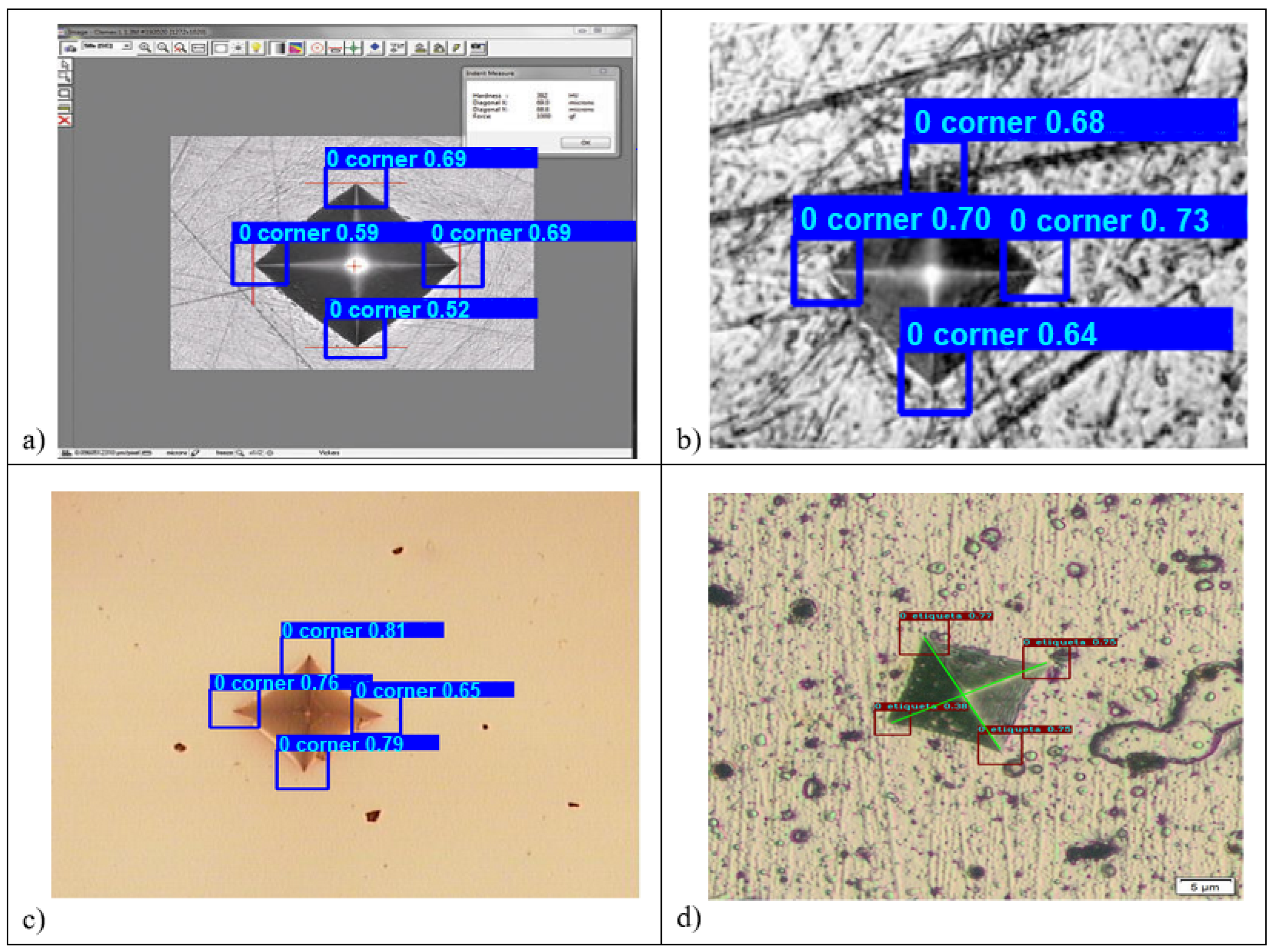
In order to verify the robustness of the developed method, two images available on the internet and two images from the experiments with indentations and different backgrounds were selected (see Figure 13). As can be seen, the method correctly identified the corners of the indentation mark in each image. This additional evidence supports the capability of the proposed model to accurately detect and locate corners under various conditions and environments.
To assess the robustness of the developed method, four images were selected, representing different scenarios: two images obtained from the internet and two images obtained experimentally. These images featured indentations with diverse backgrounds, as shown in Figure 13. The developed method demonstrated its capability to accurately identify the corners of the indentation marks in each of these images. This additional support confirms the precision and effectiveness of the proposed model for the detection and localization of corners under different conditions and environments.

3.4. Drawing of Main Diagonals

The indentation marks presented in Figure 14 show two positions, one located with the same orientation as used by Tanaka [8] (see Figure 14a), and the other corresponds to a footprint with a different orientation (see Figure 14b), demonstrating the correct identification of corners and diagonals, independent of the orientation of the indentation mark.

3.5. Comparison between the Tanaka Method and the One Developed

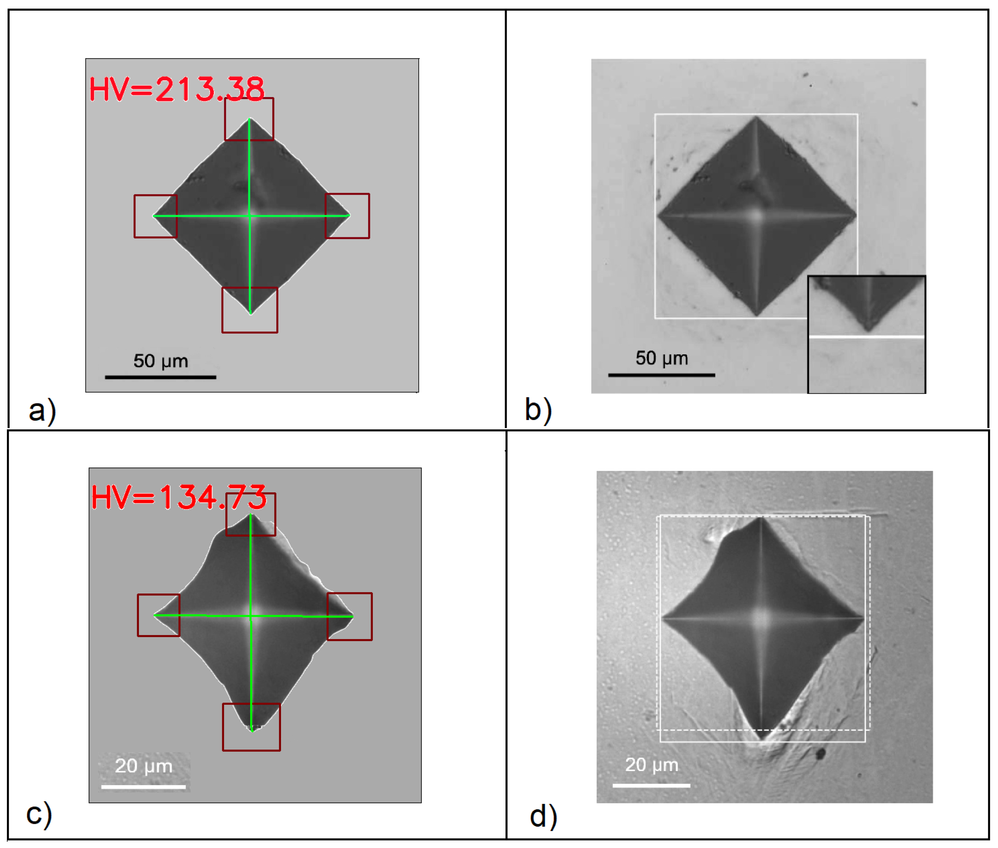
In this section, two images from Tanaka’s article [8] are included, which contain the measurement scale from pixels to micrometers. This scale was obtained using imageJ. The images were processed to remove the background of the indentation trace because the squares enclosing Tanaka’s indentation trace in Figure 15b,d caused errors in corner identification by YOLO. Subsequently, both images were inputted into the CNN, along with the scale parameters and the applied load for each indentation trace, in order to determine the Vickers hardness value. These results were collected in Table 5.

3.6. Comparison between the Manual Measurement and the One Developed

The developed method was applied to an indentation mark made on tempering D2 steel (Figure 16a) with a hardness value of H V = 530.17 , and on D2 steel with TiNbN coating (Figure 16c) under a 10 N load, measured manually. By inputting the image shown in Figure 16a), the values of both diagonals were obtained, which corresponded to 58.95 ( μ m) and 58.12 ( μ m), respectively (see Figure 16b). After determining the values of the diagonals, they were averaged, and Equation (1) was used to calculate the hardness value.
D = 58.95 μ m + 58.12 μ m 2 = 58.54 μ m
H V = 0.1891 × 10 N ( 0.05854 mm ) 2 = 551.81 N mm 2
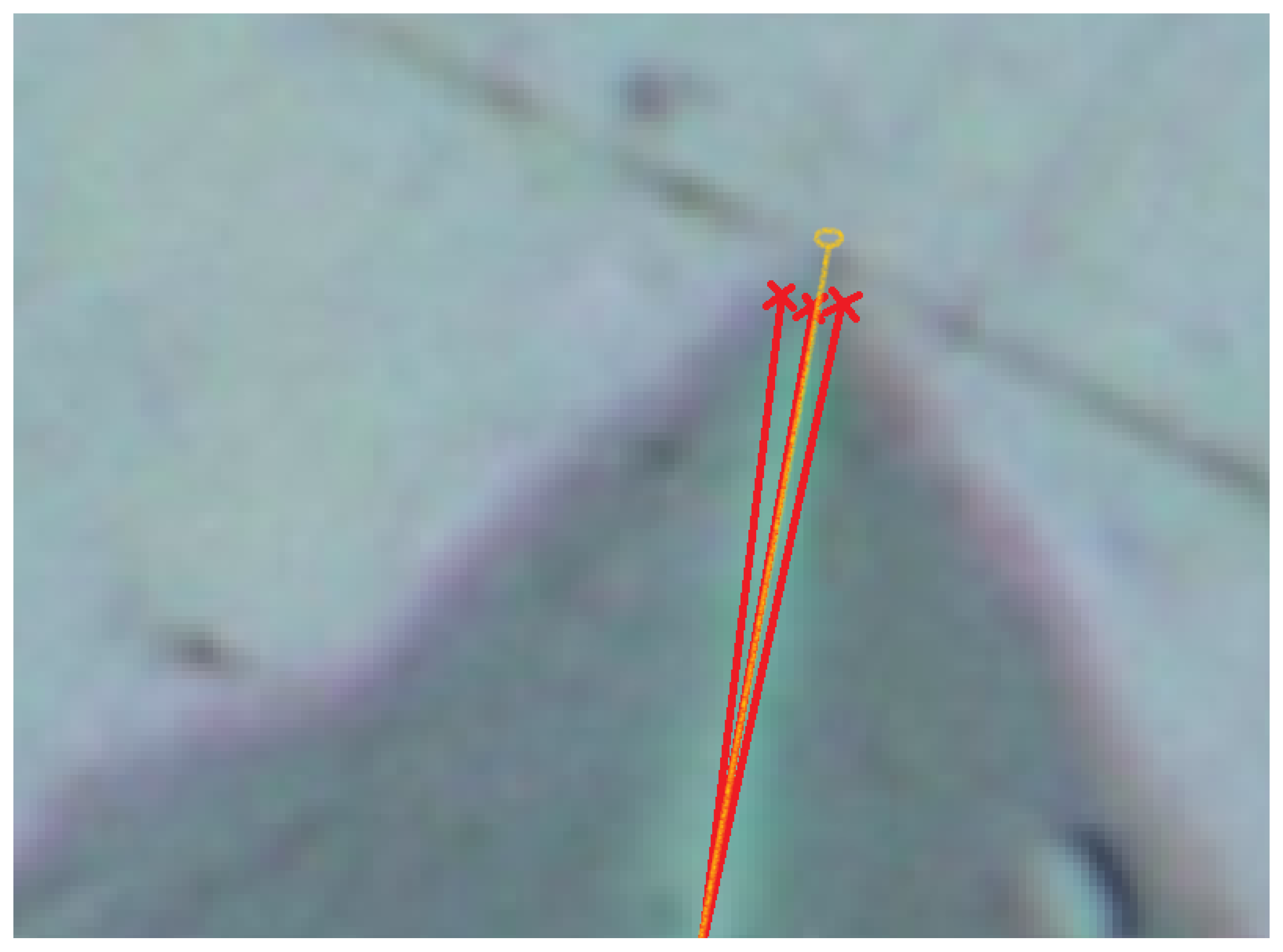
The hardness value obtained using the proposed method for tempered D2 steel were 551.81 H V , while, for the coated steel, it was 1067.42 H V . This resulted in an error percentage of 4.08 % for tempered steel and 5.43 % for coated steel. In the Table 5, the values of manual hardness and those obtained by the proposed method for 36 randomly acquired images are not displayed. It is noteworthy that the error percentage between the manual values and those obtained by the algorithm ranges from 0.17 % to 5.98 % . These results are comparable to those obtained by other authors, ranging from 0.32 % to 4.5 % for Polanco [11], and from 1 % to 11.56 % , depending on the material type, for Tanaka [8]. To determine if the error produced by the model was higher than that produced by the experts, a close-up analysis was performed on the corners detected by the model and those detected by the experts. It was found that the error produced by the experts was greater and not reproducible compared to the error generated by the method in corner localization, as shown in Figure 17.
The red marks represent the markings that may be made by researchers, as these are subjective to each individual, based on where they believe the corner of the indentation mark is located. Furthermore, it is unlikely that the researcher will mark the exact same corner on the same pixel of the same image, making the manual method non-reproducible. In contrast, the yellow markings depict the markings generated by the developed method, which are reproducible.

4. Conclusions

This article presents a novel method for calculating Vickers hardness using corner detection based on convolutional neural networks, achieving an accuracy of 92 % . The method is effective across three different types of images, eliminating the need for model adjustments. This enables the measurement of diagonals, regardless of the position of indentation imprints in the image, and is applicable to various materials, including steel under different conditions.
Additionally, the hardness value is determined by measuring the diagonals, resulting in a relative error of 0.17 % to 5.98 % for the 36 images used. A comparison with manual markings performed by human experts demonstrates that the proposed method surpasses subjective manual approaches, providing reproducible results. These findings establish the reliability and applicability of the proposed method for analyzing indentations in diverse conditions and environments.

Author Contributions

Conceptualization and supervision, M.G.F. and J.F.P.; methodology, validation, and formal analysis, M.G.F., J.C.B.D., J.F.P. and C.L.M.; software development, M.G.F. and J.C.B.D.; image acquisition and data curation, C.L.M., J.F.P. and C.O.-P.; writing and writing—review, editing, and visualization, all authors, project administration and funding acquisition, J.F.P. All authors have read and agreed to the published version of the manuscript.

Funding

The APC was funded by Universidad de Ibagué (19-506-INT) and Universidad Señor de Sipán.

Institutional Review Board Statement

Not applicable.

Informed Consent Statement

Not applicable.

Data Availability Statement

Not applicable.

Conflicts of Interest

The authors declare no conflict of interest.

References

  1. Castillo Gutiérrez, D.E.; Angarita Moncaleano, I.I.; Rodríguez Baracaldo, R. Microstructural and mechanical characterization of dual phase steels (ferrite-martensite), obtained by thermomechanical processes. Ingeniare Rev. Chil. Ing. 2018, 26, 430–439. [Google Scholar] [CrossRef]
  2. Arenas, W.; Martínez, O. Roughness and hardness optimization of 12L-14 steel using the response surface methodology. Ing. Ind. 2019, 37, 125–151. [Google Scholar] [CrossRef]
  3. Ageev, E.; Khardikov, S. Processing of Graphic Information in the Study of the Microhardness ofthe Sintered Sample of Chromium-containing Waste. In Proceedings of the CEUR Workshop, Pescaia, Italy, 16–19 June 2019; pp. 252–255. [Google Scholar] [CrossRef]
  4. Koch, M.; Ebersbach, U. Experimental study of chromium PVD coatings on brass substrates for the watch industry. Surf. Eng. 1997, 13, 157–164. [Google Scholar] [CrossRef]
  5. ASTM E384-99; Standard Test Method for Microindentation Hardness of Materials. ASTM International: West Conshohocken, PA, USA, 2017; pp. 1–40. [CrossRef]
  6. ASTM E92-17; Standard Test Methods for Vickers Hardness and Knoop Hardness of Metallic Materials. ASTM International: West Conshohocken, PA, USA, 2017; pp. 1–27. [CrossRef]
  7. Buehler. Pruebas de Dureza Vickers. Available online: https://www.buehler.com/es/blog/pruebas-de-dureza-vickers/ (accessed on 23 June 2023).
  8. Tanaka, Y.; Seino, Y.; Hattori, K. Automated Vickers hardness measurement using convolutional neural networks. Int. J. Adv. Manuf. Technol. 2020, 109, 1345–1355. [Google Scholar] [CrossRef]
  9. Dominguez-Nicolas, S.M.; Wiederhold, P. Indentation image analysis for vickers hardness testing. In Proceedings of the 2018 15th International Conference on Electrical Engineering, Computing Science and Automatic Control (CCE 2018), Mexico City, Mexico, 5–7 September 2018; pp. 1–6. [Google Scholar] [CrossRef]
  10. Sugimoto, T.; Kawaguchi, T. Development of an automatic Vickers hardness testing system using image processing technology. IEEE Trans. Ind. Electron. 1997, 44, 696–702. [Google Scholar] [CrossRef]
  11. Polanco, J.D.; Jacanamejoy-Jamioy, C.; Mambuscay, C.L.; Piamba, J.F.; Forero, M.G. Automatic Method for Vickers Hardness Estimation by Image Processing. J. Imaging 2023, 9, 8. [Google Scholar] [CrossRef] [PubMed]
  12. Abiodun, O.I.; Jantan, A.; Omolara, A.E.; Dada, K.V.; Mohamed, N.A.; Arshad, H. State-of-the-art in artificial neural network applications: A survey. Heliyon 2018, 4, e00938. [Google Scholar] [CrossRef] [PubMed] [Green Version]
  13. Satat, G.; Tancik, M.; Gupta, O.; Heshmat, B.; Raskar, R. Object classification through scattering media with deep learning on time resolved measurement. Opt. Express 2017, 25, 17466–17479. [Google Scholar] [CrossRef] [PubMed] [Green Version]
  14. Salazar Guerrero, J.E. Implementación de un Prototipo de Sistema Autónomo de Visión Artificial para la Detección de Objetos en Vídeo Utilizando Técnicas de Aprendizaje Profundo. 2019. Available online: http://repositorio.espe.edu.ec/handle/21000/20995 (accessed on 23 June 2023).
  15. Weiss, K.; Khoshgoftaar, T.M.; Wang, D.D. A survey of transfer learning. J. Big Data 2016, 3, 9. [Google Scholar] [CrossRef] [Green Version]
  16. Hussain, M.; Bird, J.J.; Faria, D.R. A Study on CNN Transfer Learning for Image Classification; Springer: Berlin/Heidelberg, Germany, 2019; Volume 840, pp. 191–202. [Google Scholar] [CrossRef]
  17. Jalilian, E.; Uhl, A. Deep Learning Based Automated Vickers Hardness Measurement. In Proceedings of the Computer Analysis of Images and Patterns, Virtual Event, 28–30 September 2021; Tsapatsoulis, N., Panayides, A., Theocharides, T., Lanitis, A., Pattichis, C., Vento, M., Eds.; Springer International Publishing: Cham, Switzerland, 2021; pp. 3–13. [Google Scholar] [CrossRef]
  18. Li, Z.; Yin, F. Automated measurement of Vickers hardness using image segmentation with neural networks. Measurement 2021, 186, 110200. [Google Scholar] [CrossRef]
  19. Cheng, W.S.; Chen, G.Y.; Shih, X.Y.; Elsisi, M.; Tsai, M.H.; Dai, H.J. Vickers Hardness Value Test via Multi-Task Learning Convolutional Neural Networks and Image Augmentation. Appl. Sci. 2022, 12, 10820. [Google Scholar] [CrossRef]
  20. Gonzalez-Carmona, J.M.; Mambuscay, C.L.; Ortega-Portilla, C.; Hurtado-Macias, A.; Piamba, J.F. TiNbN Hard Coating Deposited at Varied Substrate Temperature by Cathodic Arc: Tribological Performance under Simulated Cutting Conditions. Materials 2023, 16, 4531. [Google Scholar] [CrossRef] [PubMed]
  21. Redmon, J.; Divvala, S.K.; Girshick, R.B.; Farhadi, A. You Only Look Once: Unified, Real-Time Object Detection. In Proceedings of the 2016 IEEE Conference on Computer Vision and Pattern Recognition (CVPR), Las Vegas, NV, USA, 27–30 June 2016. [Google Scholar]
  22. Redmon, J.; Farhadi, A. YOLOv3: An Incremental Improvement. arXiv 2018, arXiv:1804.02767. [Google Scholar]
  23. He, K.; Zhang, X.; Ren, S.; Sun, J. Deep Residual Learning for Image Recognition. arXiv 2015, arXiv:1512.03385. [Google Scholar]
  24. Zhao, L.; Li, S. Object Detection Algorithm Based on Improved YOLOv3. Electronics 2020, 9, 537. [Google Scholar] [CrossRef] [Green Version]
  25. Ammar, A.; Koubaa, A.; Ahmed, M.; Saad, A.; Benjdira, B. Vehicle Detection from Aerial Images Using Deep Learning: A Comparative Study. Electronics 2021, 10, 820. [Google Scholar] [CrossRef]
  26. Otomo, H.; Zhang, R.; Chen, H. Improved phase-field-based lattice Boltzmann models with a filtered collision operator. Int. J. Mod. Phys. 2018, 30, 1941009. [Google Scholar] [CrossRef] [Green Version]
  27. Gai, W.; Liu, Y.; Zhang, J.; Jing, G. An improved Tiny YOLOv3 for real-time object detection. Syst. Sci. Control. Eng. 2021, 9, 314–321. [Google Scholar] [CrossRef]
  28. Tan, L.; Huangfu, T.; Wu, L.; Chen, W. Comparison of RetinaNet, SSD, and YOLO v3 for real-time pill identification. BMC Med. Inform. Decis. Mak. 2021, 21, 324. [Google Scholar] [CrossRef] [PubMed]
  29. ZwickRoell. Durómetro ZHVμ. Available online: https://www.zwickroell.com/es/productos/equipos-de-ensayos-de-dureza/durometros-vickers/zhvm/ (accessed on 15 May 2022).
  30. Lloyd Instruments. Microhardness Testing—Minimizing Common Problems. AZoM. Available online: https://www.azom.com/article.aspx?ArticleID=10807 (accessed on 15 May 2022).
  31. Ebatco. Microindentation. Available online: https://www.ebatco.com/laboratory-services/mechanical/microindentation/ (accessed on 10 May 2022).
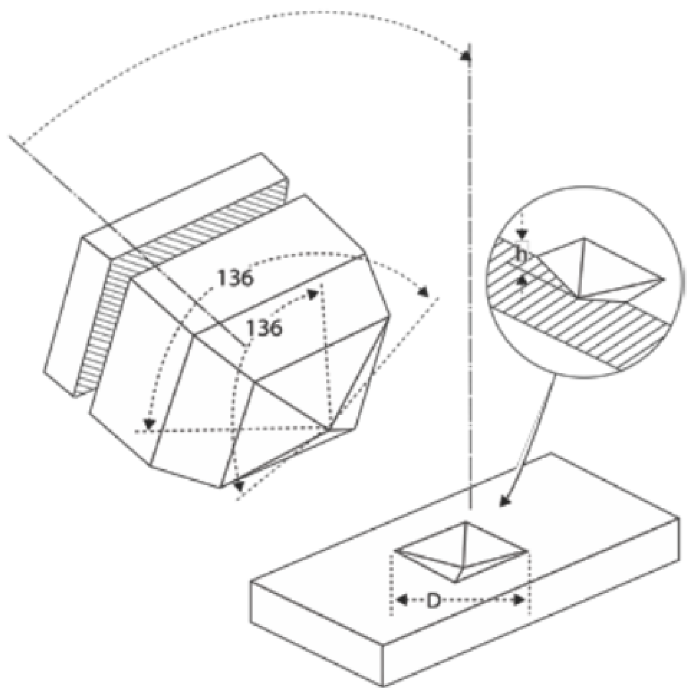
Figure 1. Diagram of the Vickers indenter and impression shape [7].
Metals 13 01391 g001
Figure 2. Category of images used for the construction of the database: (a) TiNbN coating, (b) tempered D2 steel, (c) D2 steel without heat treatment, and (d) quenched D2 steel.
Metals 13 01391 g002
Figure 3. Corner of indentation imprints.
Metals 13 01391 g003
Figure 4. Diagram of the prediction process.
Metals 13 01391 g004
Figure 5. Process employed for sampling and labeling the corners of an indentation imprint.
Metals 13 01391 g005
Figure 6. YOLO v3 network structure with layer inputs and outputs [25].
Metals 13 01391 g006
Figure 7. Flowchart for obtaining coordinates of the corners of the indentation imprint.
Metals 13 01391 g007
Figure 8. Image thresholding.
Metals 13 01391 g008
Figure 9. Measurement of corners in the indentation imprint.
Metals 13 01391 g009
Figure 10. Training for 100 epochs: (a) Accuracy achieved during training, (b) Convergence of the error function.
Metals 13 01391 g010
Figure 11. Comparison of CNNs in accuracy metrics (mAP, F1, Recall) over 100 training epochs [28].
Metals 13 01391 g011
Figure 12. Corner detection results: (a,b) D2 steels with similar orientations and (c,d) TiNbN coatings with different orientations and noise in the corners.
Metals 13 01391 g012
Figure 13. Corner detection results in different materials: (a) Computer-generated tools (noise) with the indentation background [29], (b) Cracks in the indentation with color variations (adapted from [30]), (c) Indentation with non-rectangular geometry, (d) Indentation with porous and scratched background.
Metals 13 01391 g013
Figure 14. Detection and measurement results of diagonals in different materials: (a) D2 steel indentation, (b) Indentation with a different background [31].
Metals 13 01391 g014
Figure 15. Comparison between the developed method and Tanaka’s method: (a) indentation footprint of 200 HV (Tanaka does not mention the material of this sample) and (c) indentation footprint of titanium of 130 HV; figures (b,d) are those of Tanaka.
Metals 13 01391 g015
Figure 16. Detection and measurement of the principal diagonals in the indentation marks: (a,c) Original image, (b,d) Original image with detected corners and marked diagonals.
Metals 13 01391 g016
Figure 17. Comparison between manual marking by human personnel (red line) and marking generated by the developed method (yellow line).
Metals 13 01391 g017
Table 1. Chemical composition and coating thickness [20].
Ts (°C)Ti (at%)Nb (at%)N (at%)Thickness ( μ m)
20057.86 ± 7.280.21 ± 0.0141.93 ± 7.274.68 ± 0.03
40051.06 ± 0.570.18 ± 0.0248.76 ± 0.586.80 ± 0.12
60044.72 ± 3.090.15 ± 0.0255.12 ± 3.085.93 ± 0.04
Table 2. Average Vickers hardness.
Load (N)Steel (HV)Quenched (HV)Tempered (HV)TiNbN-200 (HV)TiNbN-400 (HV)TiNbN-600 (HV)
1 576.25 ± 87.192106.27 ± 82.411935.61 ± 111.471701.23 ± 107.64
2 650.93 ± 39.381581.30 ± 41.661537.44 ± 135.491435.31 ± 12.20
3 596.64 ± 14.371476.44 ± 214.361290.03 ± 3.831331.98 ± 70.11
4.9157.44 ± 2.97542.86 ± 10.93
5 578.89 ± 24.171303.58 ± 173.801044.25 ± 41.491024.40 ± 21.92
9.8243.78 ± 5.04796.16 ± 9.61639.54 ± 17.10
10 533.82 ± 3.691009.21 ± 14.53846.24 ± 49.16844.35 ± 49.02
Table 3. Performance comparison of architectures employed for indentation imprint detection using the COCO database [21].
ArchitectureBFLOP (%)AccuracyTime(ms)
Darknet-197.2991.85.84
ResNet-10119.793.718.86
ResNet-15229.493.827.02
Darknet-5318.793.812.82
Table 4. Fine-tuning parameters of the model.
ParametersValue
Data transferTrue
COCO datasetFalse
Training epochs100
Batch4
lr1 × 10 3 a 1 × 10 6
Neurons2535
Threshold IoU0.5
Table 5. Diagonal length and Vickers hardness using the Tanaka [8] and YOLO methods.
Diagonal Length ( μ m)Vickers Hardness (HV)
Load (N)ManualTanakaPurpose MethodeManualTanakaPurpose Methode
9.80793.793.693.3211.4211.6213.38
1.96154.654.352.4124.8126.2134.7
Disclaimer/Publisher’s Note: The statements, opinions and data contained in all publications are solely those of the individual author(s) and contributor(s) and not of MDPI and/or the editor(s). MDPI and/or the editor(s) disclaim responsibility for any injury to people or property resulting from any ideas, methods, instructions or products referred to in the content.