Abstract
The aim of this work is to describe a reliable methodology for determining parameters of a material model suitable for implementation in a welding simulation using the finite element method (FEM). The adopted methodology employs a multi-scale approach integrating a microstructure evolution model, a representative volume element (RVE) calibrated through experimental methods, including a thermal–mechanical simulator, and electron backscatter diffraction (EBSD) experiments. The result is a complete material model, which covers thermal, mechanical and metallurgical material models for SAF2507 (EN 1.4410), that shows promising results and was successfully implemented in finite element (FE) code. A direct comparison of experimental and calculated results shows a deviation of up to 12% for the phase fraction of austenite and 25% for the mean grain diameter of ferrite.
1. Introduction
The super-duplex EN. 14410, more commonly known as SAF2507, is widely used and applied in a variety of different industries, including chemical industries, pulp and paper industries and many more [1]. This high-alloyed steel is characterized by its good stress corrosion cracking properties, which are due to its 50:50 distribution of ferrite and austenite [2]. A slight deviation from this distribution, however, can severely diminish its properties [3], and thus well-designed processes are required when welding SAF2507. In the past, many experiments needed to be conducted to determine the best welding parameters, but due to the increasing availability of computational power, welding simulations are becoming a more common tool for the modern welding engineer.
Currently, finite element codes are available for simulating welding processes at various levels of complexity. The state of the art of such simulations is the prediction of the thermal cycles occurring at different positions around the weld; however, the induced phase transformations and the mechanical response, including residual stresses, can also be predicted [4,5].
Process engineers responsible for optimizing welding processes to achieve desired microstructures or to control local mechanical properties and residual stresses require simulations with the full complexity currently possible [6].
A prerequisite for such simulations of the welding process is the availability of a reliable material model that can predict all relevant phenomena with sufficient accuracy and reliability [6]. A particular challenge is to reliably predict the microstructure evolution, starting with the initial microstructure and ending with the microstructure that remains after post-weld cooling. The microstructure has a significant influence on the mechanical properties and is therefore essential for the reliable prediction of stresses and strains throughout the process.
The microstructural characteristics of super-duplex stainless steels (SDSSs) were covered in detail by S. Sharafi during his PhD [7] and the accompanying publications. The plastic deformation behavior of duplex stainless steels (DSSs) was investigated by M. Nyström [8]. However, to the best of our knowledge, there is no complete and reliable material model in the literature today that allows for a coupled prediction of the evolution of temperature, microstructure, mechanical properties and stresses and strains throughout the whole process of welding SAF2507.
The unique demands of welding processes necessitate a model that accurately represents microstructural changes and corresponding mechanical behavior across a broad temperature spectrum, from room temperature to the melting point, accommodating fast heating and cooling rates.
This work presents a material model tailored to predict the macroscopic deformations and stresses as well as the microstructure evolution during a plasma arc welding process of thin metal sheets, but it could easily be adapted to other welding procedures once implemented in a finite element code.
The present paper is divided into three parts. The first part will be devoted to an introduction to DSS with a focus on welding SAF2507 and the corresponding challenges. In the second part, the methodology, the experimental and numerical methods used to determine the presented model parameters are described. In the final part, the results of the multi-scale approach as well as the calculated single-phase flow curves will be discussed and analyzed.
2. Materials and Methods
This section provides an overview of DSS and the applied experimental and numerical methods, while the results are presented in Section 3.
2.1. Duplex Stainless Steels
The original definition of DSS was a two-phase ferritic–austenitic microstructure, with both components having more than 13 . In practical use, however, most DSSs have a rather even volumetric phase distribution of ferrite and austenite of around 50:50. Compared to austenitic stainless steels, DSSs have several advantages, such as higher mechanical strength, better resistance to stress corrosion cracking and a lower price due to a lower nickel content [9]. In the temperature range of 50 to 250 °C, the resistance to stress corrosion cracking and to pitting is better than that of austenitic stainless steels, which have a similar price [1]. These facts coupled with the fine grain size, which greatly increases the yield strength, give the DSSs certain advantages over austenitic stainless steels [9]. DSSs are classified into four different groups according to their pitting resistance equivalent (PRE) [10,11]:
- Lean duplex with a PRE of less than 35—a common grade would be S32304 (EN 1.4362), with a PRE only slightly higher than the comparable austenitic counterpart 316L (EN 1.4401)
- “Standard” duplex with a PRE of 35 to 40—an example of that grade would be S32205 (EN 1.4462).
- “Super” duplex with a PRE between 40 and 45—an example would be SAF2507 (S32750 or EN 1.4410), which is the main focus of this publication, with a PRE of 42.
- “Hyper” duplex with a PRE over 45—an example would be UNS S33207, with a PRE of over 50.
The chemical composition of the examined SAF2507 is listed in Table 1.

Table 1.
Chemical composition of SAF2507 as stated by the material certificate provided by the manufacturer.
2.2. Microstructure of Duplex Stainless Steels
Most DSSs solidify mostly as ferrite [12]. At higher temperatures, typically between 1050 °C and 1350 °C, only ferrite () and austenite () are stable, with the fraction of ferrite increasing with increasing temperature as shown in Figure 1a. It needs to be mentioned that CALPHAD-based [13] phase diagrams only provide information for the thermodynamic equilibrium. As such, they are of little importance for welding, but they still give a good overview of possible microstructures that could be chemically possible. In welding, the two-phase weld microstructure depends primarily on the chemical composition. The Schaeffler phase diagram [14] (see Figure 1b) was originally used for the evaluation of the weld microstructure resulting from rapid cooling after welding [6]. Nowadays, FE calculations can be used to more accurately calculate the temperature field during welding. Considering the formulas given for the chromium equivalent and the nickel equivalent , one can see the effects of the alloying elements on the resulting microstructure after welding [7]. For example, nitrogen N is an austenite-stabilizing alloying element that was added to help the formation of austenite and thus improve the corrosion properties [9,15].
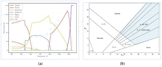
Figure 1.
The specific phase diagram of SAF2507 and the general Schaeffler diagram illustrating the relevant phases in duplex stainless steels and their microstructure. (a) Equilibrium phase diagram of SAF2507 predicted with JMatPro 12 with the chemical composition given in Table 1. (b) Schaeffler diagram as presented by [14], with a highlighted section to represent the duplex region and a point to illustrate the position of SAF2507.
The microstructure evolution model proposed by Hemmer et al. [16] takes into account the higher mobility of nitrogen and is based upon the published data of the nitrogen solubility in delta ferrite and austenite.
In the case of welding, not every phase or precipitation needs to be considered, since several phases, such as, for example, the phase, need more time to form than is available during welding [17,18].
The typical processing steps during the production of DSS plates are hot rolling and cold rolling followed by a final annealing step. This results in a microstructure with elongated grains that are almost pancake-like, as shown in Figure 2.
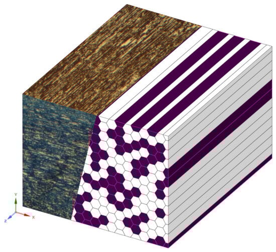
Figure 2.
Beraha II etchings of the SAF2507 base material shown together with a schematic of the used representative volume element (RVE) to illustrate the duplex microstructure. The size of the hexagons used in the actual calculations were on the same scale as the experimentally measured area-weighted diameter of the grains; see Section 2.3 for more details.
General overviews of DSSs and their respective phases, including relevant precipitates, can be found in [10,11,19,20], and an overview of the historical progression of the and can be found in [7].
2.3. Experimental Methods
For a representative experimental simulation of the welding conditions, namely the high heating and cooling rates as well as the high temperatures, a series of tests with a Gleeble® DSI 3800 thermal–mechanical simulator was conducted.
The thermal–mechanical simulator was used to prescribe exact heating–cooling cycles on the samples, to measure two-phase flow curves and to create the experimental specimens used for the characterization of the final microstructure at room temperature.
The thermal–mechanical experiments are categorized into two types: (a) stationary experiments and (b) non-stationary experiments. In the case of (a), the phase fractions of ferrite and austenite are close to thermodynamic equilibrium while, in the case of (b), the transformation from the ferrite to austenite is still ongoing when the mechanical load is applied. A test series for each type of experiments was carried out. All samples were heated to a target temperature of 1250 °C with a heating rate of 423 K/s and a holding time at the target temperature to establish a consistent microstructural initial state for all experiments. Subsequently, a tensile test with a defined strain rate was performed at a specified temperature below 1250 °C. Tensile tests were performed up to a maximum strain of 0.03 mm/mm to limit the occurrence of recrystallization, which could influence the flow curves used for fitting the material model and the microstructural investigations after quenching to room temperature. Further details on the test parameters are given in Table 2 and a schematic representation of the two test series used in the thermal–mechanical simulator is given in Figure 3. The microstructure was evaluated after the thermal–mechanical experiments.
Table 2.
Parameters for the experimental series performed in the thermal–mechanical simulator. All samples were heated with a heating rate () of 423 K/s to 1250 °C and quenched with water after mechanical testing at the testing temperature . NHT stands for the series of experiments without a holding time at the testing temperature and HT refers to those experiments that have a holding time as given in this table.
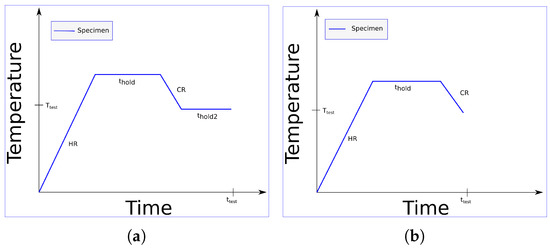
Figure 3.
A schematic representation of the two test series used to characterize the DSS in the thermal–mechanical simulator. represents the heating rate, is the cooling rate, is the holding time and is the holding time at the testing temperature . The detailed test parameters are given in Table 2. (a) The series describing the stationary microstructure after welding. (b) The series describing the non-stationary microstructure after welding.
In the first series of the thermal–mechanical experiments, see Figure 3a, the specimens were cooled from 1250 °C with a cooling rate to the testing temperature , held a certain time , strained to 0.03 mm/mm and subsequently quenched with water.
In the second series of the thermo-mechanical experiments, see Figure 3b, the specimen was cooled to the testing temperature and directly tested and quenched.
Due to the different test temperatures for the thermo-mechanical tests, the etching response of the samples to conventional etchants varied from one sample to another and no general preparation process could be found that could be used for all samples reliably.
Therefore, electron back scatter diffraction (EBSD) was used instead of conventional metallurgical etchings combined with microscopy to ensure consistent results of phase fractions and grain sizes that can be statistically analyzed.
Scanning electron microscopy was performed using a GeminiSEM 450 from Carl Zeiss SMT. EBSD measurements were carried out using the Symmetry® detection system from Oxford Instruments. During the conventional section preparation via grinding and polishing, a plastically deformed layer (approximately 5 nm thick) forms on the sample surface, which can interfere with the measurement signal during EBSD analysis. A silica oxide polish like an OP-S polish or ion polish, for example, works well to remove this layer. In this work, ion polishing was performed using the Ion Milling System IM 4000+ from Hitachi High-Technologies Europe GmbH with Ar ions. The samples were flat-milled for 3 min at an excitation voltage of 4 kV, an angle of incidence of about 10° and a sample rotation speed of 25 rpm. The EBSD scans were conducted with a step size of 30 nm. A cleanup of the data was performed using a grain dilatation angle of 10.5° and a minimum grain size of 2 pixels. The measurements were evaluated by means of the EDAX OIM Analysis™ software (V8.5) package.
For the microstructure evolution model for the phase i, the area-weighted diameter of the different phases as well as the phase fraction were of interest. and are defined as:
represents the area of the specified phase i.
represents the area of the grains where no edge grains were considered. represents the diameter of those grains and the total surface area of all the grains considered in the area.
The experimental methods used, as well as the results for the thermal properties of SAF2507, can be found in the Appendix B in Table A3.
2.4. Numerical Methods
In this section, the methods used for the microstructure evolution model and the fitting of the single-phase flow curves for ferrite and austenite, respectively, using a representative volume element (RVE) are described.
Microstructure Evolution Model
The developed microstructure evolution model is based on previous work by Hemmer et al. [16,21], which models the microstructure evolution of DSS during welding. The model contains some simplifications focusing on the essential aspects relevant for DSS welding simulations. This model can be categorized in the mesoscopic scale category and as such does not cover the exact microstructure changes that occur during welding DSSs, such as, for example, dendritic solidifications of ferrite in the fusion zone. As such, this model will describe different zones of welds with different levels of accuracy. The assumption that the weld metal inside the fusion zone of the weld behaves similar to the heat-affected zone is a simplification. The most important model features are the dissolution of austenite during heating, followed by a subsequent grain growth in the delta ferrite regime and finally the decomposition of delta ferrite to austenite during cooling.
For the sake of simplicity, two further assumptions were made in the model: all reactions occur in succession, rather than in parallel, and no nucleation was considered. This allows for the governing equations to be written as first-order (separable) differential equations, which read as follows:
and represent arbitrary functions of X and T, where X represents a state variable in dimensionless form and T represents the temperature. The function is a time constant that includes the temperature dependence of the reaction. An equation of the form of Equation (6) can be reduced to the well-known Scheil integral [22,23,24]. Following this approach, it becomes obvious that the transformation rates depend only on the current values of each kind of state variable, which means that there is no direct coupling between the microstructural field and the thermal field. This reduces the mathematical problem from a two-state variable problem to a single-state variable problem, making it a closed isokinetic problem, provided that the differential evolution equations contain separable variables. The following equations describe the microstructure evolution model as presented by [16,21].
Two effects are being described by Equation (7). The first term describes the dissolution of austenite during heating, with being the time constant for the dissolution. The second term of Equation (7) describes the back diffusion that happens if the austenite is not fully dissolved, with being a time constant for the back diffusion. f and are the current and initial volume fraction of austenite in the material.
Equations (8) and (9) model the delta ferrite grain growth both during and after the decomposition of the austenite phase. Y and represent the dimensionless scaling parameter used in the grain growth model, is the initial delta ferrite grain size after the complete dissolution of the austenite phase and n is the time exponent. A schematic representation of the different parts of the model is illustrated in Figure 1 of [16].
Equations (10) and (11) describe the decomposition of delta ferrite to austenite during cooling. is a parameter related to the thickness of the austenite shell, is the value of for the reference material and is the time constant in the delta ferrite decomposition model. Equation (11) predicts the volume fraction f of the austenite. This part of the model calculates the phase fraction assuming that the austenite formation will grow from the outside of, in the early stages assumed, a spherical ferrite grain. Thus, it is represented by the fraction of the volumes of those spheres; a graphical representation can be found in [16]. is the radius of the initial delta ferrite grain from which an austenitic shell with inner radius grows.
The programming language Python and a multi-objective optimizer package called pymoo [25] was used to fit the parameters of the microstructure-evolution model.
2.5. Representative Volume Element Approach for Determination of Single-Phase Flow Curves
The description of the mechanical material behavior of a material with changing phase composition demands single-phase material models for all involved phases. To calculate single-phase flow curves from experimentally determined two-phase flow curves, an RVE-modeling approach was used. With the RVE, it is possible to include micromechanics in the form of different volume fractions of phases as well as different microstructural characteristics [26]. It has been shown that a 2D plain strain hexagon RVE is a good approximation despite the pancake-like microstructure of the DSS [11,27]. A schematic representation of the used RVE is shown in Figure 2. Besides the volume fractions of the constituting phases, the necessary microstructural characteristics as the mean diameters of the different phases, as well as the mean intercept lengths are taken into account. The mean diameter was measured using the EBSD measurements of the cross sections of the samples created with the thermo-mechanical simulator; see Equation (5). The mean intercept lengths were converted from the measured mean diameter data assuming the spherical shape model [28]. The RVE contains measured phase fractions, which are evenly distributed by a randomization algorithm so as to achieve a truly “interwoven” status, which is typical of a duplex microstructure.
From the thermal–mechanical simulator, the two-phase flow curves were experimentally determined and, from the quenched specimen, the microstructural data were measured by means of EBSD.
The RVE implements a Hall–Petch formalism:
where represents the yield stress of either austenite or ferrite ; further, is the initial yield stress, the intercept lengths from the micrograph and the Hall–Petch constants [27].
The mechanical behavior of the phases was approximated using the Voce law, a non-linear isotropic hardening law [29]:
where represents the initial yield stress including the aforementioned Hall–Petch relation, the hardening parameter that governs the rate of the saturation in the exponential term, the exponential coefficient, the linear coefficient defining the slope of the saturation and the accumulated equivalent plastic strain.
Together with the experimental data from the Gleeble® tests, the two-phase flow curves and the measured temperatures, as well as the phase fractions and topological information from the EBSD measurements, the single-phase flow curves could be reverse-fitted using the RVE, analogous to [26,30].
3. Results and Discussion
In this section, the results of the previously mentioned methods are summarized and consequently discussed in relation to the model-building process. To avoid overloading the figures and tables, only the data points deemed relevant for discussion are shown and discussed in the following section. A complete set of the single-phase flow curves can be found in Section 3.3.
3.1. Two-Phase Flow Curves
The parameters for the experiments of the physical simulations are given in Table 2. and the two-phase flow curves for the experimental series of 700NHT and 700HT are shown as an example in Figure 4a.
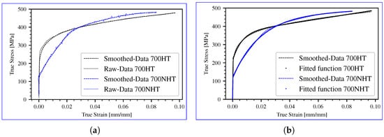
Figure 4.
(a) The measured and subsequently smoothed flow curves from the thermal–mechanical simulator for the testing series of 700NHT and 700HT. (b) The fitted two-phase flow curves for the testing series of 700NHT and 700HT using Equation (13). For the exact experimental parameters used, see Table 2.
The experimental flow curves determined by means of the thermo-mechanical simulator could be used to fit the plastic strains; however, due to the experimental set up and some variations due to the high heating rates, the elastic part of the flow curve could not be used for fitting. For the elastic part of the flow curve, the Young’s modulus and Poisson ratio were taken from JMatPro and from the literature [31,32,33,34].
Figure 4b shows the smoothed experimental data, as well as the fitted two-phase flow curve using the above mentioned non-linear isotropic hardening law; see Equation (13). These two-phase flow curves were used for the optimization using the RVE; see Section 3.3.
Figure 4b showcases the excellent agreement between the smoothed experimental data and the fitted two-phase flow curve, validating the accuracy of the model. This alignment serves as the baseline for the subsequent analysis in Section 3.3, where the single-phase flow curves are extracted to further enhance the understanding of the material behavior under different phase compositions and mean grain diameter.
3.2. Microstructure Evolution Model Results
The temperature–time curve used in the thermal–mechanical simulator experiments, especially the cooling and heating rates, correlates closely to actual welding experiments. In Figure 5, the results of the experimental series for 700 °C are shown together with two corresponding EBSD measurements. The measured phase fraction of the austenite f and the delta ferrite grain size were used for fitting the parameters of the microstructure evolution model.
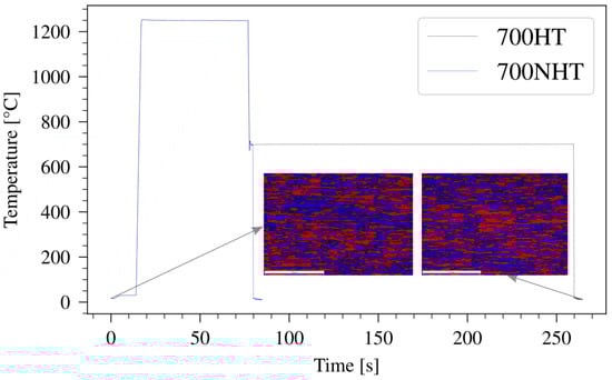
Figure 5.
Experimental results for 700 °C for both experimental series performed with the thermal–mechanical simulator. NHT represents the series without holding time before tensile testing. HT represents the series with holding time before testing. For details regarding the experimental parameters, see Table 2. At the bottom, EBSD results showing the - (red) and -phase fractions (blue) from two measurements, the initial state and the state after experiment 700NHT, are embedded.
During the optimization of these parameters, a Pareto front was calculated and, while examining the different parameter sets, a stronger emphasis was given to the accuracy of the calculation of the phase fraction. This was carried out because, from the point of view of a welding engineer, an error in the phase fraction could be more detrimental than an error in the grain size [3,35]. The results with the originally presented parameters, however, yielded a slight offset to the measured grain diameters, so an extra offset diameter was introduced; see Equation (14).
In the original paper by Hemmer and Grong [16,21], the results were within a 30% error margin. With the presented experiments, a variation of only 12% regarding the phase fraction and 25% regarding the mean grain diameter of ferrite was achieved; see Figure 6.
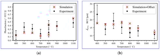
Figure 6.
(a,b) The calculated results of the microstructure evolution model compared to the measured results as determined from the thermal–mechanical simulator experiments. (a) It is shown that the calculated phase fraction of austenite in comparison to the experimental results from the thermo-mechanical simulator fit well within a 12% error margin with only one exception at 500 °C. (b) It is shown that the calculated mean grain diameter for ferrite matched within a 25% error margin, with one exception, to the experimental results from the thermo-mechanical simulator.
The introduction of the extra offset diameter refines the model and contributes to enhancing the accuracy of the predictions. Figure 6 clearly demonstrates a notable reduction in variation, underscoring the efficacy of the introduced parameter in achieving a closer match to the measured grain diameters.
3.3. Single-Phase Flow Curves
The RVE was used to reproduce the measured flow curves of the thermal–mechanical simulator; in conjunction with the experimental results from the EBSD experiments, as described in Section 2.5, it is possible to calculate the single-phase flow curves. Figure 7 shows the recalculated two-phase flow curve, see Figure 7a, as well as the calculated single-phase flow curves, see Figure 7b, for experiment 700NHT. All calculated single-phase flow curves from room temperature up to 1100 °C are given in Figure 8a for austenite and Figure 8b for ferrite.
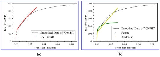
Figure 7.
The two subfigures show the calculated flow curves using the representative volume element (RVE) approach at 700 °C for the 700NHT experiment (refer to Table 2 for experimental details). In (a), the calculated two-phase flow curve is depicted alongside the smoothed data from the 700NHT experiment. Meanwhile, (b) illustrates the resulting single-phase flow curves for austenite and ferrite using the RVE approach.
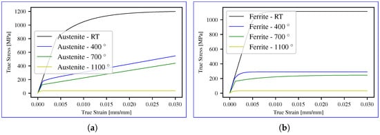
Figure 8.
The two subfigures show the calculated single-phase flow curves for austenite (a) and ferrite (b) calculated with the RVE approach, covering the temperature range from room temperature to 1100 °C.
The calculated flow curves were only defined up to mm/mm because the presented material model is used for welding and any strain above mm/mm from thermal dilatation or metallurgical strain is unlikely. The presented single-phase flow curves show similar characteristics through all temperature ranges: the austenite displays a higher ultimate strength with a lower yield strength as well as lower hardening compared to the ferrite. These findings are consistent with those observed in other studies investigating single-phase flow curves of duplex stainless steels [33,36,37,38].
4. Conclusions
A multi-scale approach was used to develop a fully parameterized constitutive thermal–mechanical–metallurgical material model for an FE-welding simulation. A thermal–mechanical simulator was used to perform tests with laboratory precision from room temperature up to 1100 °C, representing the thermal–mechanical loading situation for the different parts of a weld while excluding completely molten specimens. The microstructure of the tested specimens was analyzed by means of EBSD measurements. Combining the EBSD measurements and a microstructure evolution model based on the works of Hemmer and Grong [16,21], a model was developed that describes the relevant phase transformations of the investigated duplex steel. The comparison of experimental and calculated results shows a deviation of up to 12% for the phase fraction of austenite and up to 25% for the mean grain diameter of ferrite . The resulting error margins are within reason for the application and match the original authors closely. A 2D plain strain RVE was used to calculate single-phase flow curves from the two-phase flow curves measured with a Gleeble® thermal–mechanical simulator. The recalculated flow curves of the RVE are in good agreement with the measured flow curves. The derived single-phase flow curves are in good agreement with literature data for single-phase flow curves of duplex steels [33,36,37,38].
A complete set of parameters for the thermal–mechanical–metallurgical material model for SAF2507 over a temperature range from room temperature to 1100 °C is provided in Table A1 and Table A2 in the appendix. The focus of this paper is set to the mechanical and metallurgical aspects of modeling SAF2507 in a welding environment but, for the sake of completeness, the relevant thermal properties for a thermal simulation are listed in the appendix as well; see Table A3.
The complete material model is going to be used for welding process simulations, which allow us to predict the resulting welding-induced stresses as well as the resulting phase distributions and grain sizes of ferrite and austenite of SAF2507. The continued studies using this material model can support any industry welding SAF2507 to reduce its welding distortion as well as part failure due to an improper weld joint.
Author Contributions
M.P.: original draft preparation, writing and investigation; P.R.: investigation; W.E.: methodology; M.R.: review and editing; R.E.: supervision, review, editing and validation. All authors have read and agreed to the published version of the manuscript.
Funding
The authors would like to acknowledge the financing received from the Austrian Research Promotion Agency (FFG) through the projects 874596, 866208 and 880645, as well as the Berndorf Band GmbH.
Data Availability Statement
The data presented in this study are available on request from the corresponding author. The data are not publicly available due to complexity and company policy. The data would need to be provided with a corresponding explanation.
Acknowledgments
The experimental investigations were performed in close cooperation with the Material Center Leoben (MCL) and the Chair of Metal Forming at the Montanuniversität Leoben.
Conflicts of Interest
Authors Maximilian Prunbauer and Martin Rester were employed by the company Berndorf Band GmbH. Authors Peter Raninger, Werner Ecker and Reinhold Ebner were employed by the company Materials Center Leoben Forschung GmbH. The authors declare that the research was conducted in the absence of any commercial or financial relationships that could be construed as a potential conflict of interest. The authors declare that this study received funding from Berndorf Band GmbH. The funder was not involved in the study design, collection, analysis, interpretation of data, the writing of this article or the decision to submit it for publication.
Appendix A. Parameters for the Presented Model
In this section of the appendix, all of the fitted and calculated parameters for the material model for SAF2507 are summarized.
Table A1.
In this table, all parameters for the single-phase flow curves of ferrite and austenite are given. The E-modulus values are taken from a JMatPro 12 calculation.
Table A1.
In this table, all parameters for the single-phase flow curves of ferrite and austenite are given. The E-modulus values are taken from a JMatPro 12 calculation.
| Temperature [°C] | E-Modulus [MPa] | [MPa] | [MPa] | [MPa] | (b) [] | i |
|---|---|---|---|---|---|---|
| RT | 206,940 | 580 | 0 | 250 | 850 | |
| RT | 199,840 | 653 | 200 | 400 | 160 | |
| 400 | 194,445 | 64 | 0 | 100 | 1000 | |
| 400 | 164,357 | 75 | 12,000 | 25 | 650 | |
| 700 | 160,647 | 5 | 0 | 85 | 140 | |
| 700 | 142,970 | 10 | 10,000 | 55 | 20 | |
| 1100 | 109,560 | 0 | 0 | 35 | 4000 | |
| 1100 | 112,725 | 0 | 10 | 33 | 200 |
Table A2.
In this table, all the parameters for the microstructure evolution model that were fitted are summarized. and are the reference temperature and time for the dissolution model of the austenite. and are the reference temperature and time for the part of the model that describes the back diffusion. and are the reference temperature and time for the grain growth model. and are the reference parameters for the delta ferrite decomposition. is the added offset from Equation (14).
| [°C] | [s] | [°C] | [s] | [°C] | [s] | [°C] | [s] | [m] |
|---|---|---|---|---|---|---|---|---|
| 1705.17 | 10 | 1491.14 | 10.75 | 1420.26 | 13.8 | 1345.64 | 5.79 | 7 |
Appendix B. Thermal Properties of SAF2507
In this section of the appendix, the thermal properties of SAF2507 are given. All of the given values were measured using three different methods. The specific heat capacity was measured using differential scanning calorimetry (DSC) [39], the thermal conductivity was measured using the laser flash method [40] and the density was measured using Archimedes’s principle [41].
Table A3.
In this table, all relevant thermal properties of SAF2507 in the discussed thermal ranges are given, with being the specific heat capacity, the density and the thermal conductivity.
Table A3.
In this table, all relevant thermal properties of SAF2507 in the discussed thermal ranges are given, with being the specific heat capacity, the density and the thermal conductivity.
| Temperature [°C] | [J/gK] | [kg/m3] | [W/mK] |
|---|---|---|---|
| 20 | 0.46 | 7809 | 12.2 |
| 400 | 0.548 | 7684 | 18.1 |
| 700 | 0.628 | 7572 | 24 |
| 1100 | 0.693 | 7402 | 30.7 |
References
- Charles, J. Duplex stainless steels, a review after DSS’07 in Grado. Rev. Metall. 2008, 105, 155–171. [Google Scholar] [CrossRef]
- Hosseini, V.A.; Hurtig, K.; Karlsson, L. Effect of multipass TIG welding on the corrosion resistance and microstructure of a super duplex stainless steel. Mater. Corros. 2017, 68, 405–415. [Google Scholar] [CrossRef]
- de Lima, M.S.F.; de Carvalho, S.M.; Teleginski, V.; Pariona, M. Mechanical and Corrosion Properties of a Duplex Steel Welded using Micro-Arc or Laser. Mater. Res. 2015, 18, 723–731. [Google Scholar] [CrossRef]
- Goldak, J.; Alkhalghi, M. Computational Welding Mechanics; Springer: Berlin/Heidelberg, Germany, 2005. [Google Scholar]
- Radaj, D. Schweißprozesssimulation; DVS Verlag: Dusseldorf, Germany, 1999. [Google Scholar]
- Phillips, D.H. Welding Engineering; John Wiley & Sons: Hoboken, NJ, USA, 2016. [Google Scholar]
- Sharafi, S. Microstructure of Super-Duplex Stainless Steels. Ph.D. Thesis, Department of Materials Science and Metallurgy Pembroke Street Cambridge, University of Cambridge, Cambridge, UK, 1993. [Google Scholar]
- Nyström, M. Plastic deformation of duplex stainless steels with different amounts of ferrite. In Proceedings of the 4th International Conference-Duplex Stainless Steels 94, Glasgow, UK, 13–16 November 1994. [Google Scholar]
- Nilsson, J.O. Super duplex stainless steels. Mater. Sci. Technol. 1992, 8, 685–700. [Google Scholar] [CrossRef]
- Alvarez-Armas, I.; Degallaix-Moreuil, S. Duplex Stainless Steels; ISTE Ltd.: London, UK; John Wiley & Sons Inc.: Hoboken, NJ, USA, 2009. [Google Scholar]
- Knyazeva, M.; Pohl, M. Duplex Steels: Part I: Genesis, Formation, Structure. Metallogr. Microstruct. Anal. 2013, 2, 113–121. [Google Scholar] [CrossRef]
- Wessman, S.; Selleby, M. Evaluation of austenite reformation in duplex stainless steel weld metal using computational thermodynamics. Weld. World 2013, 58, 217–224. [Google Scholar] [CrossRef]
- Lukas, H.; Fries, S.G.; Sundman, B. Computational Thermodynamics; Cambridge University Press: Cambridge, UK, 2007. [Google Scholar] [CrossRef]
- Schaeffler, A.L. Constitution diagram for stainless steel weld metal. Met. Prog. 1949, 56, 680. [Google Scholar]
- Zhang, Z.; Han, Y.; Lu, X.; Zhang, T.; Bai, Y.; Ma, Q. Effects of N2 content in shielding gas on microstructure and toughness of cold metal transfer and pulse hybrid welded joint for duplex stainless steel. Mater. Sci. Eng. A 2023, 872, 144936. [Google Scholar] [CrossRef]
- Hemmer, H.; Grong, Ø. A Process Model for the Heat-Affected Zone Microstructure Evolution in Duplex Stainless Steel Weldments: Part I. the Model. Metall. Mater. Trans. A 1999, 30, 2915–2929. [Google Scholar] [CrossRef]
- Wang, X.; Chen, W.; Zheng, H. Influence of isothermal aging on σ precipitation in super duplex stainless steel. Int. J. Miner. Metall. Mater. 2010, 17, 435–440. [Google Scholar] [CrossRef]
- Nilsson, J.O.; Wilson, A. Influence of isothermal phase transformations on toughness and pitting corrosion of super duplex stainless steel SAF 2507. Mater. Sci. Technol. 1993, 9, 545–554. [Google Scholar] [CrossRef]
- Knyazeva, M.; Pohl, M. Duplex Steels. Part II: Carbides and Nitrides. Metallogr. Microstruct. Anal. 2013, 2, 343–351. [Google Scholar] [CrossRef]
- Calliari, I.; Ramous, E.; Bassani, P. Phase Transformation in Duplex Stainless Steels after Isothermal Treatments, Continuous Cooling and Cold Working. Mater. Sci. Forum 2010, 638, 2986–2991. [Google Scholar] [CrossRef]
- Hemmer, H.; Klokkehaug, S.; Grong, Ø. A process model for the heat-affected zone microstructure evolution in duplex stainless steel weldments: Part II. Application to electron beam welding. Metall. Mater. Trans. A 2000, 31, 1035–1048. [Google Scholar] [CrossRef]
- Scheil, E. Anlaufzeit der Austenitumwandlung. Arch. EisenhüTtenwes. 1935, 8, 565–567. [Google Scholar] [CrossRef]
- Cahn, J.W. Transformation kinetics during continuous cooling. Acta Metall. 1956, 4, 572–575. [Google Scholar] [CrossRef]
- Christian, J. The Theory of Transformations in Metals and Alloys; Pergamon Press an Imprint of Elsevier Science: Oxford, UK, 2002; ISBN 0-08-044019-3. [Google Scholar]
- Blank, J.; Deb, K. Pymoo: Multi-Objective Optimization in Python. IEEE Access 2020, 8, 89497–89509. [Google Scholar] [CrossRef]
- Schemmel, M.; Prevedel, P.; Schöngrundner, R.; Ecker, W.; Antretter, T. Modelling of phase transformations and residual stress formation in hot-work tool steel components. In Proceedings of the European Conference on Heat Treatment and 21st IFHTSE Congress, Munich, Germany, 12–15 May 2014; pp. 285–292. [Google Scholar]
- Siegmund, T.; Werner, E.; Fischer, F. Structure-property relations in duplex materials. Comput. Mater. Sci. 1993, 1, 234–240. [Google Scholar] [CrossRef]
- ASTM. Standard Test Methods for Determining Average Grain Size; ASTM: West Conshohocken, PA, USA, 2013. [Google Scholar]
- Voce, E. A practical strain-hardening function. Metallurgia 1955, 51, 219–226. [Google Scholar]
- Tasan, C.; Diehl, M.; Yan, D.; Bechtold, M.; Roters, F.; Schemmann, L.; Zheng, C.; Peranio, N.; Ponge, D.; Koyama, M.; et al. An Overview of Dual-Phase Steels: Advances in Microstructure-Oriented Processing and Micromechanically Guided Design. Annu. Rev. Mater. Res. 2015, 45, 391–431. [Google Scholar] [CrossRef]
- Li, X.; Miodownik, P.; Saunders, N. Modelling of materials properties in duplex stainless steels. Mater. Sci. Technol. 2002, 18, 861–868. [Google Scholar]
- Eckart, E.; Meyer-Nolkemper, H.; Saeed, I. Fließkurvenatlas Metallischer Werkstoffe; HANSER: Vienna, Austria, 1986. [Google Scholar]
- Guo, E.Y.; Xie, H.X.; Singh, S.S.; Kirubanandham, A.; Jing, T.; Chawla, N. Mechanical characterization of microconstituents in a cast duplex stainless steel by micropillar compression. Mater. Sci. Eng. A 2014, 598, 98–105. [Google Scholar] [CrossRef]
- He, Y.; Liu, J.; Qiu, S.; Deng, Z.; Yang, Y.; McLean, A. Microstructure and high temperature mechanical properties of as-cast FeCrAl alloys. Mater. Sci. Eng. A 2018, 726, 56–63. [Google Scholar] [CrossRef]
- Zhang, Z.; Zhang, H.; Hu, J.; Qi, X.; Bian, Y.; Shen, A.; Xu, P.; Zhao, Y. Microstructure evolution and mechanical properties of briefly heat-treated SAF 2507 super duplex stainless steel welds. Constr. Build. Mater. 2018, 168, 338–345. [Google Scholar] [CrossRef]
- Tao, P.; Gong, J.M.; Wang, Y.F.; Jiang, Y.; Li, Y.; Cen, W.W. Characterization on stress-strain behavior of ferrite and austenite in a 2205 duplex stainless steel based on nanoindentation and finite element method. Results Phys. 2018, 11, 377–384. [Google Scholar] [CrossRef]
- Huang, Y.; Young, B. Stress–strain relationship of cold-formed lean duplex stainless steel at elevated temperatures. J. Constr. Steel Res. 2014, 92, 103–113. [Google Scholar] [CrossRef]
- Seol, D.J.; Won, Y.M.; Jung Yeo, T.; Oh, K.H.; Park, J.K.; Yim, C.H. High Temperature Deformation Behavior of Carbon Steel in the Austenite and δ-Ferrite Regions. ISIJ Int. 1999, 39, 91–98. [Google Scholar] [CrossRef][Green Version]
- EN 821-3:2005; Advanced Technical Ceramics-Monolithic Ceramics-Thermo-Physical Properties-Part 3: Determination of Specific Heat Capacity. Deutsches Institut für Normung (DIN): Berlin, Germany, 2005. [CrossRef]
- EN 821-2:1997; Advanced Technical Ceramics-Monolithic Ceramics, Thermo-Physical Properties-Part 2: Determination of Thermal Diffusity by the Laser Flash (or Heat Pulse) Method. Deutsches Institut für Normung (DIN): Berlin, Germany, 1997. [CrossRef]
- EN 993-11:2007; Methods of Test for Dense Shaped Refractory Products-Part 11: Determination of Resistance to Thermal Shock. Deutsches Institut für Normung (DIN): Berlin, Germany, 2004. [CrossRef]
Disclaimer/Publisher’s Note: The statements, opinions and data contained in all publications are solely those of the individual author(s) and contributor(s) and not of MDPI and/or the editor(s). MDPI and/or the editor(s) disclaim responsibility for any injury to people or property resulting from any ideas, methods, instructions or products referred to in the content. |
© 2024 by the authors. Licensee MDPI, Basel, Switzerland. This article is an open access article distributed under the terms and conditions of the Creative Commons Attribution (CC BY) license (https://creativecommons.org/licenses/by/4.0/).