Numerical Simulation of Macro-Segregation Phenomena in Transition Blooms with Various Carbon Contents

Abstract

This paper presents a numerical simulation of the steel grade transition from the ladle nozzle to the solidification end of the bloom. The simulation is based on models encompassing fluid flow, solidification, heat transfer, an electromagnetic field, and solute transport. To validate the accuracy of the steel grade transition model, transition blooms of high-carbon steel are sampled. Subsequently, the model is applied to investigating the steel grade transition between medium-carbon steel and low-carbon steel. The findings indicate that the regions exhibiting significant differences between their molten steel flow velocity and bloom casting speed in the strand model are primarily concentrated within 1 m below the meniscus. Additionally, the mushy zone in the strand model possesses a substantial volume. Solute elements continuously permeate the liquid phase from the solid phase through the mushy zone. Consequently, the distribution of solute elements in the transition bloom is primarily influenced by the molten steel flow in the tundish and macro-segregation in the casting process. The segregation degree of each solute element varies among grades with different carbon contents. In the austenite phase, the segregation degree of each element follows the order C > Si > Mo > Mn > Cr > Ni, while in the ferrite phase, the segregation degree is ordered as C > Si = Mn. Considering macro-segregation, the transition bloom partition model proves to be more stringent than the original partition method. This results in longer transition blooms when a significant difference exists between the new and old grades. For example, in Scheme 1, the original plan transition bloom length is 8.88 m, whereas the new plan transition bloom length is 10.88 m. Similarly, in Scheme 2, the original plan transition bloom length is 34.64 m, and the new plan transition bloom length is 35.16 m. Conversely, shorter partition intervals occur when there is an overlap in the composition of the new and old grades. In Scheme 3, the original plan partition interval for the new and old grades is 4.08 m, while the new plan partition interval is reduced to 0.94 m.

1. Introduction

In contemporary times, scholars have introduced a multitude of steel grades to accommodate diverse application scenarios. Some of these specialized steel materials boast high added value but experience relatively low demand, rendering it impractical to fulfill the requirements of a single casting sequence. In response to this challenge, the technology of steel grade transition has been proposed, enabling the production of different grades within the same casting sequence. However, the transition from one steel grade to another gives rise to transition blooms situated between the new and old grades. Consequently, reducing the length of the transition blooms and accurately predicting their positions have emerged as pivotal areas of focus in current research endeavors.

Numerous scholars have endeavored to minimize the length of the transition blooms by adjusting the molten steel flow field within the tundish and mold. Research by Siddiqui and Kim [1] suggests that the shortest transition billet can be achieved when the ladle nozzle is submerged to a depth of 38%, the inner wall angle of the turbulence inhibitor is 60°, the baffle height is 0.45 m, and the baffle is positioned 0.7 m away from the center of the tundish. In a study by Kumar et al. [2], an optimal baffle height was proposed as a means to reduce the length of the transition blooms. Siddiqui and Jha [3] found that the use of turbulence inhibitors could extend the length of the transition blooms. Agarwal et al. [4] discovered that closing one strand near the ladle nozzle would result in the longest transition billet. However, when closing two strands, shutting the strands near the ladle nozzle leads to the shortest transition billet.

In a strand model, Michalek et al. [5] conducted a comprehensive investigation into the impact of Submerged Entry Nozzle (SEN) structures on the length of round transition blooms. The findings suggest that the utilization of a straight-through-type SEN results in the production of the longest round transition blooms. Huang and Thomas [6,7,8] employed a three-dimensional (3D) plus one-dimensional numerical simulation of the strand to examine the composition distribution of transition slabs. The accuracy of this model was validated using industrial experimental data from Inland Steel.

The disparities in composition between the surface and center of transition blooms arise from the flow of molten steel and macro-segregation during the solidification process of the transition blooms. Failure to control central segregation and subsurface negative segregation in the bloom can result in the extended length of the transition bloom. Rappaz et al. [9,10,11] studied the formation, fragmentation, and remelting of dendrites during metal solidification. In recent years, scholars have developed macro-segregation models for blooms [12,13,14,15,16]. Szmyd and Suzuki [17] proposed a more accurate solute redistribution model, which improved the accuracy of the metal solidification model. Incorporating the composition of molten steel mixed through the tundish into the conventional strand model enables the study of the distribution of solute elements within the transition bloom.

In many Chinese steel enterprises employing steel grade transition technology, it is predominantly utilized for new and old grades with overlapping compositions. However, with the escalating competition in the market, instances of steel grade transition involving significant differences in composition between new and old grades have gradually risen. The previous research on the steel grade transition among high-carbon steels, medium-carbon steels, and low-carbon steels is relatively limited, with minimal exploration from the perspective of the macro-segregation of solute elements in the steel grade transition. This paper primarily concentrates on the steel grade transition of high-carbon steels. Through the establishment of numerical simulations encompassing fluid flow, heat transfer, solidification, an electromagnetic field, and solute transport, the distribution of solute elements in transition blooms is examined. The research findings are subsequently extrapolated to medium-carbon steels and low-carbon steels. The numerical simulation developed in this paper for predicting the distribution of solute elements in transition blooms represents a more precise transition bloom prediction model. Using this model, methods for reducing the length of the transition blooms are proposed.

2. Simulation Model

2.1. Model Description and Assumptions

This paper employed Fluent to conduct the numerical simulations, examining the complete steel grade transition process from the ladle shroud to the solidification endpoint of the bloom. A schematic diagram of the geometric model is illustrated in Figure 1. The exits of the tundish are designated as a “far SEN” and a “near SEN”. To prevent the entrainment of tundish powder in the molten steel, the tundish level should be controlled within the range of 810 mm to 560 mm. Furthermore, mold electromagnetic stirring (M-EMS) intensifies the formation of subsurface negative segregation in the bloom, while Final Electromagnetic Stirring (F-EMS) can alleviate central segregation in the bloom. Therefore, to diminish composition differences in the cross-section of the bloom and further reduce the length of the transition blooms, the study disabled M-EMS and only activated F-EMS.

Huang and Thomas [18] proposed that the solute transport induced by turbulent flow in the tundish is orders of magnitude greater than molecular diffusion. Therefore, it can be assumed that the differences in the liquid-phase diffusion coefficients of different solute elements in the molten steel can be neglected. This allows the treatment of new and old grades as separate components to study the steel grade transition in the tundish. The numerical simulations of the tundish flow field [19,20,21,22,23,24,25] and numerical simulations of the F-EMS electromagnetic field [26,27,28,29,30] have become relatively mature. This paper does not delve further into the modeling process for the tundish steel grade transition and F-EMS.

The steel grade transition of a bloom encompasses various intricate physical phenomena, including fluid flow, heat transfer, solidification, an electromagnetic field, and solute transport. It is crucial to take into account the influence of the macro-segregation of solute elements on the length of the transition blooms. Therefore, when calculating the steel grade transition of a bloom, it becomes necessary to convert the dimensionless concentration of the new grade at the SEN in the tundish model into the mass fraction $C_{t,spe}$ of each solute element using Equation (1).

$$C_{t,spe}=F(C_{n,spe}-C_{o,spe})+C_{o,spe}$$

(1)

where $C_{n,spe}$ and $C_{o,spe}$ represent the mass fractions of the solute elements in the new and old grades, respectively. After the conversion, it needs to be written into a Profile file and then imported into the SEN of the strand model. The parameters of the strand model are shown in

Table 1. Parameters of continuous caster.

Parameter	Value	Unit	Parameter	Value	Unit
Ladle shroud inner diameter	75	mm	SEN inner diameter	45	mm
Ladle shroud outer diameter	148	mm	SEN outer diameter	95	mm
Ladle shroud submerged depth	350	mm	Submerged depth of SEN	150	mm
Casting speed	1.2	m/min	Bloom cross-section	240 × 240	mm2
Mold length	700	mm	Loop 0 length	400	mm
Loop 1 length	2100	mm	Loop 2 length	2600	mm
Loop 3 length	3200	mm	Loop 4 length	15,000	mm
F-EMS current intensity	400	A	F-EMS frequency	4	Hz
F-EMS core inner diameter	660	mm	F-EMS core outer diameter	800	mm
F-EMS coil height	600	mm	F-EMS inner diameter	500	mm
F-EMS core height	500	mm	F-EMS center position from meniscus	17,000	mm

.

The steel grade transition involves multiple complex physical phenomena, encompassing fluid flow, heat transfer, solidification, an electromagnetic field, and solute transport. It is important to note that numerical simulations cannot perfectly replicate real-world conditions. To streamline the numerical simulation process, this paper makes the following assumptions:

• The new and old grades are considered transient, turbulent, and incompressible Newtonian fluids. The density of the molten steel is calculated using the volume-weighted mixing law within the tundish. After mixing in the tundish, it is assumed that the density of the new and old grades does not undergo a sudden change. The density of the molten steel entering the mold follows the Boussinesq assumption. Assuming that the density of the new and old grades entering the mold is constant, both are 7020 kg/m³.
• The simulation only considers the Fe elements in the new and old grades and some solute elements with higher mass fractions.
• The mushy zone is treated as a porous medium, and the flow within the mushy zone follows Darcy’s law.
• The effects of the solidification shrinkage of the molten steel and the curvature of the continuous caster on the solidification process of the bloom are neglected.
• The solid-state phase change latent heat, which is far less than the latent heat of solidification, is also ignored.
• Induction magnetic fields and the induced heat in the molten steel, as well as the impact of the molten steel flow on the magnetic field, are disregarded. Average electromagnetic forces are used instead of transient values.

2.2. Governing Equations

2.2.1. Fluid Flow

The Navier–Stokes equation and the momentum equation are as follows [31]:

$$\partial \rho /\partial t+\nabla \cdot \left(\rho \overrightarrow{v}\right)=0$$

(2)

$$\frac{\partial \left(\rho \overrightarrow{v}\right)}{\partial t}+\nabla \cdot \left(\rho \overrightarrow{v}\overrightarrow{v}\right)=-\nabla p+\mu \nabla \cdot \left(\nabla \overrightarrow{v}+\nabla {\overrightarrow{v}}^T\right)+\rho \overrightarrow{g}+F_T+F_c+S_D+F_{mag}$$

(3)

$$F_T=\rho \overrightarrow{g}{\beta }_T\left(T-T_{ref}\right)$$

(4)

$$F_c=\rho \overrightarrow{g}\sum _{i=0}^{N_s}{\beta }_{C,spe}\left(C_{spe}-C_{ref,spe}\right)$$

(5)

$$S_D=\frac{(1-\beta {)}^2}{\left({\beta }^3+{\beta }_0\right)}{A}_{\mathrm{mush} }\left(\overrightarrow{v}-{\overrightarrow{v}}_c\right)$$

(6)

where $\rho$ is the density, $t$ is the time, $\overrightarrow{v}$ is the velocity, $p$ is the static pressure, $\mu$ is the laminar viscosity, $\overrightarrow{g}$ is gravity with a value of 9.81 m/s², $F_T$ is the thermal buoyancy, $F_c$ is the solute buoyancy, $S_D$ is the momentum sinking described in Darcy’s law, $F_{mag}$ is the electromagnetic force, ${\beta }_T$ is the thermal expansion coefficient with a value of 0.0002 K⁻¹, $T$ is the temperature, $T_{ref}$ is the reference temperature, $N_s$ is the number of solute types other than Fe, ${\beta }_{C,spe}$ is the solutal expansion coefficient of the species ${spe}^{th}$, $C_{spe}$ is the mass fraction of the species ${spe}^{th}$, $C_{ref,spe}$ is the reference mass fraction of the species ${spe}^{th}$, $\beta$ is the liquid fraction, ${\beta }_0$ is a small number to prevent division by zero with a value of 0.001, $A_{\mathrm{mush}}$ is the mushy zone constant with a value of 1.0 × 10⁸ [32], and ${\overrightarrow{v}}_c$ is the casting velocity.

The turbulence model used in the article is Standard $k-\epsilon$. The turbulent flow energy, $k$, is represented as follows:

$$\frac{\partial \left(\rho k\right)}{\partial t}+\rho k\frac{\partial \left(v_i\right)}{\partial x_i}=\frac{\partial }{\partial x_j}\left[\left(\mu +\frac{{\mu }_t}{{\sigma }_k}\right)\frac{\partial k}{\partial x_j}\right]+{\mu }_t\left(\frac{\partial v_i}{\partial x_j}+\frac{\partial v_j}{\partial x_i}\right)\frac{\partial v_i}{\partial x_j}-\rho \epsilon +S_k$$

(7)

$$S_k=\frac{(1-\beta {)}^2}{\left({\beta }^3+{\beta }_0\right)}{A}_{\mathrm{mush} }k$$

(8)

The dissipation rate, $\epsilon$, of $k$ is represented as follows:

$$\frac{\partial }{\partial t}\left(\rho \epsilon \right)+\frac{\partial }{\partial x_i}\left(\rho \epsilon v_i\right)=\frac{\partial }{\partial x_j}\left[\left(\mu +\frac{{\mu }_t}{{\sigma }_{\epsilon }}\right)\frac{\partial \epsilon }{\partial x_j}\right]+C_{1\epsilon }\frac{\epsilon }{k}{\mu }_t\left(\frac{\partial v_i}{\partial x_j}+\frac{\partial v_j}{\partial x_i}\right)\frac{\partial v_i}{\partial x_j}-C_{2\epsilon }\rho \frac{{\epsilon }^2}{k}+S_{\epsilon }$$

(9)

$$S_{\epsilon }=\frac{(1-\beta {)}^2}{\left({\beta }^3+{\beta }_0\right)}{A}_{\mathrm{mush} }\epsilon$$

(10)

The turbulent flow energy, $k$, is represented as follows:

$${\mu }_t=\rho C_{\mu }\frac{k^2}{\epsilon }$$

(11)

where $C_{1\epsilon }$, $C_{2\epsilon }$, and $C_{\mu }$ are constants with values of 1.44, 1.92, and 0.09, respectively; $S_k$ and $S_{\epsilon }$ are the sinks induced in the mushy and solidified zones; and ${\sigma }_k$ and ${\sigma }_{\epsilon }$ are the turbulent Prandtl numbers for $k$ and $\epsilon$, with values of 1.00 and 1.30, respectively [33].

2.2.2. Solidification and Heat Transfer

The energy equations are written as:

$$\frac{\partial }{\partial t}\left(\rho H\right)+\frac{\partial \left(\rho v_{i}H\right)}{\partial x_i}=\frac{\partial }{\partial x_i}\left(\lambda \frac{\partial T}{\partial x_i}\right)$$

(12)

$$H=h_{ref}+{\int }_{T_{ref}}^T{c}_{p}dT+\beta L_{lat}$$

(13)

where $H$ is the enthalpy, $\lambda$ is the laminar thermal conductivity, $h_{ref}$ is the reference enthalpy, $c_p$ is the specific heat, and $L_{lat}$ is the latent heat.

2.2.3. Species Transfer

The micro-segregation model in this article adopts the lever rule, and the conservation equations for species transfer are described as follows:

$$\frac{\partial }{\partial t}\left(\rho C_{spe}\right)+\nabla \cdot \left(\rho S_c\right)=-\nabla \cdot {\overrightarrow{J}}_{spe}$$

(14)

$$S_c=\beta \frac{\left(\overrightarrow{v}-{\overrightarrow{v}}_c\left(1-\beta \right)\right)}{\beta }{C}_{spe}+\left(1-\beta \right){\overrightarrow{v}}_c{K}_{spe}{C}_{spe}$$

(15)

$${\overrightarrow{J}}_{spe}=-\rho \left[\beta D_{spe,liq}\nabla C_{spe}+(1-\beta )D_{spe,sol}\nabla K_{spe}{C}_{spe}\right]$$

(16)

where $S_c$ is the product of velocity and mass fraction, and ${\overrightarrow{J}}_{spe}$ is the diffusion flux of species ${spe}^{th}$, $K_{spe}$ is the partition coefficient of the species ${spe}^{th}$, and $D_{spe,liq}$ and $D_{spe,sol}$ are the liquid-phase diffusion coefficient and the solid-phase diffusion coefficient, respectively.

The liquid fraction, $\beta$, is described as:

$$\beta =\left\{\begin{array}{c}1\hspace{1em}\hspace{1em}\hspace{1em}\hspace{1em}\mathrm{i}\mathrm{f} T\ge T_{\mathit{liq} }\hfill \\ \frac{T - T_{\mathit{sol}}}{T_{\mathit{liq} }- T_{\mathit{sol}}}\hspace{1em}\mathrm{i}\mathrm{f} T_{\mathit{liq} }\ge T\ge T_{\mathit{sol}}\hfill \\ 0\hspace{1em}\hspace{1em}\hspace{1em}\hspace{1em}\mathrm{i}\mathrm{f} T\le T_{\mathit{sol}}\hfill \end{array}\right\}$$

(17)

The liquidus temperatures $T_{\mathit{liq}}$ and the solidus temperatures $T_{\mathit{sol}}$ are described as:

$$T_{\mathit{liq} }=T_{\mathit{melt}}+\sum _{\mathit{solutes}}{m}_{spe}{C}_{spe}$$

(18)

$$T_{\mathit{sol}}=T_{\mathit{melt} }+\sum _{\mathit{solutes}}{m}_{spe}{C}_{spe}/K_{spe}$$

(19)

where $m_{spe}$ is the slope of the liquidus surface of the species ${spe}^{th}$, and $T_{\mathit{melt}}$ is the melting temperature of pure iron with a value of 1808 K.

2.3. Boundary Conditions

The boundary conditions for this simulation are as follows:

1.

The SEN is defined as a velocity inlet with a velocity magnitude of 0.72 m/s. The turbulence intensity $I$ is calculated using Equation (20), with a value of 0.043.

$$I=0.016{\left(\frac{\rho v{D}_{SEN}}{\mu }\right)}^{-0.125}$$

(20)

where $D_{SEN}$ represents the inner diameter of the SEN.

2.

The outlet for the strand model is set as outflow.

3.

All the other boundaries are designated as walls.

For the steel–slag interface, the shear stress is set to 0, and the heat transfer at the steel–slag interface is ignored. The walls surrounding the domain have a velocity matching the casting speed, and the heat transfer conditions are defined for various sections of the strand. The heat transfer conditions are set as follows:

-

Mold zone. The heat flux density $q_{mold}$ in the mold zone is calculated using Equation (21).

$$q_{mold}=\mathrm{2,688,000}-(\mathrm{4,020,000}-\frac{1.5\times {c_p}_{water}\times m\times \mathsf{\Delta }{T}_{water}}{S_{eff}})\sqrt{\frac{L_{men}}{L_{mold}}}$$

(21)

where $L_{men}$ is the distance from the meniscus surface, $L_{mold}$ is the effective length of the mold, ${c_p}_{water}$ is the specific heat capacity of the cooling water, $m$ is the flow rate of the cooling water in the mold, $\mathsf{\Delta }{T}_{water}$ is the temperature difference in the cooling water in the mold, and $S_{eff}$ is the effective cooling area of the mold.

-

Secondary cooling zone. The heat flux density in the secondary cooling zone is represented by $q_{foot}$ and $q_{other}$ in the foot roll zone and the other zones, respectively.

$$q_{foot}=420w_{foot}^{0.351}\times (T_{sur}-T_{water})$$

(22)

$$q_{other}=(116+10.44w_{other}^{0.851})\times (T_{sur}-T_{water})$$

(23)

where $T_{sur}$ represents the surface temperature of the bloom, and $T_{water}$ represents the temperature of the cooling water. The parameters of the secondary cooling zone are shown in

Table 2. Parameters of the secondary cooling zone.

Loop Number	Water Flow Rate (L/(m2·s))	Convection Coefficient (W/(m2·K))	Loop Number	Water Flow Rate (L/(m2·s))	Convection Coefficient (W/(m2·K))
0	63.5	1803.1	1	105.0	664.0
2	53.6	425.0	3	19.4	246.0

:

-

Air-cooling zone. The heat flux density $q_{air}$ in the air-cooling zone is calculated using Equation (24) [34].

$$q_{air}={\sigma }_{SB}{\epsilon }_{bla}\left(T_{sur}^4-T_{amb}^4\right)$$

(24)

where ${\sigma }_{SB}$ is the Stefan–Boltzmann constant with a value of 5.67 × 10⁻⁸ W/(m²·K), ${\epsilon }_{bla}$ is the blackness at the bloom surface with a value of 0.8, and $T_{amb}$ is the ambient temperature with a value of 300 K.

2.4. Material Parameters and Simulation Schemes

Research indicates that opting for steel grades with a lower density as the new grade can lead to shorter transition blooms [35]. In this paper, it is assumed that the physical properties of the mixed molten steel flowing from the tundish into the mold remain constant, with the specific parameters detailed in

Table 3. The material parameters in the strand model.

Parameter	Value	Unit	Parameter	Value	Unit
Specific heat of steel	650	J/(kg·K)	Viscosity of steel	0.0062	kg/(m·s)
Pure solvent melting heat	270,000	J/kg	Thermal conductivity	41	W/(m·K)
Liquid-phase diffusion coefficient	2.0 × 10−9	cm2/s

. Additionally,

Table 4. Composition range and actual composition of new and old grades.

Grage	C	Si	Mn	Cr	Ni	Mo
Old grade GCr15 range	0.95~1.05	0.15~0.35	0.25~0.45	0.95~1.05	≤0.20	-
Old grade GCr15 composition	1.00	0.29	0.36	0.99	0.01	-
New grade GCr15SiMn range	0.95~1.05	0.40~0.65	0.90~1.20	1.30~1.65	≤0.20	-
New grade GCr15SiMn composition	0.99	0.46	0.98	1.37	0.01	-
Old grade 30Cr2Ni2Mo range	0.26~0.34	0.17~0.37	0.30~0.60	1.80~2.20	1.80~2.20	0.50~0.80
Old grade 30Cr2Ni2Mo composition	0.31	0.23	0.52	2.1	2.08	0.68
New grade 30CrNi3Mo range	0.30~0.40	0.17~0.37	0.50~0.80	1.10~1.70	2.75~3.25	0.25~0.40
New grade 30CrNi3Mo composition	0.33	0.26	0.58	1.32	2.82	0.31
Old grade Q345 range	0.13~0.16	≤0.40	1.20~1.35	≤0.30	≤0.03	≤0.08
Old grade Q345 composition	0.15	0.31	1.25	0.01	0.01	0.03
New grade Q355 range	0.13~0.17	≤0.47	1.30~1.55	≤0.30	≤0.03	≤0.10
New grade Q355 composition	0.15	0.28	1.5	0.01	0.01	0.02

provides the composition ranges and actual compositions of three pairs of steel grades utilized in the steel grade transition.

The solidification process of the three pairs of steel grades used in the steel grade transition is depicted in Figure 2. The material parameters for the solute elements corresponding to each steel grade are set based on the iron–carbon phase diagram. Specifically, when Q345 is the old grade and Q355 is the new grade, the parameters for each solute element in the ferrite phase are applied. When GCr15 is the old grade and GCr15SiMn is the new grade, the parameters for each solute element in the austenite phase are utilized. For the pair with 30Cr2Ni2Mo as the old grade and 30CrNi3Mo as the new grade, the parameters for each solute element in the ferrite phase are used at temperatures above 1495 °C (1768 K), and the parameters for each solute element in the austenite phase are used at temperatures below 1495 °C (1768 K). These parameters are imported into the strand model using a user-defined function.

Table 5. Species-dependent thermophysical properties [36,37].

Element	${\mathit{K}}_{\mathit{\delta },\mathit{s}\mathit{p}\mathit{e}}$	${\mathit{K}}_{\mathit{\gamma },\mathit{s}\mathit{p}\mathit{e}}$	${\mathit{D}}_{\mathit{\delta },\mathit{s}\mathit{p}\mathit{e},\mathit{s}\mathit{o}\mathit{l}}$ (cm2/s)	${\mathit{D}}_{\mathit{\gamma },\mathit{s}\mathit{p}\mathit{e},\mathit{s}\mathit{o}\mathit{l}}$ (cm2/s)	${\mathit{m}}_{\mathit{s}\mathit{p}\mathit{e}}$ (K/wt.%)	${\mathit{\beta }}_{\mathit{C}}$ (1/wt.%)
C	0.19	0.34	0.0127exp(−19,450/RT)	0.0761exp(−32,160/RT)	78.0	1.10 × 10−2
Si	0.77	0.52	8.0exp(−59,500/RT)	0.3exp(−60,100/RT)	7.6	1.19 × 10−2
Mn	0.77	0.785	0.76exp(−53,640/RT)	0.055exp(−59,600/RT)	4.9	1.92 × 10−3
Cr	0.95	0.86	2.4exp(−57,310/RT)	0.0012exp(−52,340/RT)	1.04	3.97 × 10−3
Ni	0.83	0.95	1.6exp(−57,360/RT)	0.34exp(−67,490/RT)	4.69	−6.85 × 10−4
Mo	0.8	0.585	3.47exp(−57,690/RT)	0.068exp(−59,000/RT)	2.6	−1.92 × 10−3

provides a detailed list of parameters related to the solute elements for the new and old grades, where R is the gas constant, and its value is 1.987 cal/(mol·K).

The relatively small partition coefficient of the C element leads to a higher C segregation. Moreover, the large slope of the liquidus surface for the C element results in the liquidus line temperature being significantly influenced by the mass fraction of the C element in the molten steel. Therefore, in the steel grade transition, it is advisable to choose steel grades with similar mass fractions of the C element. The research schemes in this paper are outlined in

Table 6. Numeric simulation schemes.

No.	Old Grade	New Grade	Tundish Level	No.	Old Grade	New Grade	Tundish Level
1	GCr15	GCr15SiMn	560 mm	2	30Cr2Ni2Mo	30CrNi3Mo	560 mm
3	Q345	Q355	560 mm	4	GCr15	GCr15SiMn	810 mm
5	GCr15	GCr15SiMn	0 mm

, where Schemes 1, 2, and 3 correspond to steel grade transition between pairs of high-carbon steels, medium-carbon steels, and low-carbon steels, respectively. Schemes 4, 1, and 5 investigate steel grade transitions with different tundish levels. When using the flying tundish technology, the new and old grades are not mixed in the tundish, so the tundish level of Scheme 5 is 0 mm.

3. Results and Discussion

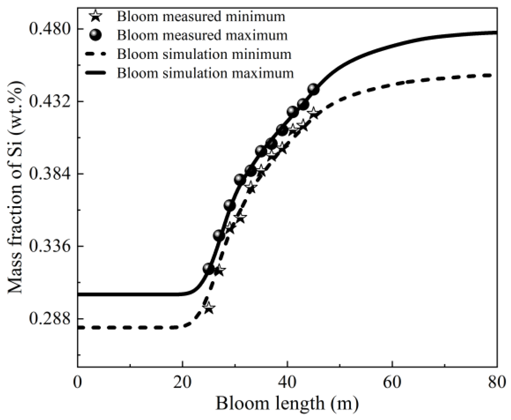
3.1. Model Validation

In spectral analysis, it was found that the variation pattern of the C element was not obvious [6], so this paper measured the mass fraction of the Si element. Figure 3 illustrates the simulated and measured Si content in the transition bloom when GCr15 serves as the old grade and GCr15SiMn as the new grade. The sampling positions for the transition bloom include the subsurface negative segregation zone and the central segregation zone, with a sampling interval of 2 m. The excellent consistency between the measured data and the simulated data confirms the accuracy of the model.

3.2. Foundation before Steel Grade Transition

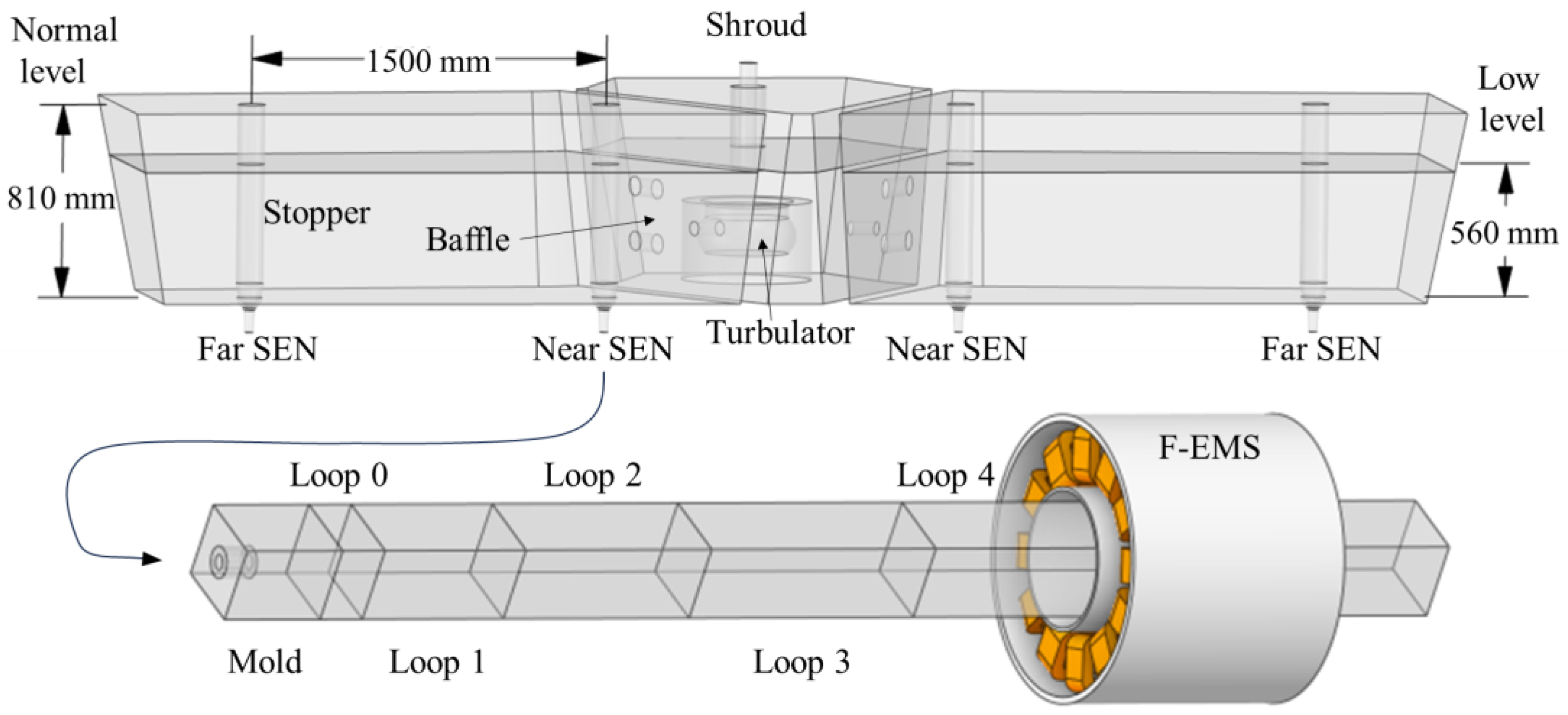
3.2.1. Tundish Simulation

Figure 4 depicts the variation in the mass fraction of the new grade over time during the steel grade transition in the tundish. The moment labeled as 0 in the chart corresponds to the time when the new grade starts flowing into the tundish from the ladle. Figure 4a represents the steel grade transition with GCr15 as the old grade and GCr15SiMn as the new grade at a low tundish level. In this case, the density of the old grade is greater than that of the new grade. Figure 4b illustrates the steel grade transition with 30Cr2Ni2Mo as the old grade and 30CrNi3Mo as the new grade at a low tundish level, where the density of the old grade is less than that of the new grade. Figure 4c represents the steel grade transition with Q345 as the old grade and Q355 as the new grade at a low tundish level, where the density of the old grade is approximately equal to that of the new grade.

It is evident from the figure that the steel grade transition in the tundish is significantly influenced by the density difference between the new and old grades. When the density of the old grade is greater than that of the new grade, the generation time of the mixed molten steel is shorter, resulting in fewer transition blooms. Conversely, when the density of the old grade is less than that of the new grade, the generation time of the mixed molten steel is longer, leading to more transition blooms.

Figure 4d illustrates the steel grade transition with GCr15 as the old grade and GCr15SiMn as the new grade at a normal tundish level. It can be observed that the greater the remaining amount of the old grade in the tundish, the longer the generation time of the mixed molten steel, and the more transition blooms are produced.

Figure 5a–d correspond to Figure 4a–d, respectively. In these figures, the black curve represents the dimensionless concentration history of the new grade at the far SEN (out 1), while the red curve represents the dimensionless concentration history of the new grade at the near SEN (out 2). The dimensionless concentration of the new grade at the SEN in the tundish model is converted into the mass fraction $C_{t,spe}$ of each solute element using Equation (1). This information is then compiled into a Profile file and imported at the entrance of the strand model for each element’s mass fraction. As the variation patterns in the bloom are similar, studying the steel grade transition of one strand is sufficient to understand the steel grade transition of the bloom. In this simulation, the strand from the near SEN (out 2) is chosen for further investigation.

3.2.2. F-EMS Simulation

Maxwell was employed to calculate the electromagnetic force and magnetic induction intensity generated by F-EMS for the bloom, as depicted in Figure 6. The electromagnetic force is imported into the strand model by compiling a user-defined function.

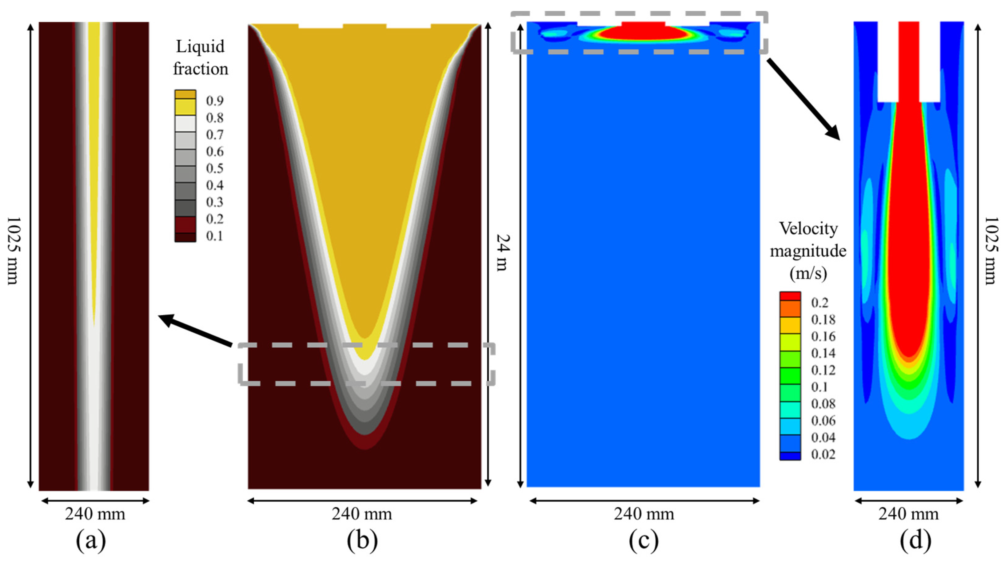
3.2.3. Old Grade Casting Simulation

From Figure 7b, it can be observed that the mushy zone has a large volume in the strand model, and solute elements continuously migrate from the solid phase through the mushy zone into the liquid phase. This results in significant differences in the mass fraction of the solute elements on the same cross-section of the bloom. Regarding the molten steel flow perspective shown in Figure 7c, the regions with a substantial difference between the molten steel flow velocity and the casting speed are mainly concentrated within 1 m below the meniscus. The impact of the molten steel flow on the mass fraction differences in the solute elements in the same cross-section of the bloom is relatively minor. In Figure 7b,c, the positions of the mushy zone and areas with a high molten steel flow velocity are compressed to show their locations in the complete bloom. On the other hand, Figure 7a,d are local magnifications of Figure 7b,c at normal proportions. Therefore, the macro-segregation of the solute elements has a much more significant impact on the mass fraction differences in the solute elements in the same cross-section of the bloom compared to the effect of the molten steel flow. When establishing a predictive model for the composition of the transition bloom, the influence of macro-segregation on the distribution of the solute elements cannot be ignored.

Numerical simulation of the continuous casting process with the old grade forms the foundation for simulating the steel grade transition. Figure 8 presents the numerical simulation results of the normal continuous casting process for the old grades GCr15, 30Cr2Ni2Mo, and Q345. Due to the actual aspect ratio of the computational domain being 100:1, the aspect ratio in the figure is reduced to 10:1 for better visualization of the simulation results. The following vertical section contour maps use this compression ratio. Figure 8a,c,e, respectively, show the liquid fraction contour maps for the old grades GCr15, 30Cr2Ni2Mo, and Q345. Due to the composition differences between the three steel grades leading to different solidus and liquidus temperatures, they eventually result in different solidification endpoints. The elements with the greatest differences in each steel grade transition scheme are then displayed in Figure 8b,d,f. Among them, Figure 8b illustrates the distribution of the Si element in GCr15, Figure 8d shows the distribution of the Ni element in 30Cr2Ni2Mo, and Figure 8f displays the distribution of the Mn element in Q345. During the solidification process of the bloom, a liquid phase, a solid phase, and a mushy zone in between exist. The solute elements undergo redistribution at the solidification front, which is the primary cause of macro-segregation in the bloom. Before the solidification is completed, there is a relatively long mushy zone that accumulates the high-concentration solute elements expelled by the surrounding bloom. This leads to significant positive macro-segregation in the center of the bloom, increasing the compositional differences in the bloom’s cross-section.

The differences in the thermal physical parameters of the solute elements result in them having different segregation degrees. There are various methods for defining the segregation degree, and Wołczyński’s [38] method can be used to observe the distribution of solute elements throughout the cross-section. This article uses Equation (25) to calculate the segregation degree $r_{spe}$ for each element.

$$r_{spe}=\frac{C_{spe}}{{\overline{c}}_{spe}}$$

(25)

where ${\overline{c}}_{spe}$ represents the average mass fraction of the element ${spe}^{th}$. The segregation degrees of various elements in the cross-section of the fully solidified blooms for the old grades GCr15, 30Cr2Ni2Mo, and Q345 are shown in Figure 9. From Figure 9a, the order of the center segregation of the elements is C > Si > Mn > Cr. In Figure 9b, the order of the center segregation of the elements is Mo > Mn > Cr > Ni. Figure 9c reveals that the order of the center segregation of the elements is C > Si = Mn. It can be observed that the segregation degree of the elements is closely related to the distribution coefficients of each element in different phases.

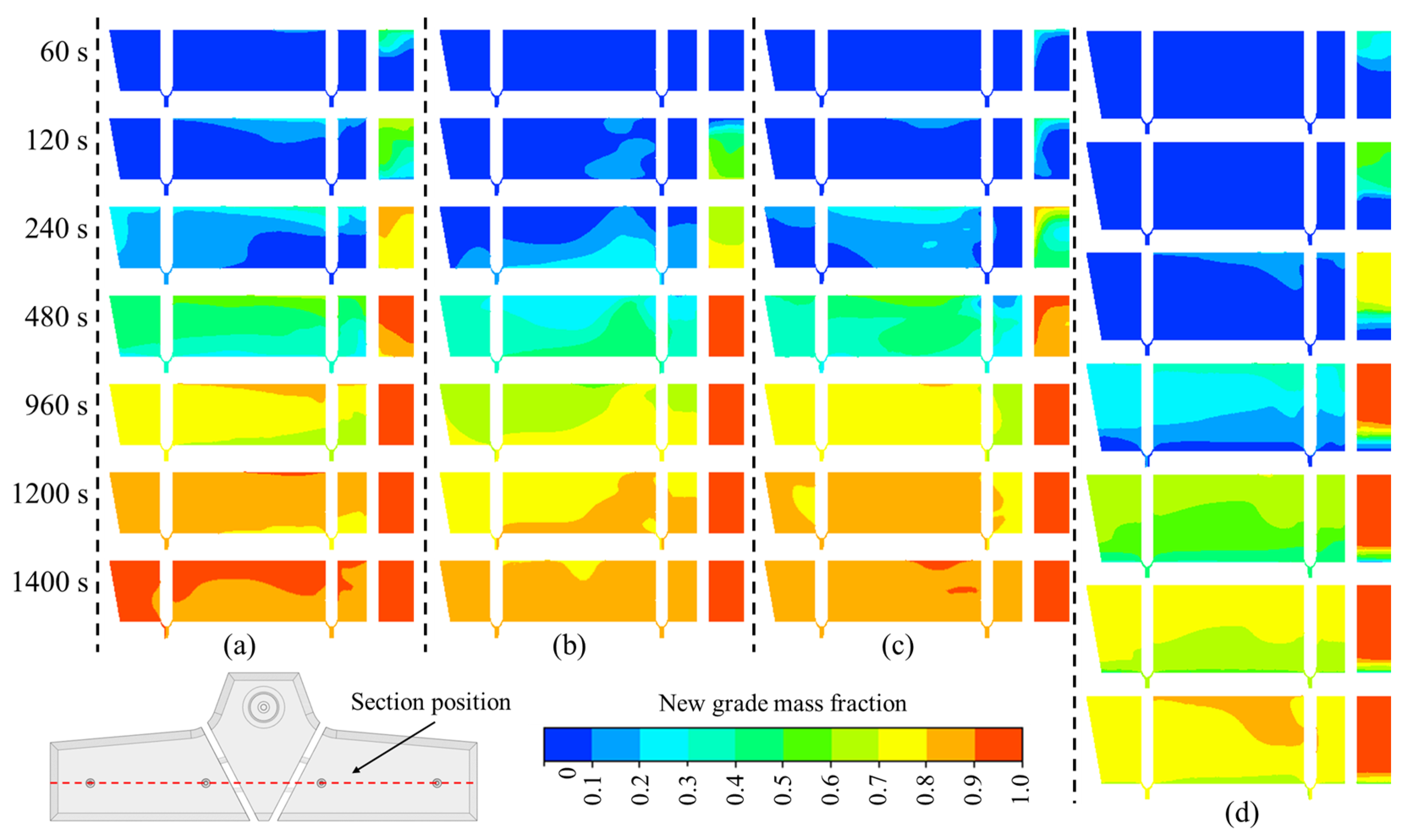
3.3. Formation Process of Transition Blooms with Different Carbon Contents

After the molten steel enters the mold, it flows downward along the solidification front under the influence of the flow field. At the initial stage of the steel grade transition, the center of the same cross-section of the bloom is the old grade, and the solidification front of the bloom is the new grade. As the bloom further solidifies, the effect of macro-segregation becomes evident. The solute element mass fraction at the center of the bloom cross-section gradually becomes higher than that of the new grade at the solidification front, becoming the defining condition for the starting point of the transition bloom.

Figure 10a–c, respectively, illustrate the steel grade transition of the old grade GCr15 and new grade GCr15SiMn, the old grade 30Cr2Ni2Mo and new grade 30CrNi3Mo, and the old grade Q345 and new grade Q355. When GCr15 is the old grade and GCr15SiMn is the new grade, the equilibrium distribution coefficient of the Si element in the austenite phase is relatively small, leading to a higher segregation degree. Therefore, in Scheme 1, there is a significant difference in the mass fraction of the Si element in the same cross-section. When 30Cr2Ni2Mo is the old grade and 30CrNi3Mo is the new grade, the equilibrium distribution coefficients of the Ni element in both the austenite phase and the ferrite phase are relatively large, resulting in a smaller segregation degree. Therefore, in Scheme 2, there is a smaller difference in the mass fraction of the Ni element in the same cross-section. When Q345 is the old grade and Q355 is the new grade, the equilibrium distribution coefficients of the Mn element in the ferrite phase are relatively large, resulting in a smaller segregation degree. Therefore, in Scheme 3, there is a smaller difference in the mass fraction of the Mn element in the same cross-section. However, in Scheme 3, the difference in the mass fraction of the Mn element between the new and old grades is also relatively small, leading to a larger difference after converting the Mn element into a dimensionless concentration.

Figure 11 shows the dimensionless concentration history of the average mass fraction of the new grade at the exit of the tundish, as well as the curve drawn from the center segregation value, average value, and sub-surface negative segregation value of the transition bloom. Figure 11a depicts the history of the Si element mass fraction of the transition bloom when GCr15 is the old grade and GCr15SiMn is the new grade in the steel grade transition. In this scheme, the Si element mass fractions of the new and old grades differ significantly, and the actual composition of the Si element of both steel grades is far from the control line (y = 0.35 and y = 0.40) of the steel grade composition range. The previous transition bloom prediction method did not consider the macro-segregation phenomenon in the transition bloom. The original method determined a relatively short transition bloom of 8.88 m. The new scheme, considering the macro-segregation in the transition bloom, calculates a longer transition bloom of 10.88 m compared to the original scheme. Figure 11b shows the history of the Ni element mass fraction of the transition bloom when 30Cr2Ni2Mo is the old grade and 30CrNi3Mo is the new grade in the steel grade transition. In this scheme, the Ni element mass fractions of the new and old grades differ significantly, and the actual composition of the Ni element of both steel grades is close to the control line (y = 2.20 and y = 2.75) of the steel grade composition range. The original method determined a relatively long transition bloom of 34.64 m. The new scheme calculates a slightly longer transition bloom of 35.16 m compared to the original scheme. Figure 11c illustrates the history of the Mn element mass fraction of the transition bloom when Q345 is the old grade and Q355 is the new grade in the steel grade transition. In this scheme, the Mn element mass fractions of the new and old grades overlap, and the original method considered no transition bloom, with a determined division interval of 4.08 m. The new scheme calculates a shorter division interval for the new and old grades, only 0.94 m compared to the original scheme.

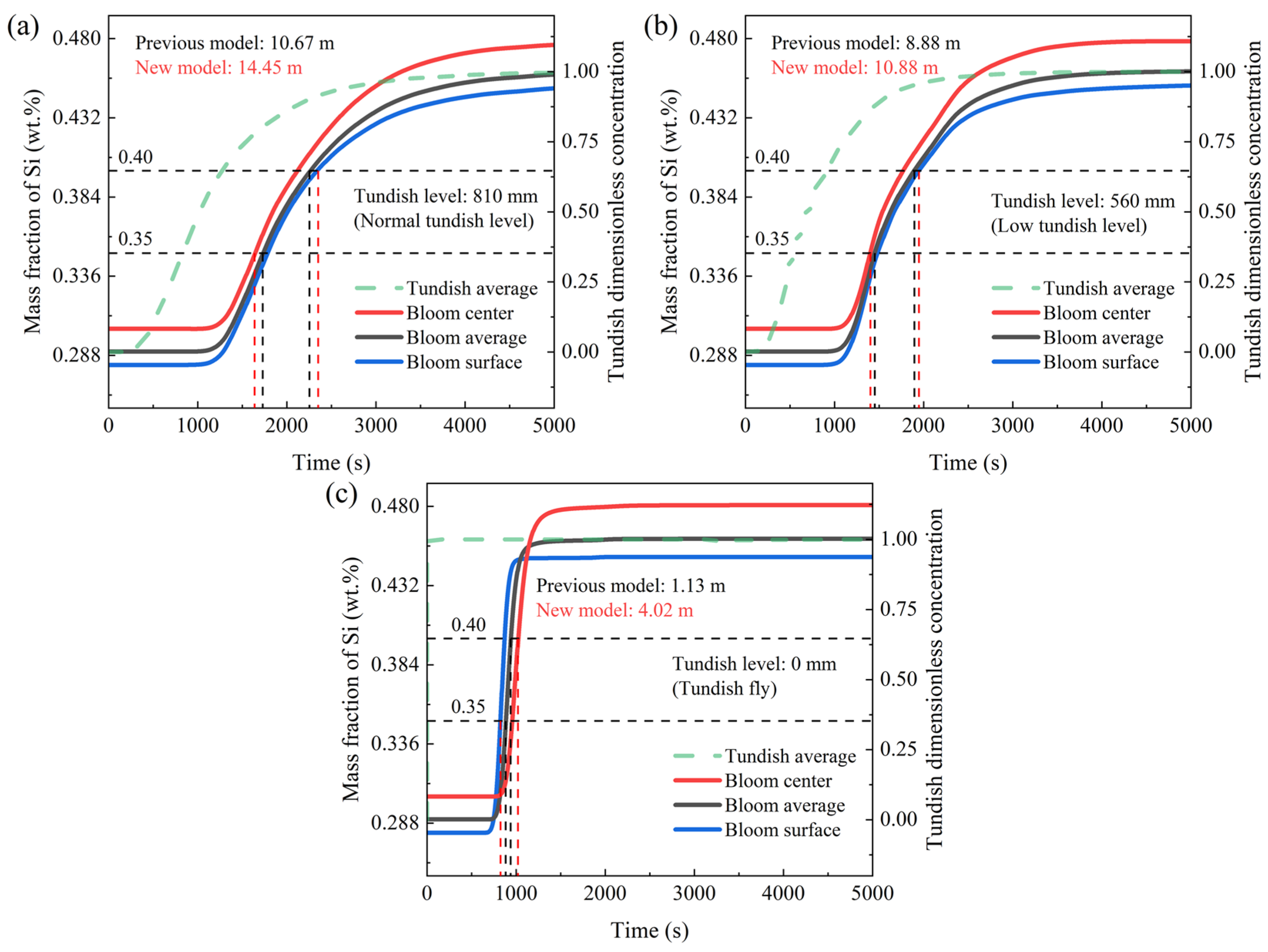
3.4. Different Tundish Levels in Steel Grade Transition

This study investigates the steel grade transition with different tundish levels using GCr15 as the old grade and GCr15SiMn as the new grade, as illustrated in Figure 12. Figure 12a depicts the steel grade transition under a normal tundish level, while Figure 12b shows the steel grade transition with the minimum tundish level, and Figure 12c illustrates the steel grade transition with a flying tundish. When there is an overlap in the compositions of the old and new grades, it is recommended to use the normal tundish level to obtain a longer separation interval between the old and new grades. In cases where there is a significant difference in the composition between the old and new grades during the steel grade transition, the use of the minimum tundish level, which does not cause tundish powder entrainment, or the flying tundish method is advised. Figure 12c demonstrates the flying tundish technique without the simultaneous use of a “grade separator”. It is evident that, influenced by the flow field and macro-segregation, there is a substantial difference in the mass fraction of the solute elements across the same transverse section of the transition bloom, resulting in a longer transition bloom. Therefore, when employing the flying tundish method, it is recommended to use a grade separator concurrently to effectively reduce the uneven distribution of the solute elements across the same transverse section caused by the flow field [6].

Figure 13 illustrates the dimensionless concentration history by plotting the average mass fraction of the new steel at the tundish outlet, along with the RTD curve plotted based on the center segregation value, average value, and subcutaneous negative segregation value of the transition bloom. Figure 13a depicts the historical concentration of the Si element for the steel grade transition with a normal tundish level. The original method determined a length of 10.67 m for the transition blooms. The new approach calculates a length of 14.45 m for the transition blooms, longer than the original method. Figure 13b presents the historical concentration of the Ni element for the steel grade transition with the lowest tundish level. The original method determined a transition bloom length of 8.88 m. The new approach calculates a transition bloom length of 10.88 m, longer than the original method. Figure 13c shows the historical concentration of the Mn element for the steel grade transition with a flying tundish. The original method determined a transition bloom length of 1.13 m. The new approach calculates a transition bloom length of 4.02 m, longer than the original method.

The initiation of the sub-surface negative segregation (blue) curves in Figure 13a–c occurs earlier than that of the average composition (black) curves, and the average composition curve change occurs earlier than that of the central segregation (red) curves at the initiation stage. For Figure 13a,b, the composition changes in the mixed molten steel are relatively slow. When the sub-surface negative segregation (blue) curves rise to the position of the average composition (black) curves, the average composition (black) curves have also risen, and the two curves do not intersect. Similarly, the average composition (black) curves and the central segregation (red) curves do not intersect either. Therefore, the control curve for the initial division position is the central segregation (red) curve, and for the final division position, it is the sub-surface negative segregation (blue) curve.

However, the composition changes in the mixed molten steel in Figure 13c occur too rapidly. When the sub-surface negative segregation (blue) curve rises to the position of the average composition (black) curve, the average composition (black) curve has not yet risen, resulting in the intersection of the two curves. Similarly, the average composition (black) curve intersects with the central segregation (red) curve, and the sub-surface negative segregation (blue) curve also intersects with the central segregation (red) curve. This leads to the control curve for the initial division position being the sub-surface negative segregation (blue) curve, and for the final division position, it is the central segregation (red) curve.

4. Conclusions

This study established a comprehensive numerical model for the entire process of steel grade transition, from the ladle shroud of the tundish to the solidification endpoint of the bloom. The model incorporates physical phenomena such as fluid flow, an electromagnetic field, heat transfer, solidification, and solute transport. The accuracy of the numerical simulation was validated by comparing the measured and simulated values of the Si element mass fraction in the transition bloom, where GCr15 serves as the old steel and GCr15SiMn serves as the new steel. The main findings of this study are summarized as follows:

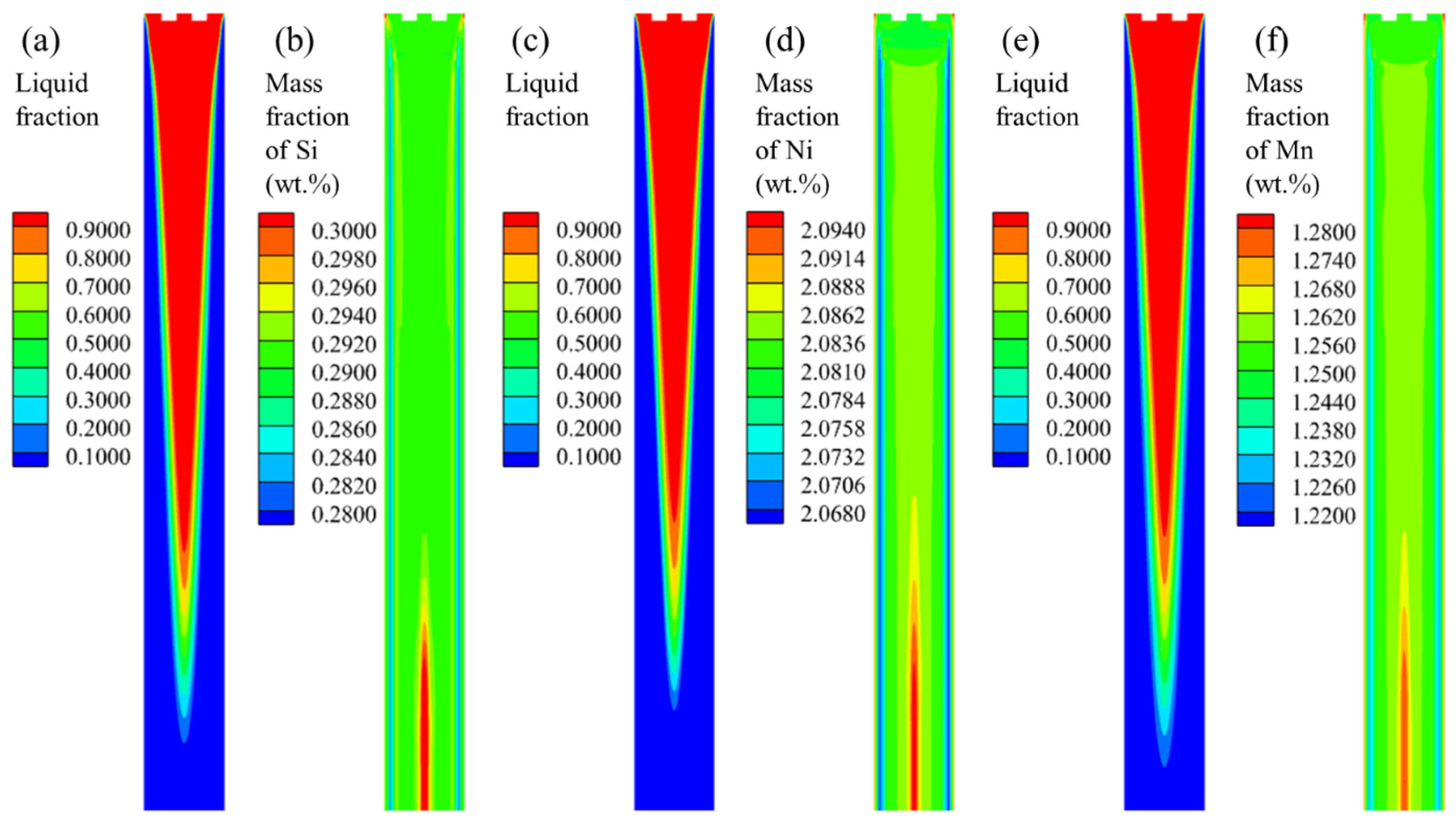
• The regions where the difference between the molten steel velocity and the casting speed is significant are mainly concentrated within 1 m below the meniscus. The influence of the molten steel flow on the mass fraction difference in the solute elements in the same cross-section of the transition bloom is relatively small. The voluminous mushy zone in the strand model leads to the continuous migration of solute elements from the solid phase through the mushy zone into the liquid phase. This results in macro-segregation, where the impact of macro-segregation on the mass fraction difference in the solute elements in the same cross-section of the transition bloom is much greater than that of the molten steel flow.
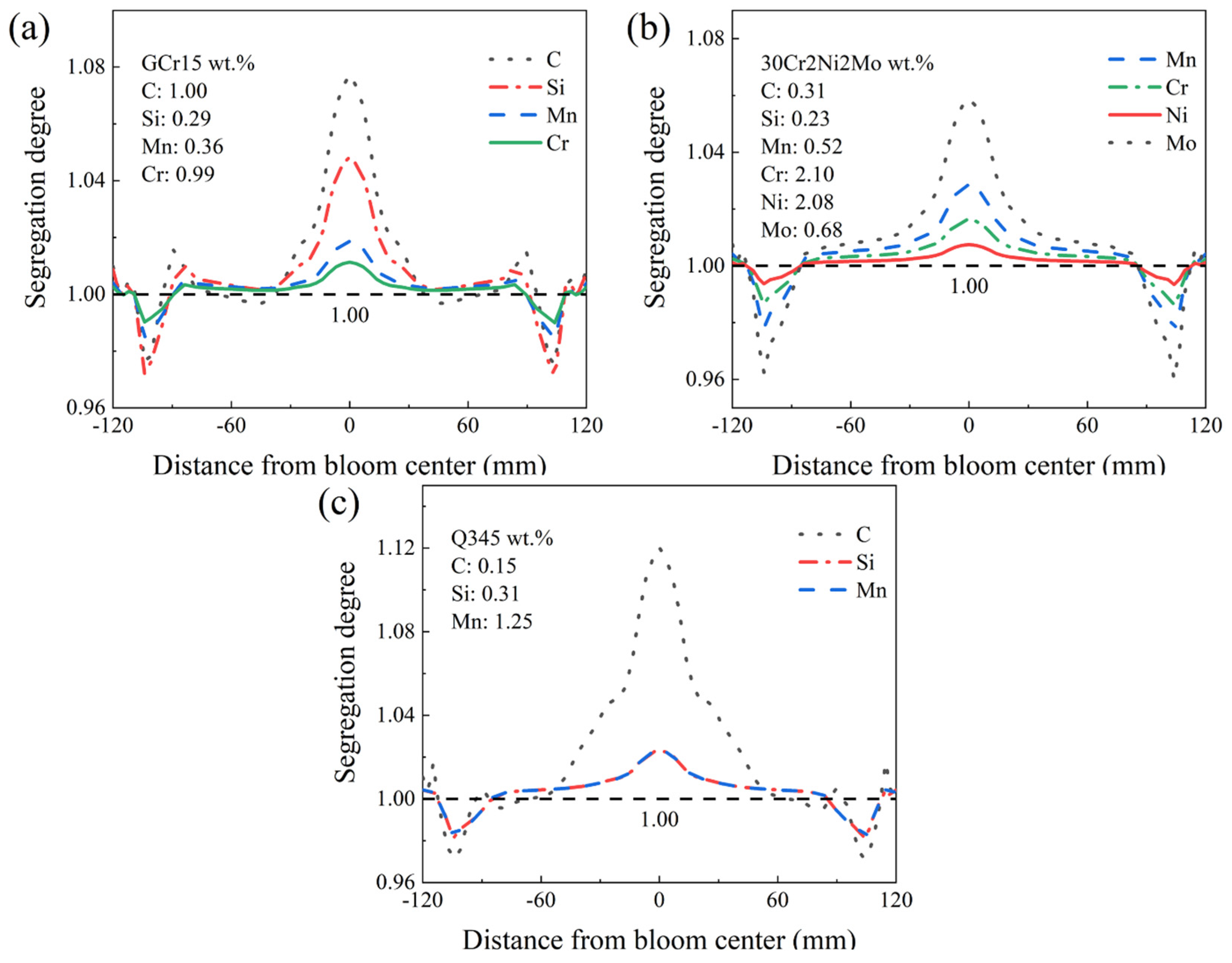
• The steel grade transition process for various solute elements in different phases exhibits similarities. The segregation degrees of the solute elements are closely related to their distribution coefficients in different phases. The segregation degree order of the solute elements in the austenite phase is as follows: C > Si > Mo > Mn > Cr > Ni. In the ferrite phase, it is C > Si = Mn.
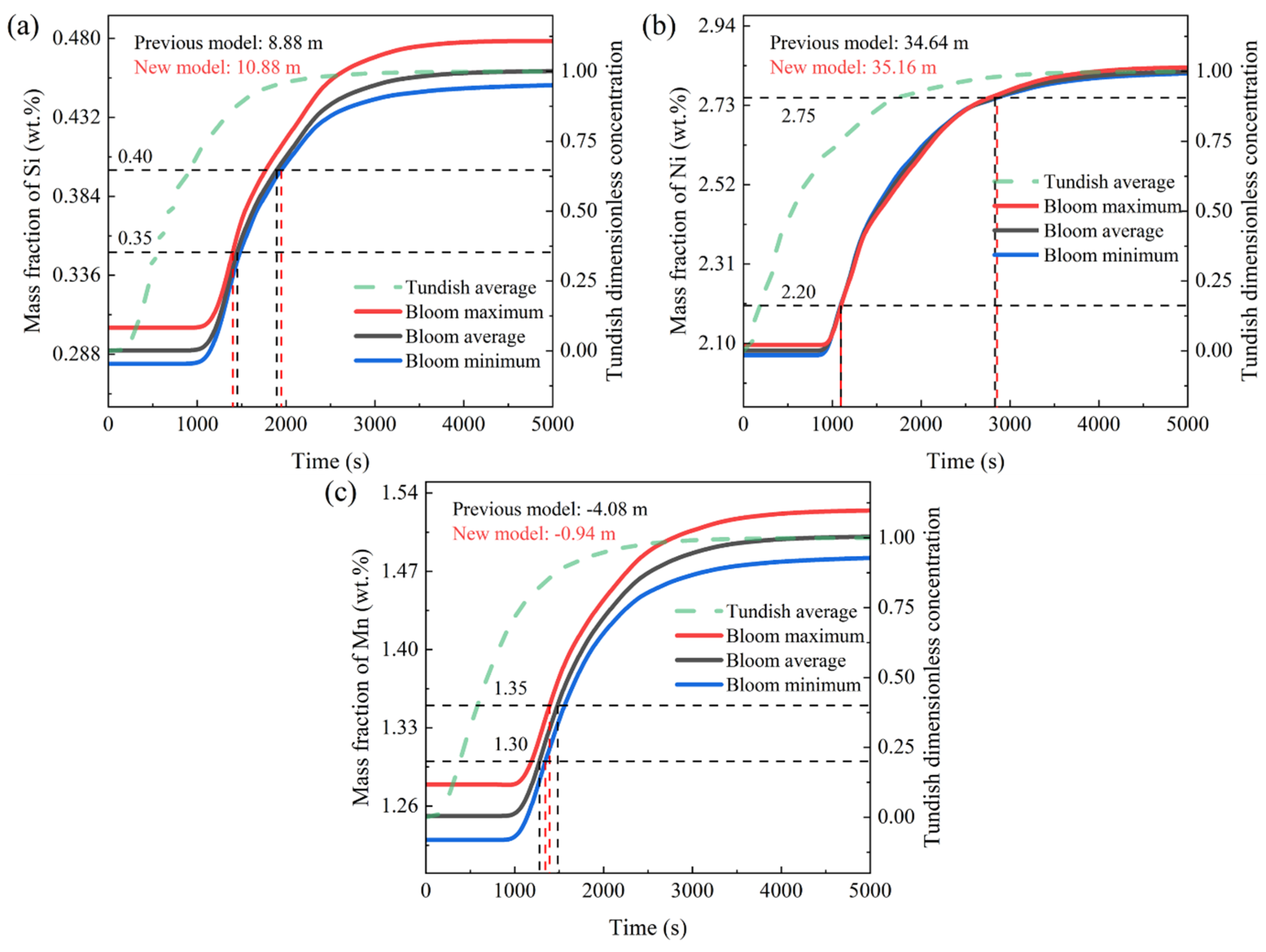
• The transition bloom division model considering macro-segregation is more rigorous than the original division method. This results in longer transition blooms when there is significant dissimilarity between the old and new grades. For example, in Scheme 1, the original division method determines a transition bloom length of 8.88 m, while the new method calculates a length of 10.88 m. In Scheme 2, the original division method gives a transition bloom length of 34.64 m, while the new method calculates a length of 35.16 m. Simultaneously, it also leads to a shorter partition interval when there is an overlap in the composition of the old and new grades. For example, in Scheme 3, the original method determines a partition interval of 4.08 m, while the new method calculates a length of 0.94 m.
• When there is an overlap in the composition of the old and new grades, it is recommended to use the normal tundish level, which can slow down the mixing of the old and new grades, allowing for a longer partition interval. When there is a significant difference in the composition of the old and new grades in the steel grade transition, it is recommended to use the minimum tundish level, which does not cause tundish powder entrapment, or to use the flying tundish method. Increasing the rate of change in the composition of the old and new grades shortens the length of the transition bloom. When using the flying tundish method, it should be combined with the use of a “grade separator” to effectively reduce the uneven distribution of the solute elements in the same cross-section of the transition bloom caused by the flow field. At the same time, attention should be paid to the actual composition of the solute elements, especially in the new steel, which differ significantly in their mass fractions, and should be kept away from the control lines of the steel composition ranges.

References

1. Siddiqui, M.I.H.; Kim, M.H. Optimization of flow control devices to minimize the grade mixing in steelmaking tundish. Iran. J. Sci. Technol. 2018, 32, 3213–3221. [Google Scholar] [CrossRef]
2. Kumar, R.; Siddiqui, M.I.H.; Jha, P.K. Numerical investigations on the use of flow modifiers in multi-strand continuous casting tundish using RTD curves analysis. In Proceedings of the International Conference on Smart Technologies for Mechanical Engineering, Delhi, India, 25–26 October 2013; pp. 603–612. [Google Scholar]
3. Siddiqui, M.I.H.; Jha, P.K. Effect of inflow rate variation on intermixing in a steelmaking tundish during ladle change-over. Steel Res. Int. 2016, 87, 733–744. [Google Scholar] [CrossRef]
4. Agarwal, R.; Singh, M.K.; Kumar, R.B.; Ghosh, B.; Pathak, S. Extensive analysis of multi strand billet caster tundish using numerical technique. World J. Mech. 2019, 9, 29–51. [Google Scholar] [CrossRef]
5. Michalek, K.; Gryc, K.; Tkadleková, M.; Morávka, J.; Huczala, T.; Bocek, D.; Horáková, D. Type of submerged entry nozzle vs. concentration profiles in the intermixed zone of round blooms with a diameter of 525 mm. Mater. Technol. 2012, 46, 581–587. [Google Scholar]
6. Huang, X.; Thomas, B.G. Intermixing model of continuous casting during a grade transition. Metall. Mater. Trans. B 1996, 27, 617–632. [Google Scholar] [CrossRef]
7. Thomas, B.G. Modeling study of intermixing in tundish and strand during a continuous-casting grade transition. Iron Steelmak. 1997, 24, 83–96. [Google Scholar]
8. Thomas, B.G. The importance of computational models for further improvements of the continuous casting process. In Proceedings of the Voest Alpine Conference on Continuous Casting, Linz, Austria, 5–7 June 2000. [Google Scholar]
9. Rappaz, M. Modelling of microstructure formation in solidification processes. Int. Mater. Rev. 1989, 34, 93–124. [Google Scholar] [CrossRef]
10. Rappaz, M.; Gandin, C.A.; Desbiolles, J.L.; Thévoz, P. Prediction of grain structures in various solidification processes. Metall. Mater. Trans. A 1996, 27, 695–705. [Google Scholar] [CrossRef]
11. Campanella, T.; Charbon, C.; Rappaz, M. Grain refinement induced by electromagnetic stirring: A dendrite fragmentation criterion. Metall. Mater. Trans. A 2004, 35, 3201–3210. [Google Scholar] [CrossRef]
12. Chen, C.; Cheng, G. Delta-ferrite distribution in a continuous casting slab of Fe-Cr-Mn austenitic stainless steel. Metall. Mater. Trans. B 2017, 48, 2324–2333. [Google Scholar] [CrossRef]
13. Dong, Q.; Zhang, J.; Yin, Y.; Nagaumi, H. Numerical simulation of macrosegregation in billet continuous casting influenced by electromagnetic stirring. J. Iron Steel Res. Int. 2022, 29, 612–627. [Google Scholar] [CrossRef]
14. Chen, H.; Long, M.; Chen, D.; Liu, T.; Duan, H. Numerical study on the characteristics of solute distribution and the formation of centerline segregation in continuous casting (CC) slab. Int. J. Heat Mass Transfer 2018, 126, 843–853. [Google Scholar] [CrossRef]
15. Li, S.; Han, Z.; Zhang, J. Numerical modeling of the macrosegregation improvement in continuous casting blooms by using F-EMS. JOM 2020, 72, 4117–4126. [Google Scholar] [CrossRef]
16. Hou, Z.; Cheng, G.; Wu, C.; Chen, C. Time-series analysis technologies applied to the study of carbon element distribution along casting direction in continuous-casting billet. Metall. Mater. Trans. B 2012, 43, 1517–1529. [Google Scholar] [CrossRef]
17. Szmyd, J.S.; Suzuki, K. Modelling of Transport Phenomena in Crystal Growth; WIT Press: Southampton, UK, 2000. [Google Scholar]
18. Huang, X.; Thomas, B.G. Modeling of steel grade transition in continuous slab casting processes. Metall. Mater. Trans. B 1993, 24, 379–393. [Google Scholar] [CrossRef]
19. Wang, Q.; Tan, C.; Huang, A.; Yan, W.; Gu, H.; He, Z.; Li, G. Numerical simulation on refractory wear and inclusion formation in continuous casting tundish. Metall. Mater. Trans. B 2021, 52, 1344–1356. [Google Scholar] [CrossRef]
20. Li, Q.; Qin, B.; Zhang, J.; Dong, H.; Li, M.; Tao, B.; Mao, X.; Liu, Q. Design Improvement of Four-Strand Continuous-Casting Tundish Using Physical and Numerical Simulation. Materials 2023, 16, 849–863. [Google Scholar] [CrossRef] [PubMed]
21. Yi, B.; Zhang, G.; Jiang, Q.; Zhang, P.; Feng, Z.; Tian, N. The Removal of Inclusions with Different Diameters in Tundish by Channel Induction Heating: A Numerical Simulation Study. Materials 2023, 16, 5254–5266. [Google Scholar] [CrossRef]
22. Chen, H.; Liu, Z.; Li, F.; Lyu, B.; Chen, W.; Zhang, L. Numerical Simulation on Multiphase Flow and Slag Entrainment during Casting Start of a Slab Continuous Casting Tundish. Metall. Mater. Trans. B 2023, 54, 2048–2065. [Google Scholar] [CrossRef]
23. Figueroa-Fierros, A.E.; Ramos-Banderas, J.Á.; Hernández-Bocanegra, C.A.; López-Granados, N.M.; Solorio-Díaz, G. Thermal-Fluid Dynamic Behavior on Intermixed Steel Calculation during a Grade Change in a Slab Tundish by Numerical Simulation. ISIJ Int. 2023, 63, 1998–2009. [Google Scholar] [CrossRef]
24. Pieprzyca, J.; Merder, T.; Saternus, M.; Tkadlecková, M.; Cupek, J.; Walek, J. Modeling research on limitation of transition zone during continuous steel casting. Metalurgija 2024, 63, 3–5. [Google Scholar]
25. Jeon, S.; Lee, S.; Ha, S.; Kim, S.; You, D. Effects of a moving weir on tundish flow during continuous-casting grade-transition. J. Mech. Sci. Technol. 2021, 35, 4001–4009. [Google Scholar] [CrossRef]
26. Yin, S.; Luo, S.; Zhang, W.; Wang, W.; Zhu, M. Numerical simulation of macrosegregation in continuously cast gear steel 20CrMnTi with final electromagnetic stirring. J. Iron Steel Res. Int. 2021, 28, 424–436. [Google Scholar] [CrossRef]
27. Wu, H.; Xu, C.; Lei, C.; Wang, T.; Gao, Y.; Zhang, X.; Jin, H. Numerical Simulation and Industrial Experiment of the Fluid Flow and Heat Transfer in Large Vertical Round Billets with Helical Final Electromagnetic Stirring. JOM 2023, 75, 1439–1449. [Google Scholar] [CrossRef]
28. Liu, H.; Chen, Y.; Qiu, H.; Wang, Z. Numerical simulation of coupled fluid flow and solidification in a curved round bloom continuous caster with a combined rotary electromagnetic stirring. Ironmak. Steelmak. 2022, 49, 506–521. [Google Scholar] [CrossRef]
29. Guan, R.; Ji, C.; Zhu, M. Modeling the effect of combined electromagnetic stirring modes on macrosegregation in continuous casting blooms. Metall. Mater. Trans. B 2020, 51, 1137–1153. [Google Scholar] [CrossRef]
30. Tan, R.; Liu, W.; Song, B.; Yang, S.; Chen, Y.; Zuo, X.; Huang, Y. Numerical simulation on solidification behavior and structure of 38CrMoAl large round bloom using CAFE model. J. Iron Steel Res. Int. 2023, 30, 1222–1233. [Google Scholar] [CrossRef]
31. Song, S.; Sun, Y.; Li, Y.; Zhuo, C. Effects of Temperature and Density on Transition Slab Length during Steel Grade Transition. In Proceedings of the TMS Annual Meeting & Exhibition, San Diego, CA, USA, 19–23 March 2023; pp. 227–240. [Google Scholar]
32. Li, S. Numerical Study on the Macroscopic Transport Phenomena of Continuous Casting Process under Electromagnetic Force. Ph.D. Thesis, University of Science and Technology Beijing, Beijing, China, 2020. [Google Scholar]
33. Launder, B.E.; Spalding, D.B. Lectures in Mathematical Models of Turbulence; Academic Press: Cambridge, MA, USA, 1972. [Google Scholar]
34. Zhong, H.; Wang, R.; Han, Q.; Fang, M.; Yuan, H.; Song, L.; Xie, X.; Zhai, Q. Solidification structure and central segregation of 6Cr13Mo stainless steel under simulated continuous casting conditions. J. Mater. Res. Technol. 2022, 20, 3408–3419. [Google Scholar] [CrossRef]
35. Song, S.; Sun, Y.; An, H. Numerical modeling of grade mixing and inclusion entrapment in eight strand billet tundish. Metall. Res. Technol. 2023, 120, 1–15. [Google Scholar] [CrossRef]
36. Meng, Y.A.; Thomas, B.G. Heat-transfer and solidification model of continuous slab casting: CON1D. Metall. Mater. Trans. B 2003, 34, 685–705. [Google Scholar] [CrossRef]
37. Schneider, M.C.; Beckermann, C. Simulation of micro-/macrosegregation during the solidification of a low-alloy steel. ISIJ Int. 1995, 35, 665–672. [Google Scholar] [CrossRef]
38. Wołczyński, W. Nature of segregation in the steel static and brass continuously cast ingots. Arch. Metall. Mater. 2018, 63, 1915–1922. [Google Scholar] [CrossRef]
Figure 1. Schematic diagram of a 3D geometric.
Metals 14 00263 g001
Figure 2. A schematic diagram of the crystallization process of three pairs of steel grades in steel grade transition.
Metals 14 00263 g002
Figure 3. Simulated and measured values of Si content in transition bloom of Scheme 1.
Metals 14 00263 g003
Figure 4. Contour maps of the change in mass fraction of new grades in the tundish over time during the steel grade transition: (a) Scheme 1; (b) Scheme 2; (c) Scheme 3; (d) Scheme 4.
Metals 14 00263 g004
Figure 5. Residence time distribution (RTD) curve of the mass fraction of new grades at each SEN of the tundish during the steel grade transition: (a) Scheme 1; (b) Scheme 2; (c) Scheme 3; (d) Scheme 4.
Metals 14 00263 g005
Figure 6. Electromagnetic force and magnetic induction intensity calculated using Maxwell: (a) F-EMS center cross-section electromagnetic force distribution; (b) magnetic induction intensity at the centerline of the bloom.
Metals 14 00263 g006
Figure 7. Comparison between the mushy zone and the area with significant differences in molten steel flow velocity: (a) local mushy zone at the solidification end; (b) the overall mushy zone in the continuous casting process of bloom; (c) the overall flow field in the continuous casting process of bloom; (d) local flow field in the mold.
Metals 14 00263 g007
Figure 8. Solidification and segregation during continuous casting of three old grades: (a) solidification of GCr15; (b) Si element segregation in GCr15; (c) solidification of 30Cr2Ni2Mo; (d) Ni element segregation in 30Cr2Ni2Mo; (e) solidification of Q345; (f) Mn element segregation in Q345.
Metals 14 00263 g008
Figure 9. The segregation degree of each solute element after solidification of three old grades: (a) GCr15; (b) 30Cr2Ni2Mo; (c) Q345.
Metals 14 00263 g009
Figure 10. Contour maps of the most influential elements over time in the strand model of the steel grade transition with different C content schemes: (a) the variation in Si element over time in Scheme 1; (b) the variation in Ni element over time in Scheme 2; (c) the variation in Mn element over time in Scheme 3.
Metals 14 00263 g010
Figure 11. RTD curves of the most influential elements over time in the strand model of the steel grade transition with different C content schemes: (a) the variation in Si element over time in Scheme 1; (b) the variation in Ni element over time in Scheme 2; (c) the variation in Mn element over time in Scheme 3.
Metals 14 00263 g011
Figure 12. Contour maps of Si element variation over time for a steel grade transition strand model with GCr15 as the old grade and GCr15SiMn as the new grade under different tundish level schemes: (a) the tundish level is 810 mm; (b) the tundish level is 560 mm; (c) the tundish level is 0 mm.
Metals 14 00263 g012
Figure 13. RTD curves of Si element variation over time for a steel grade transition strand model with GCr15 as the old grade and GCr15SiMn as the new grade under different tundish level schemes: (a) the tundish level is 810 mm; (b) the tundish level is 560 mm; (c) the tundish level is 0 mm.
Metals 14 00263 g013