
A Physically Motivated Heat Source Model for Laser Beam Welding

 , , and
Abstract
:1. Introduction
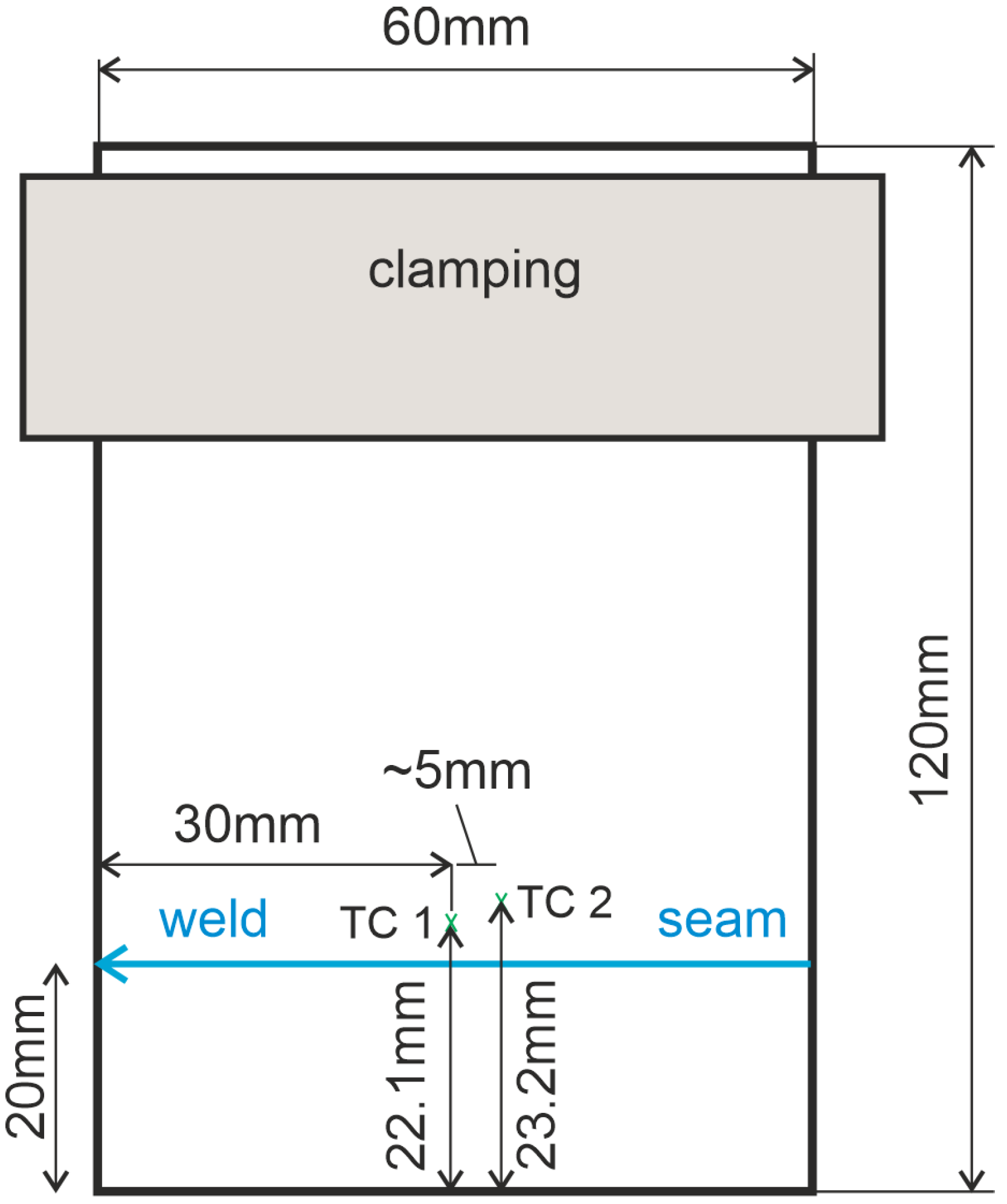
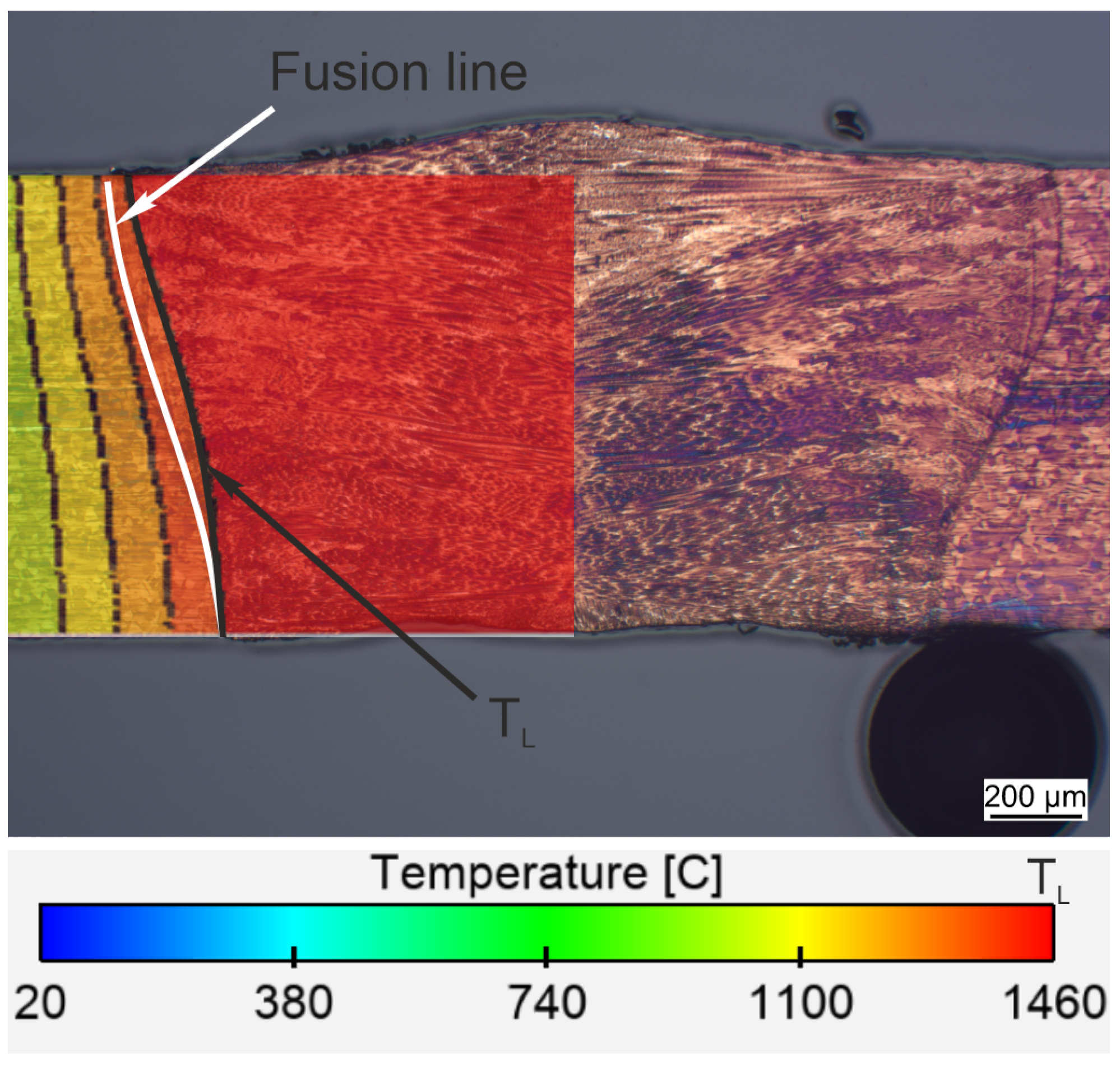
2. Experiments
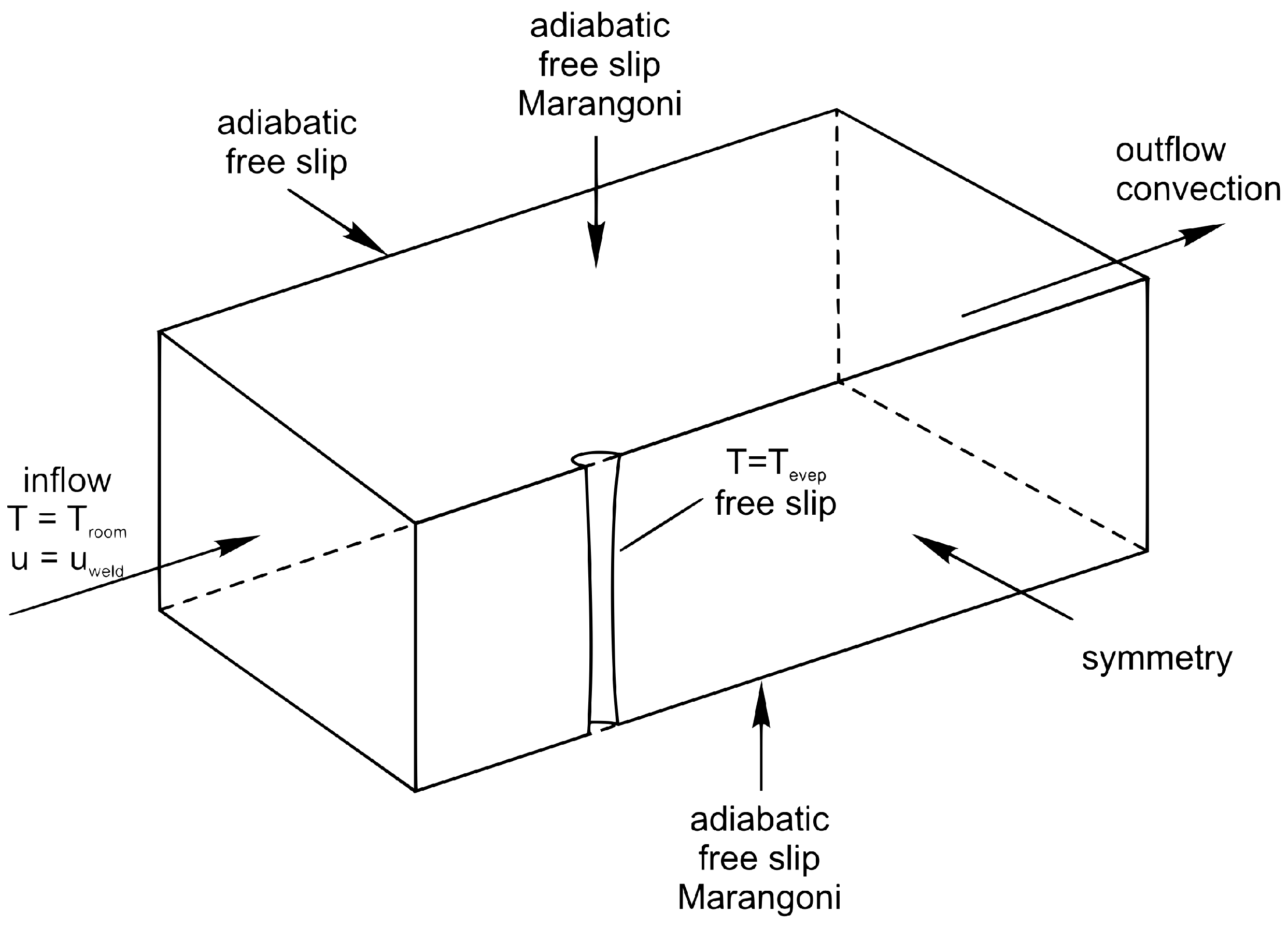
3. CFD Simulation and Material Parameters
- Steady-state approach;
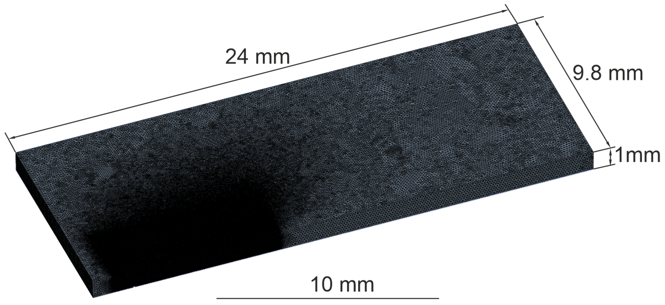
- Adapted size of the computational domain;
- Fixed free surface geometry;
- Approximated simplified and fixed keyhole geometry;
- Shear stress due to the interaction of metal vapor and liquid metal was not considered;
- Heat losses by radiation were neglected due to the high relation of the volume versus the surface of the plate.
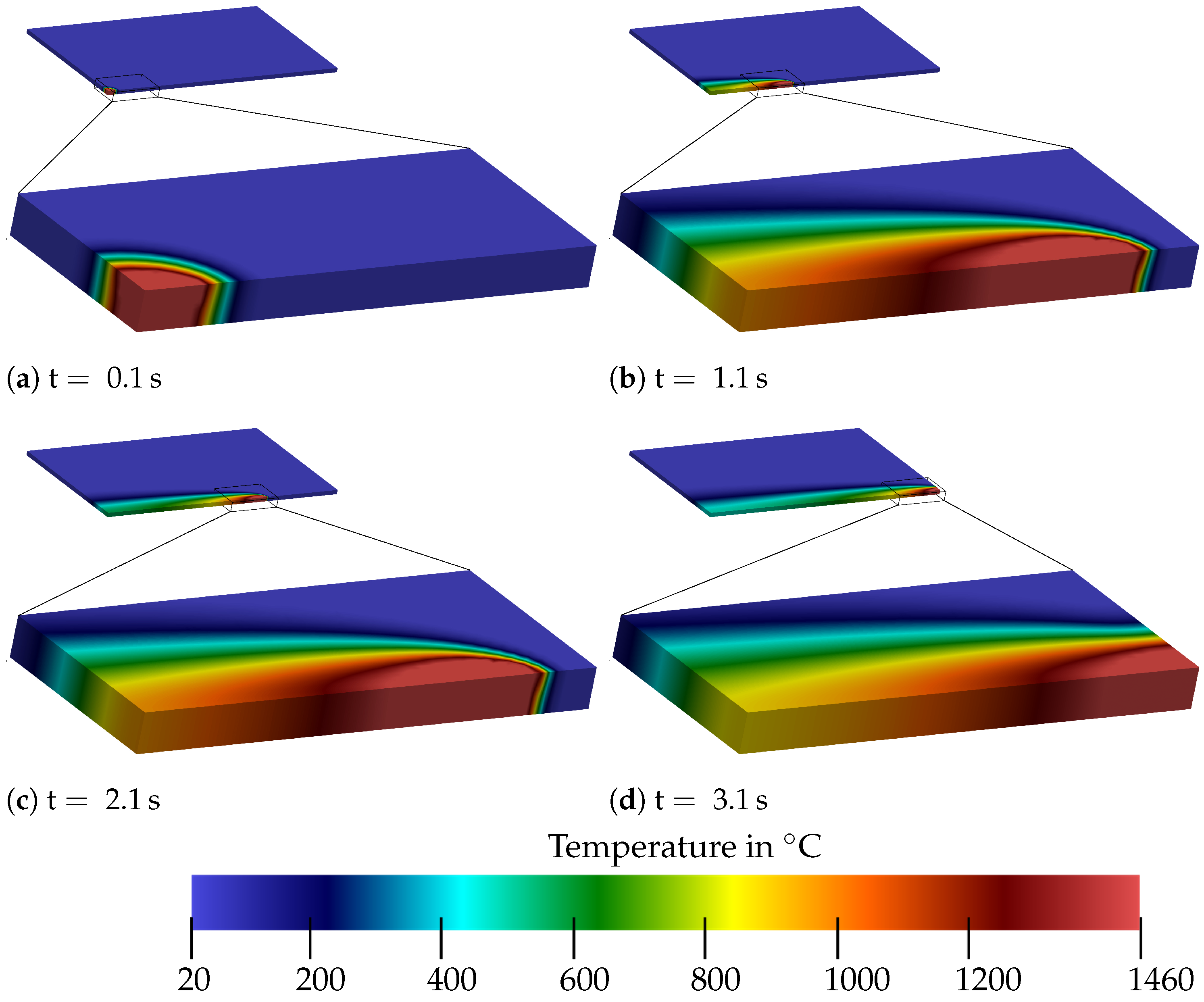
CFD Results
4. A Physically Motivated Heat Source Model
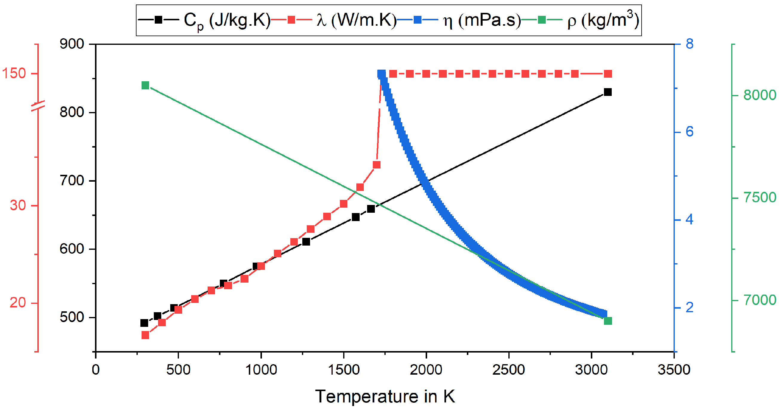
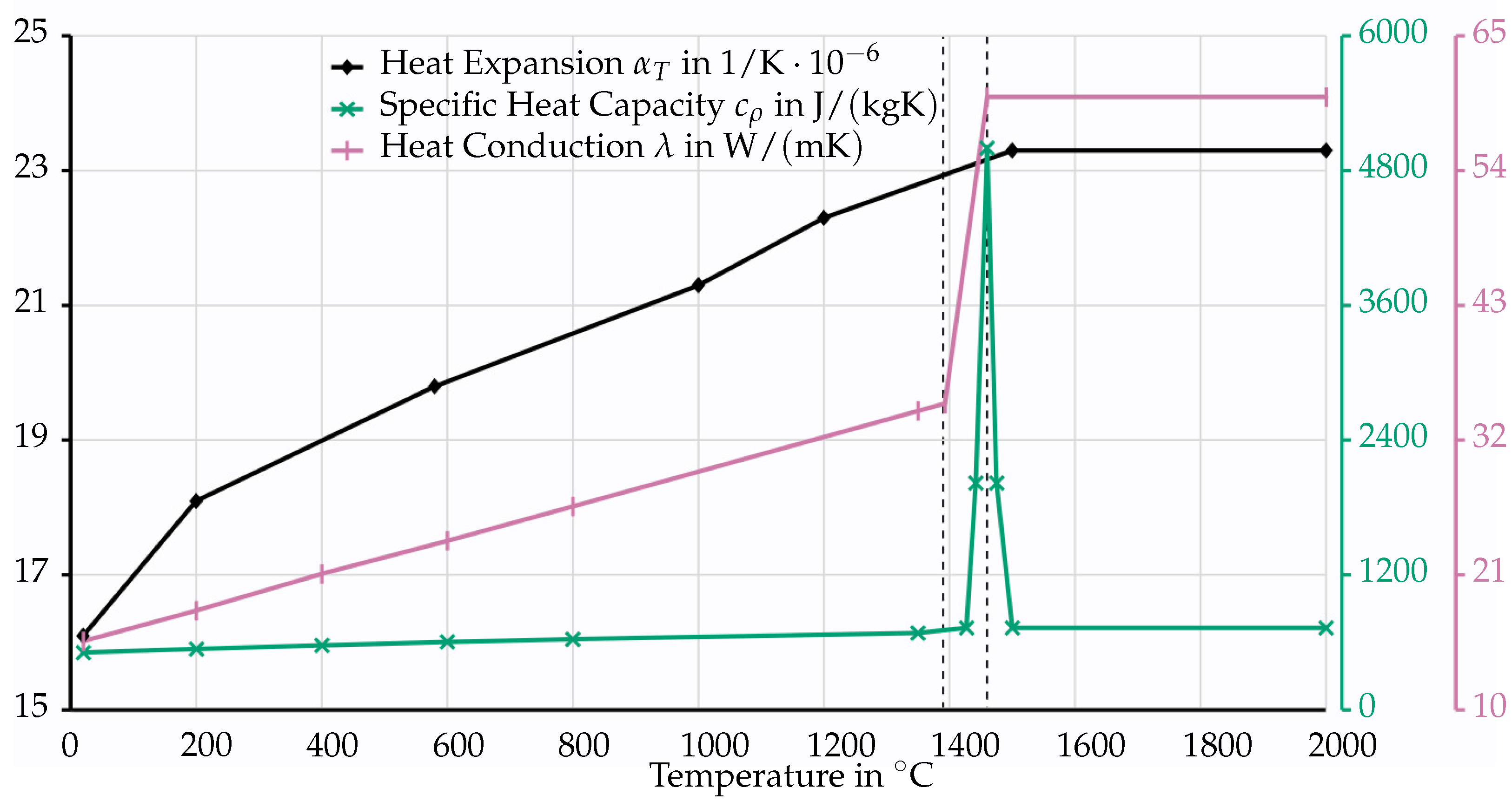
4.1. Material Modeling for Thermal Problem
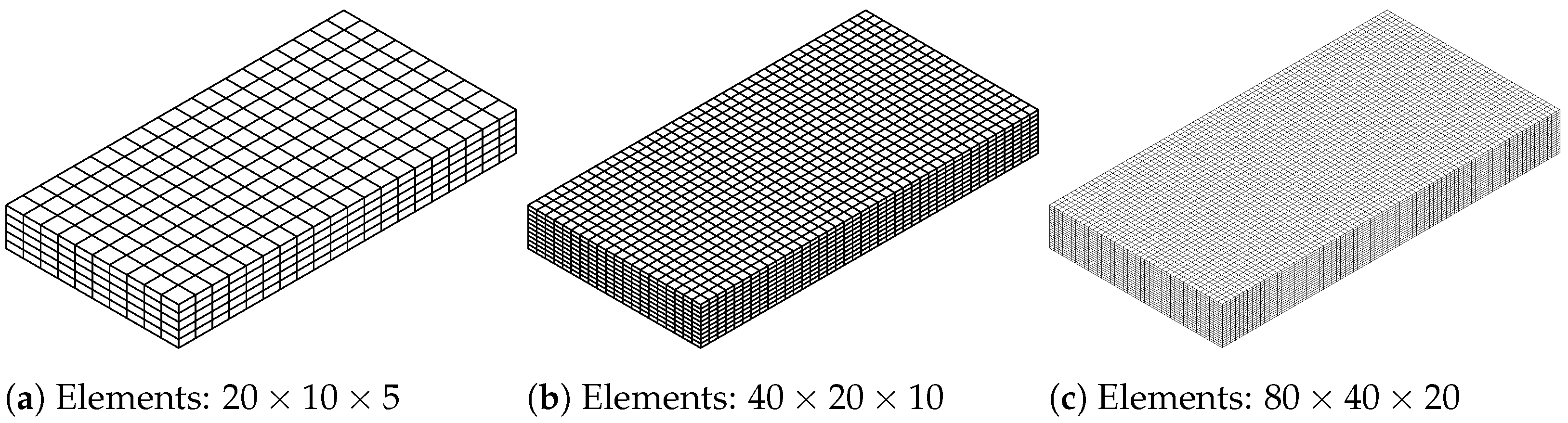
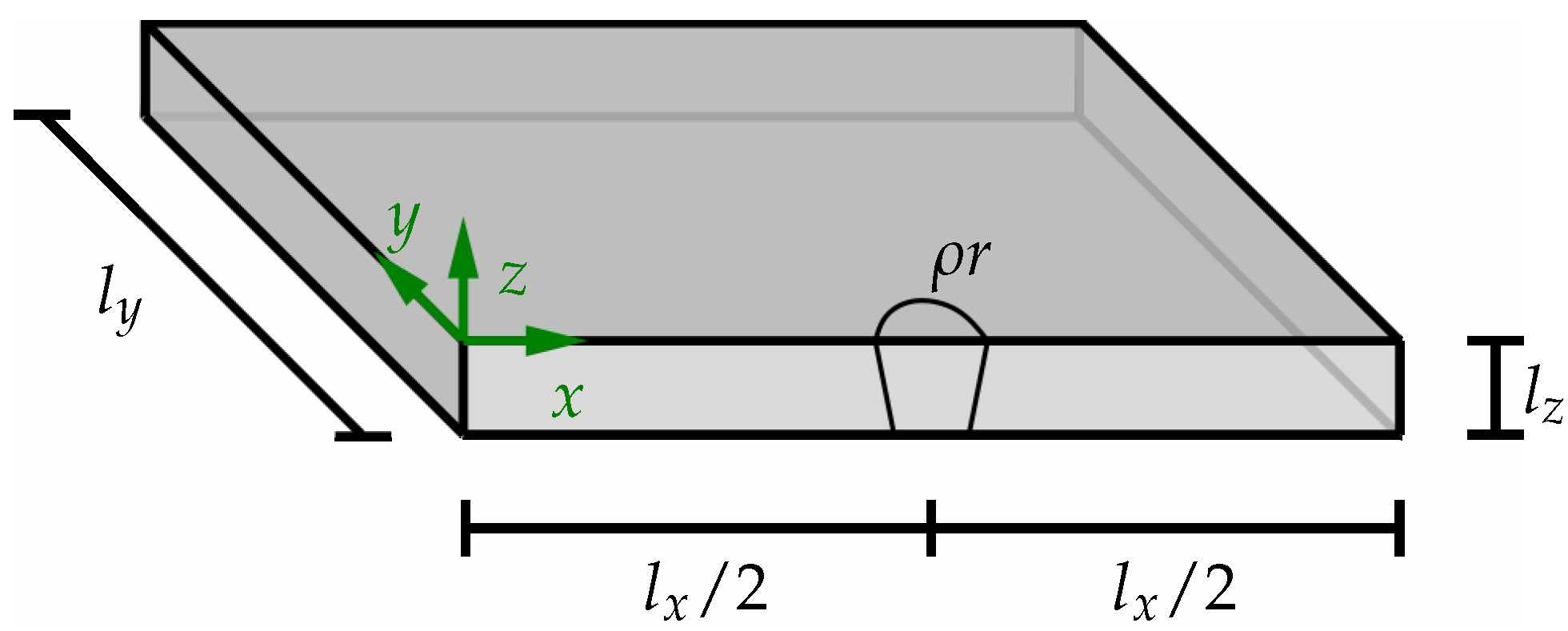
4.2. Finite-Element Discretization
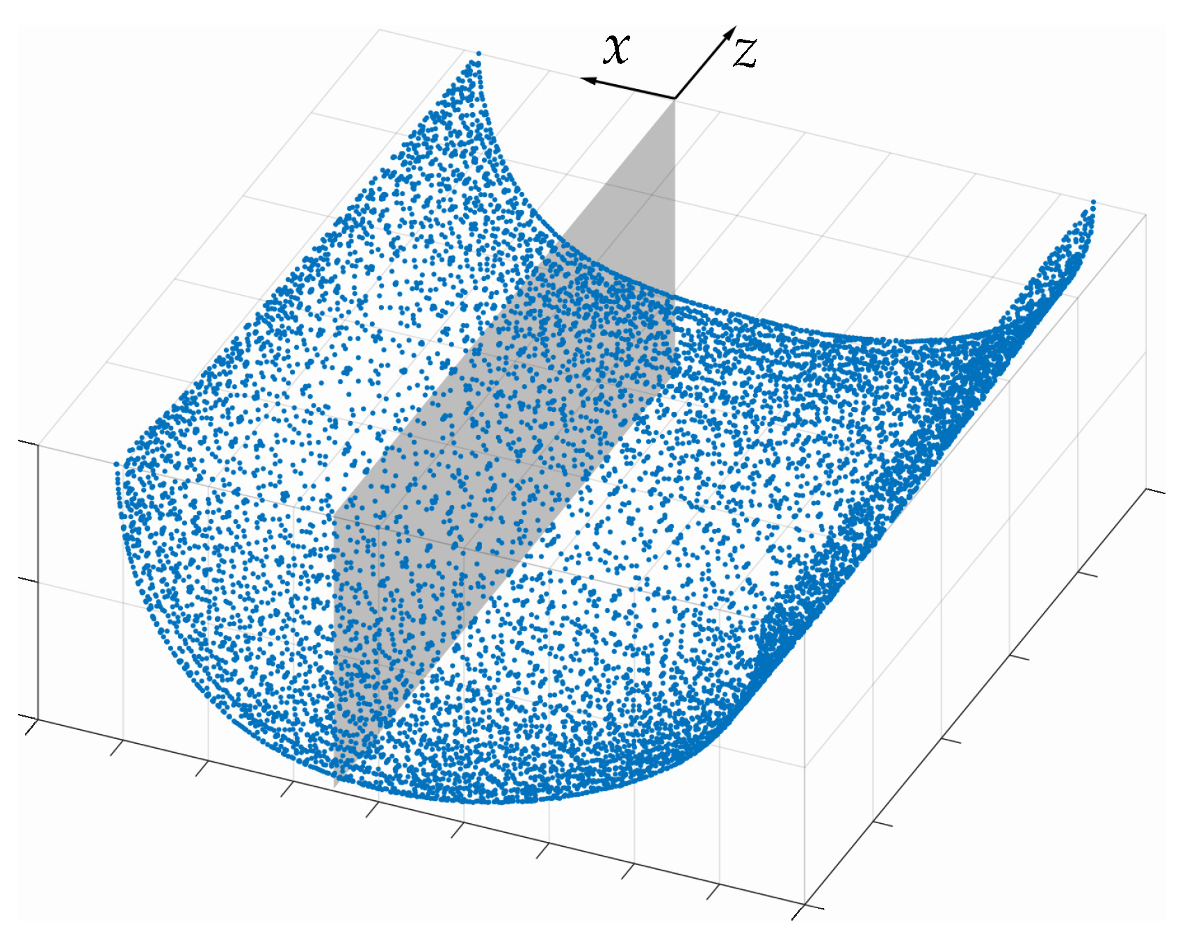
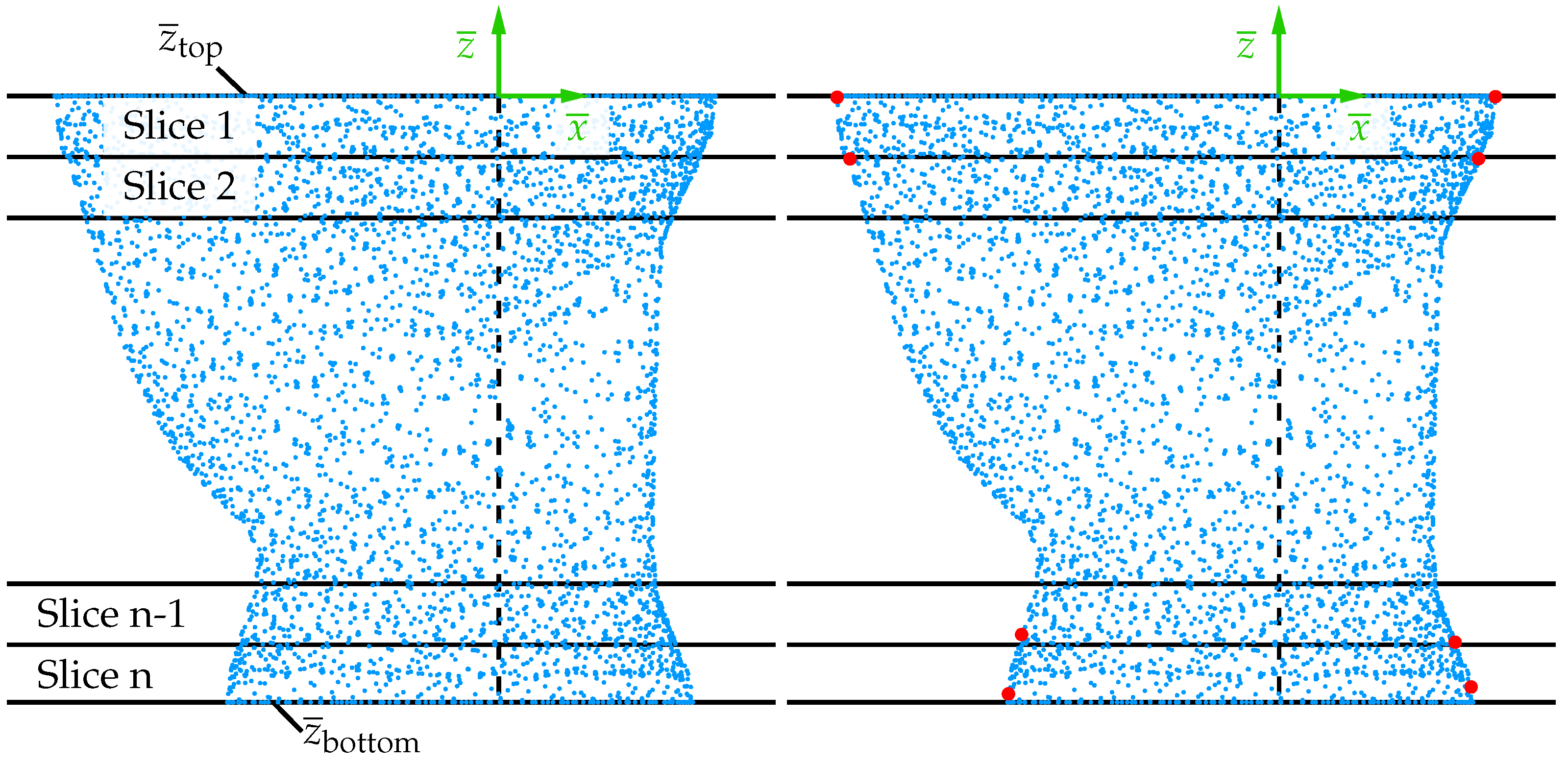
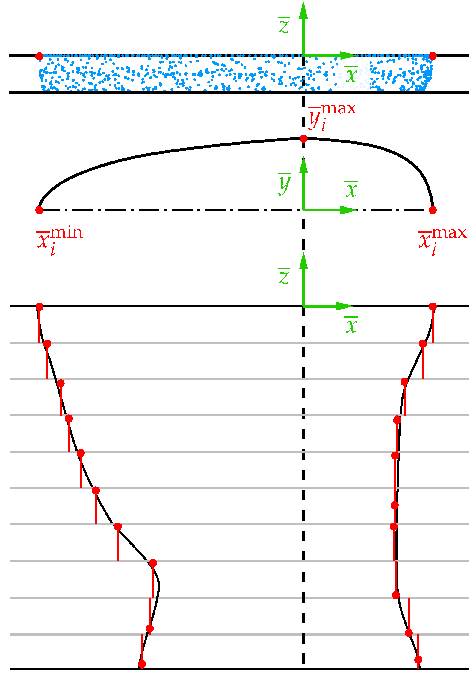
4.3. A Physically Motivated Heat Source Model Based on CFD Simulation
5. Numerical Examples
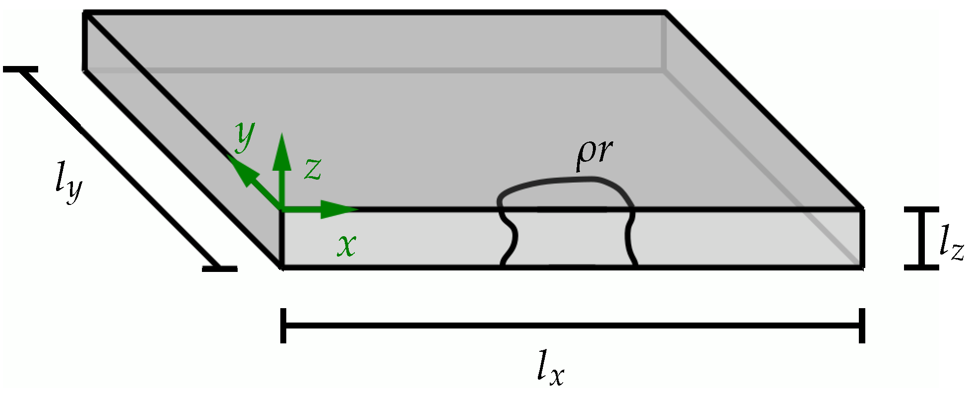
5.1. Material and Process Parameters
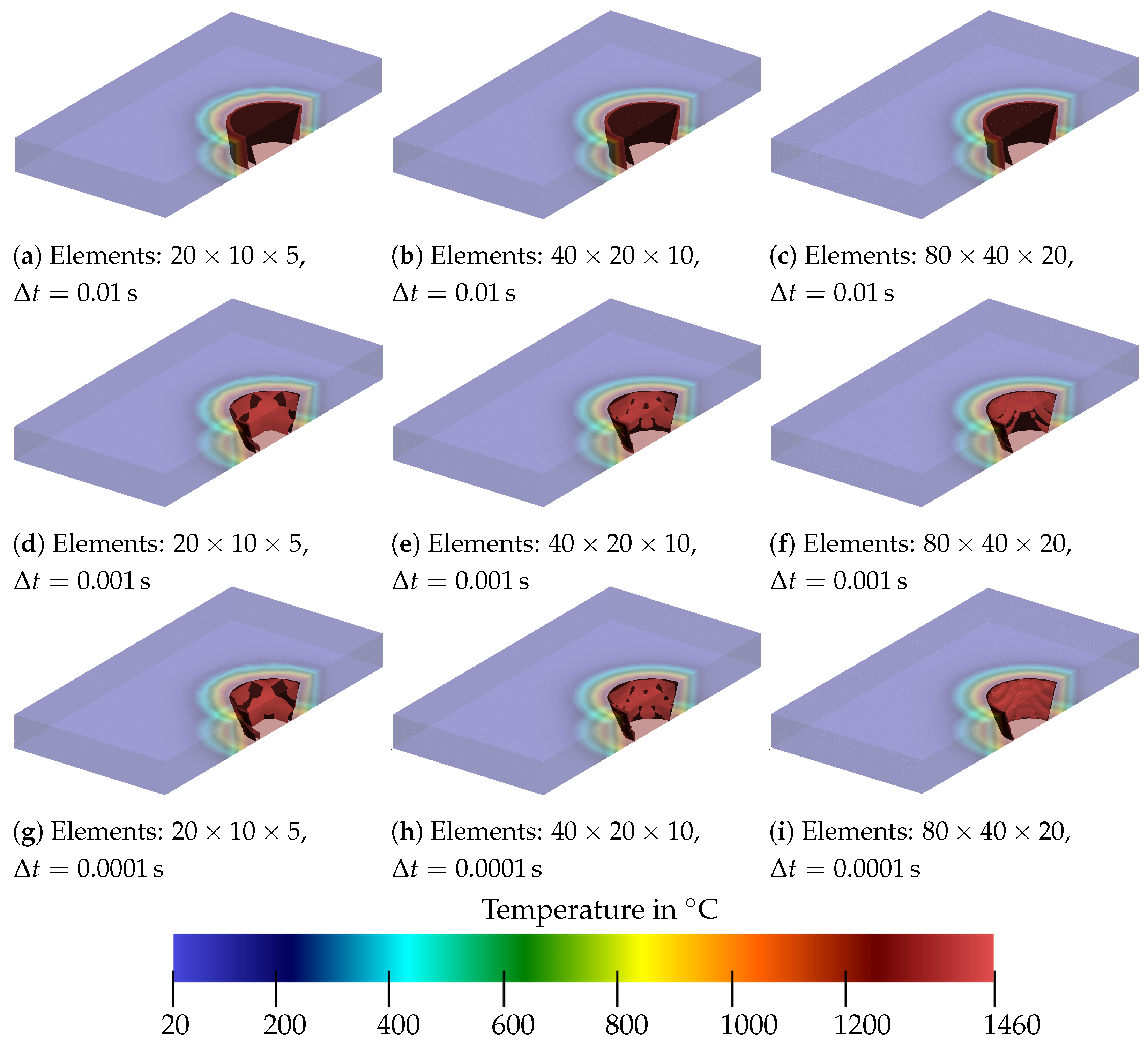
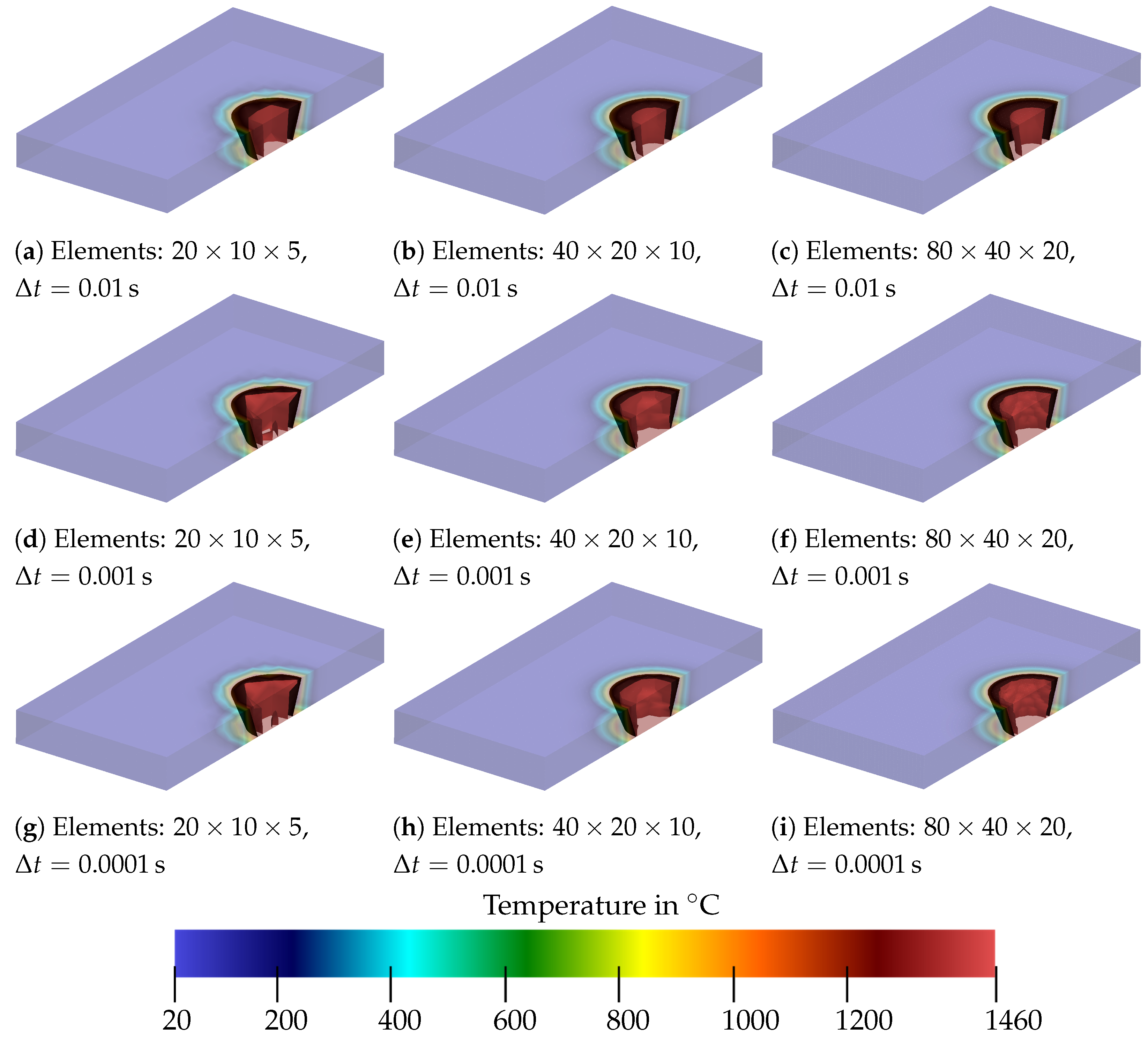
5.2. Analysis of Steady Conical Heat Source
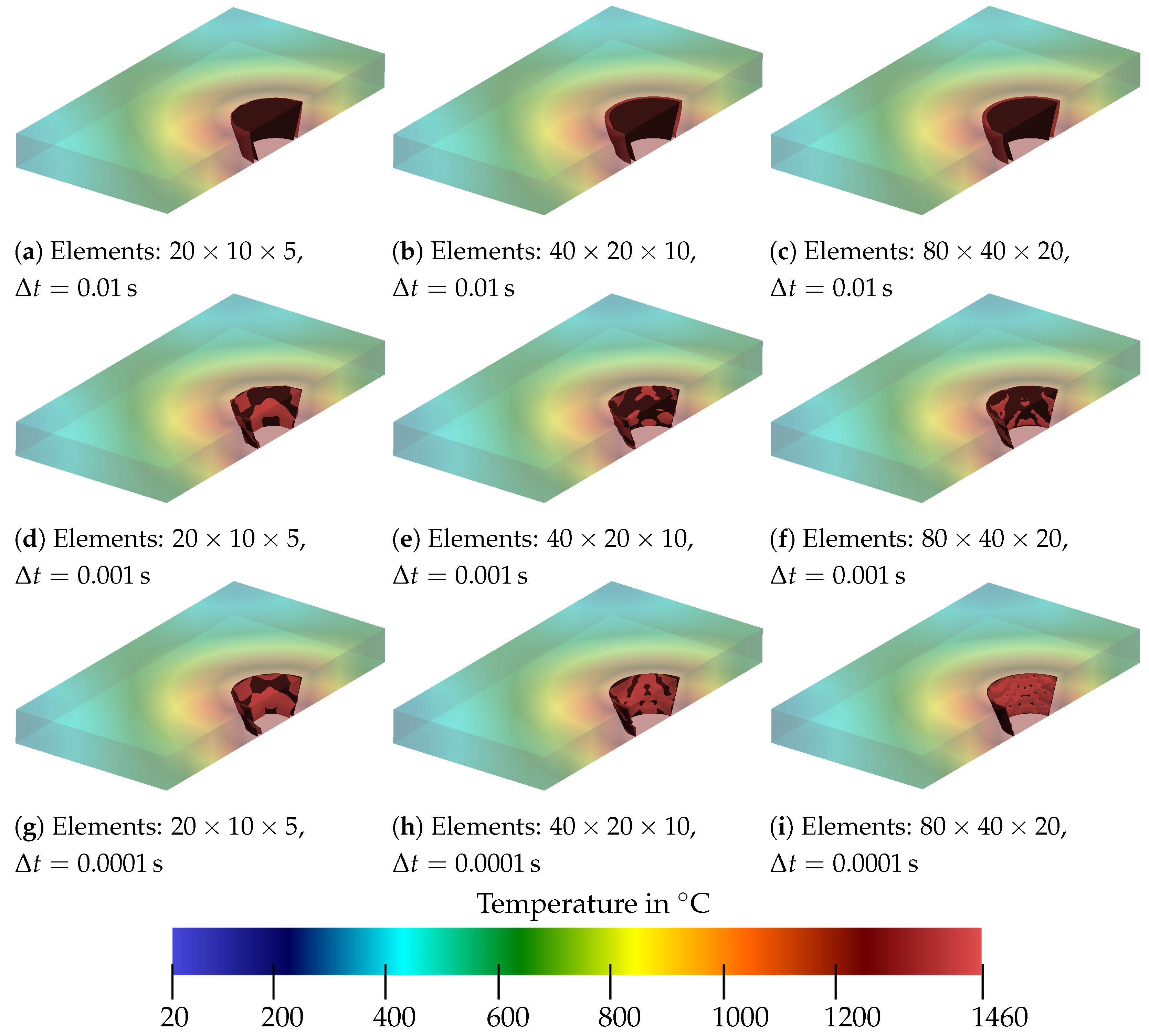
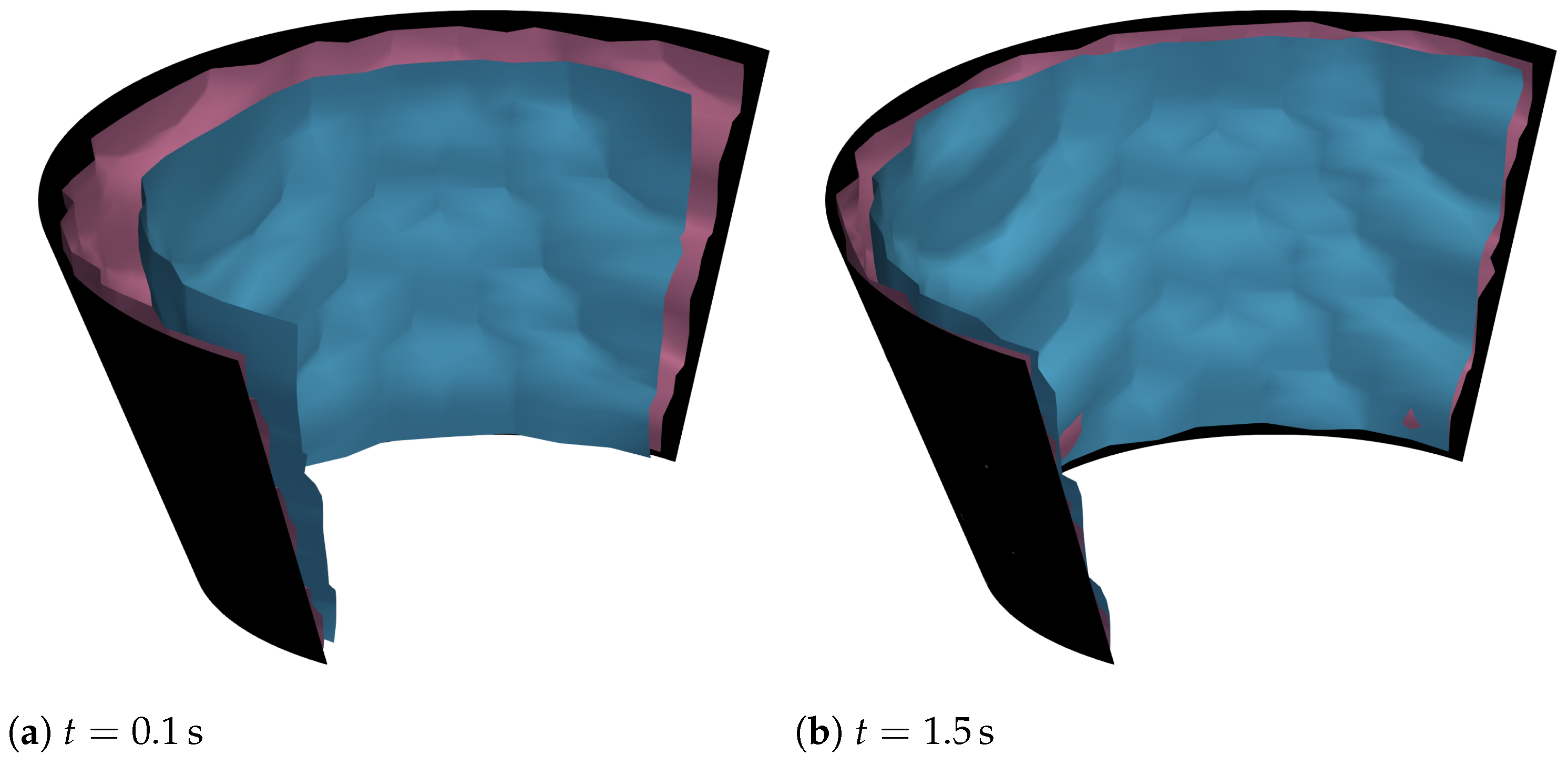
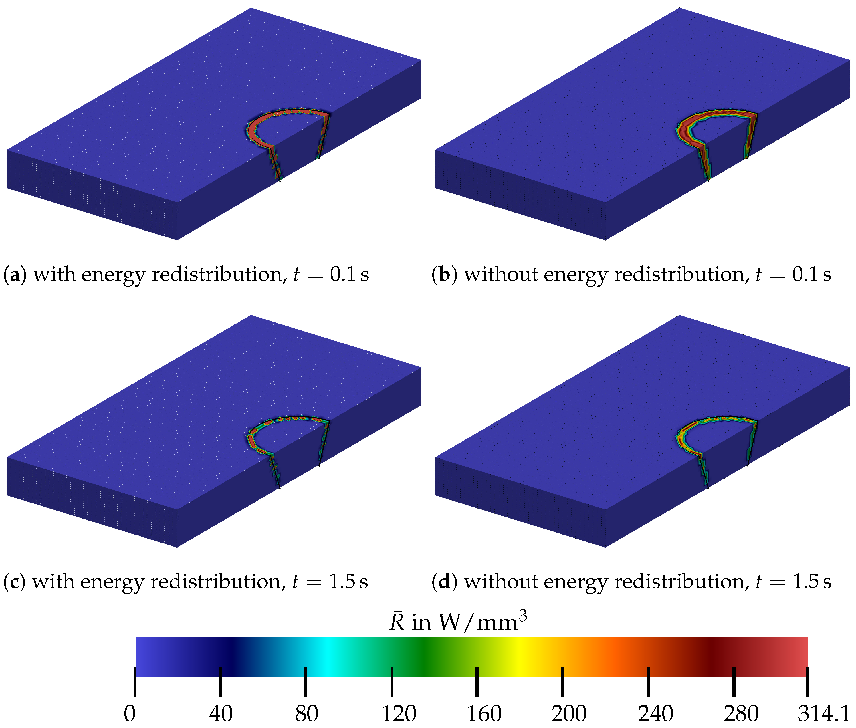
5.3. Moving Heat Source
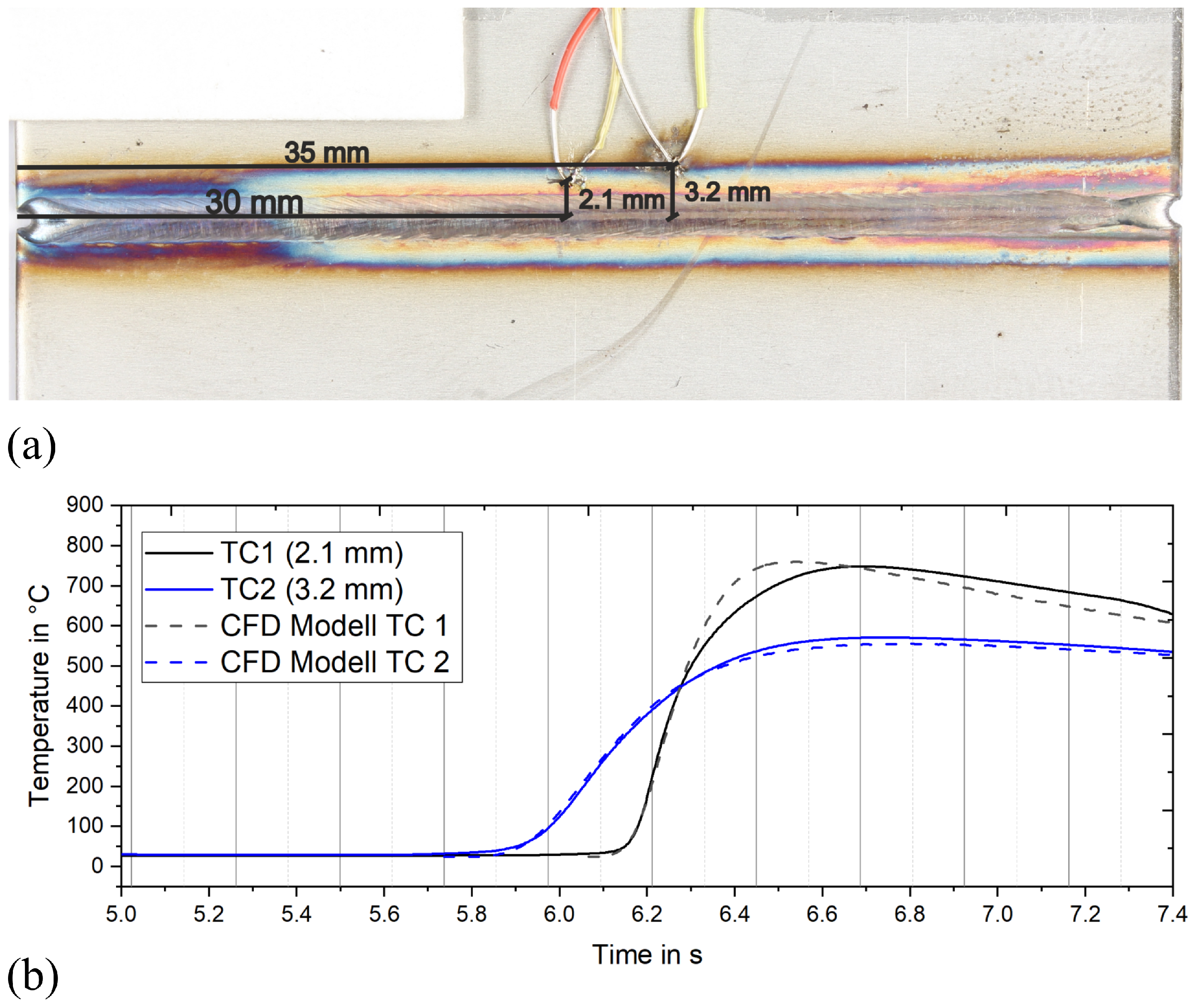
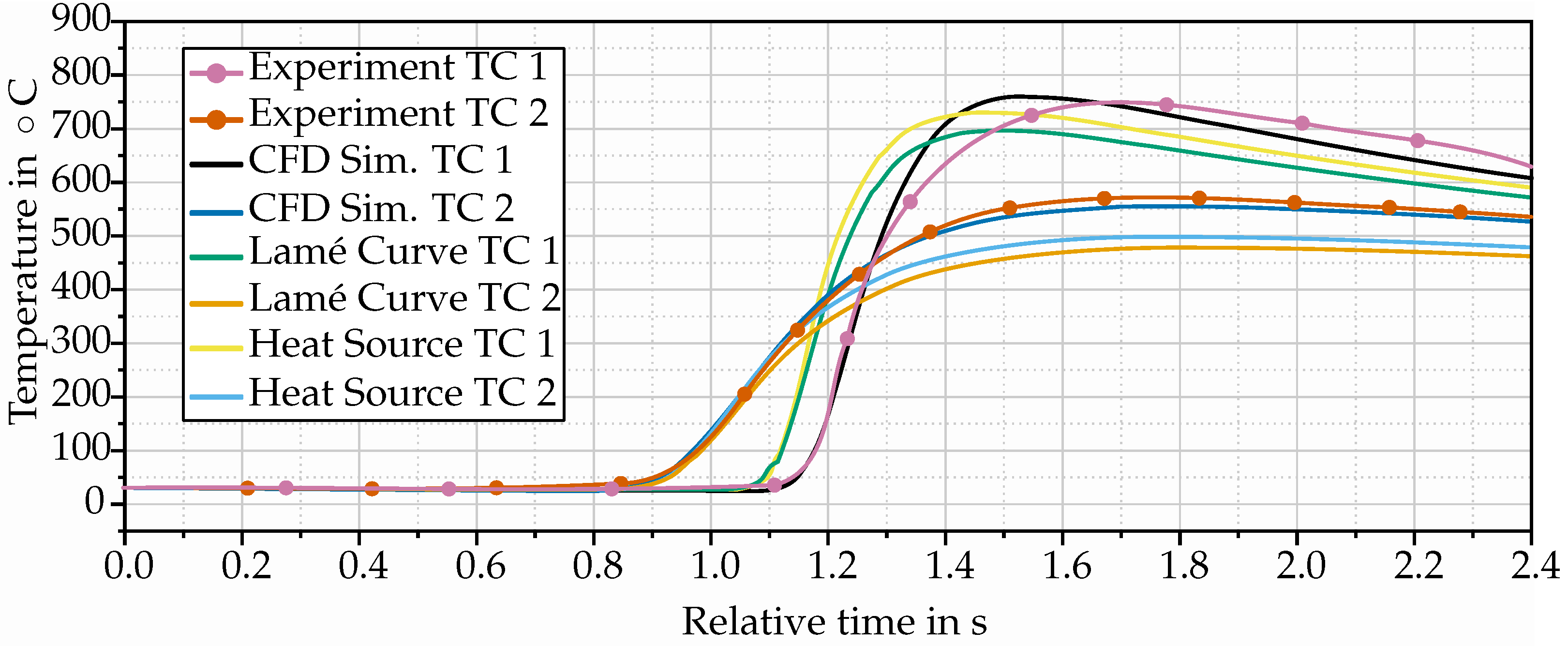
Comparison of Finite-Element Results to Experimental Data and CFD Simulations
6. Summary and Discussion
Author Contributions
Funding
Data Availability Statement
Conflicts of Interest
Abbreviations
| BAM | Bundesanstalt für Materialforschung und -prüfung |
| BVP | boundary-value problem |
| CFD | Computational Fluid Dynamics |
| FE | finite element |
| FEM | Finite-Element Method |
| RANS | Reynolds-averaged Navier–Stokes |
| TC | Thermocouple |
References
- Dilthey, U. Schweißtechnische Fertigungsverfahren 1: Schweiß- und Schneidtechnologien, 3rd ed.; VDI-Buch; Springer: Berlin/Heidelberg, Germany, 2006. [Google Scholar]
- Hills, R.N.; Loper, D.E.; Roberts, P.H. A thermodynamically consistent model of a mushy zone. Q. J. Mech. Appl. Math. 1983, 36, 505–540. [Google Scholar] [CrossRef]
- Yoshioka, H.; Tada, Y.; Hayashi, Y. Crystal growth and its morphology in the mushy zone. Acta Mater. 2004, 52, 1515–1523. [Google Scholar] [CrossRef]
- Rosenthal, D. The theory of moving sources of heat and its application to metal treatments. Trans. Am. Soc. Mech. Eng. 1946, 68, 849–865. [Google Scholar] [CrossRef]
- Boulton, N.; Martin, H.L. Residual stresses in arc-welded plates. Proc. Inst. Mech. Eng. 1936, 133, 295–347. [Google Scholar] [CrossRef]
- Bruce, W. The thermal distribution and temperature gradient in the arc welding of oil well casing. J. Appl. Phys. 1939, 10, 578–584. [Google Scholar] [CrossRef]
- Mahla, E.M. Heat Flow in Arc Welding. Ph.D. Thesis, Lehigh University, Bethlehem, PA, USA, 1941. [Google Scholar]
- Eagar, T.; Tsai, N. Temperature fields produced by traveling distributed heat sources. Weld. J. 1983, 62, 346–355. [Google Scholar]
- Pavelic, V.; Tanbakuchi, R.; Uyehara, O.; Myers, P. Experimental and computed temperature histories in gas tungsten arc welding of thin plates. Weld. J. Res. Suppl. 1969, 48, 296–305. [Google Scholar]
- Wu, C.; Wang, H.; Zhang, Y. A New Heat Source Model for Keyhole Plasma Arc Welding in FEM Analysis of the Temperature Profile. Weld. J. 2006, 85, 284. [Google Scholar]
- Goldak, J.; Chakravarti, A.; Bibby, M. A new finite element model for welding heat sources. Metall. Trans. B 1984, 15, 299–305. [Google Scholar] [CrossRef]
- Rahman Chukkan, J.; Vasudevan, M.; Muthukumaran, S.; Ravi Kumar, R.; Chandrasekhar, N. Simulation of laser butt welding of AISI 316L stainless steel sheet using various heat sources and experimental validation. J. Mater. Process. Technol. 2015, 219, 48–59. [Google Scholar] [CrossRef]
- Farias, R.; Teixeira, P.; Vilarinho, L. Variable profile heat source models for numerical simulations of arc welding processes. Int. J. Therm. Sci. 2022, 179, 107593. [Google Scholar] [CrossRef]
- Winczek, J. The influence of the heat source model selection on mapping of heat affected zones during surfacing by welding. J. Appl. Math. Comput. Mech. 2016, 15, 167–178. [Google Scholar] [CrossRef]
- Heinze, C.; Schwenk, C.; Rethmeier, M. Effect of heat source configuration on the result quality of numerical calculation of welding-induced distortion. Simul. Model. Pract. Theory 2012, 20, 112–123. [Google Scholar] [CrossRef]
- Beygi, R.; Marques, E.; da Silva, L.F. Computational Concepts in Simulation of Welding Processes; Springer: Cham, Switzerland, 2022. [Google Scholar]
- Lazov, L.; Teirumnieks, E.; Draganov, I.; Angelov, N. Numerical modeling and simulation for laser beam welding of ultrafine-grained aluminium. Laser Phys. 2021, 31, 066001. [Google Scholar] [CrossRef]
- Fan, X.; Qin, G.; Jiang, Z.; Wang, H. Comparative analysis between the laser beam welding and low current pulsed GMA assisted high-power laser welding by numerical simulation. J. Mater. Res. Technol. 2023, 22, 2549–2565. [Google Scholar] [CrossRef]
- Duggirala, A.; Kalvettukaran, P.; Acherjee, B.; Mitra, S. Numerical simulation of the temperature field, weld profile, and weld pool dynamics in laser welding of aluminium alloy. Optik 2021, 247, 167990. [Google Scholar] [CrossRef]
- Yan, S.; Meng, Z.; Chen, B.; Tan, C.; Song, X.; Wang, G. Prediction of temperature field and residual stress of oscillation laser welding of 316LN stainless steel. Opt. Laser Technol. 2022, 145, 107493. [Google Scholar] [CrossRef]
- de Oliveira, A.F.M.; Magalhães, E.d.S.; Paes, L.E.d.S.; Pereira, M.; da Silva, L.R. A Thermal Analysis of LASER Beam Welding Using Statistical Approaches. Processes 2023, 11, 2023. [Google Scholar] [CrossRef]
- Artinov, A.; Karkhin, V.; Bakir, N.; Meng, X.; Bachmann, M.; Gumenyuk, A.; Rethmeier, M. Lamé curve approximation for the assessment of the 3D temperature distribution in keyhole mode welding processes. J. Laser Appl. 2020, 32, 022042. [Google Scholar] [CrossRef]
- Artinov, A.; Bachmann, M.; Rethmeier, M. Equivalent heat source approach in a 3D transient heat transfer simulation of full-penetration high power laser beam welding of thick metal plates. Int. J. Heat Mass Transf. 2018, 122, 1003–1013. [Google Scholar] [CrossRef]
- Hildebrand, J. Numerische Schweißsimulation-Bestimmung von Temperatur, Gefüge und Eigenspannung an Schweißverbindungen aus Stahl-und Glaswerkstoffen. Ph.D. Thesis, Bauhaus-Universität Weimar, Weimar, Germany, 2008. [Google Scholar]
- Sahoo, P.; Debroy, T.; McNallan, M. Surface tension of binary metal—Surface active solute systems under conditions relevant to welding metallurgy. Metall. Trans. B 1988, 19, 483–491. [Google Scholar] [CrossRef]
- Simo, J.; Miehe, C. Associative coupled thermoplasticity at finite strains: Formulation, numerical analysis and implementation. Comput. Methods Appl. Mech. Eng. 1992, 98, 41–104. [Google Scholar] [CrossRef]
- Wriggers, P. Nonlinear Finite Element Methods; Springer Nature: Berlin/Heidelberg, Germany, 2008. [Google Scholar]
- Knothe, K.; Wessels, H. Finite Elemente: Eine Einführung für Ingenieure, 5th ed.; Springer: Berlin/Heidelberg, Germany, 2017. [Google Scholar]
- Zain-Ul-Abdein, M.; Nélias, D.; Jullien, J.; Deloison, D. Thermo-mechanical Analysis of Laser Beam Welding of Thin Plate with Complex Boundary Conditions. Int. J. Mater. Form. 2008, 1, 1063–1066. [Google Scholar] [CrossRef]
- Agarwal, G.; Gao, H.; Amirthalingam, M.; Hermans, M. Study of Solidification Cracking Susceptibility during Laser Welding in an Advanced High Strength Automotive Steel. Metals 2018, 8, 673. [Google Scholar] [CrossRef]
- Kik, T. Computational Techniques in Numerical Simulations of Arc and Laser Welding Processes. Materials 2020, 13, 608. [Google Scholar] [CrossRef] [PubMed]
- Kik, T. Heat Source Models in Numerical Simulations of Laser Welding. Materials 2020, 13, 2653. [Google Scholar] [CrossRef] [PubMed]
- Taylor, R. FEAP—A Finite Element Analysis Program, Version 8.2. Department of Civil and Environmental Engineering, University of California at Berkley, Berkley, California 94720-1710, March 2008. Available online: http://projects.ce.berkeley.edu/feap/ (accessed on 18 March 2024).
- Sente Software Ltd. JMatPro; Sente Software Ltd.: Guildford, UK, 2022. [Google Scholar]
- Richter, F. Die physikalischen Eigenschaften der Stähle—Das 100 Stähle-Programm; Technical Report; TU Graz: Styria, Austria, 2011. [Google Scholar]
- Geuzaine, C.; Remacle, J.-F. Gmsh: A 3-D finite element mesh generator with built-in pre- and post-processing facilities. Int. J. Numer. Methods Eng. 2009, 79, 1309–1331. [Google Scholar] [CrossRef]
- Bakir, N.; Artinov, A.; Gumenyuk, A.; Bachmann, M.; Rethmeier, M. Numerical simulation on the origin of solidification cracking in laser welded thick-walled structures. Metals 2018, 8, 406. [Google Scholar] [CrossRef]


| Element | C | Si | Mn | P | S | Cr | N | Ni | Fe |
|---|---|---|---|---|---|---|---|---|---|
| wt% | 0.02 | 0.41 | 1.6 | 0.028 | <0.002 | 19.09 | 0.095 | 8.06 | bal. |
| Material Property | Symbol | Value | Unit |
|---|---|---|---|
| Mass density | 8030 | kg m−3 | |
| Melting temperature | 1733 | K | |
| Evaporation temperature | 3000 | K | |
| Latent heat of fusion | J kg−1 | ||
| Marangoni coefficient | N m−1 K−1 | ||
| Heat transfer coefficient (air) | h | 15 | W m−2 K−1 |
| Material properties at | |||
| Mass density | 6900 | kg m−3 | |
| Dynamic viscosity | Pa s | ||
| Thermal conductivity | 150 | W m−1 K−1 | |
| Specific heat capacity | 800 | J kg−1 K−1 | |
Disclaimer/Publisher’s Note: The statements, opinions and data contained in all publications are solely those of the individual author(s) and contributor(s) and not of MDPI and/or the editor(s). MDPI and/or the editor(s) disclaim responsibility for any injury to people or property resulting from any ideas, methods, instructions or products referred to in the content. |
© 2024 by the authors. Licensee MDPI, Basel, Switzerland. This article is an open access article distributed under the terms and conditions of the Creative Commons Attribution (CC BY) license (https://creativecommons.org/licenses/by/4.0/).
Share and Cite
Hartwig, P.; Bakir, N.; Scheunemann, L.; Gumenyuk, A.; Schröder, J.; Rethmeier, M. A Physically Motivated Heat Source Model for Laser Beam Welding. Metals 2024, 14, 430. https://doi.org/10.3390/met14040430
Hartwig P, Bakir N, Scheunemann L, Gumenyuk A, Schröder J, Rethmeier M. A Physically Motivated Heat Source Model for Laser Beam Welding. Metals. 2024; 14(4):430. https://doi.org/10.3390/met14040430
Chicago/Turabian StyleHartwig, Philipp, Nasim Bakir, Lisa Scheunemann, Andrey Gumenyuk, Jörg Schröder, and Michael Rethmeier. 2024. "A Physically Motivated Heat Source Model for Laser Beam Welding" Metals 14, no. 4: 430. https://doi.org/10.3390/met14040430
APA StyleHartwig, P., Bakir, N., Scheunemann, L., Gumenyuk, A., Schröder, J., & Rethmeier, M. (2024). A Physically Motivated Heat Source Model for Laser Beam Welding. Metals, 14(4), 430. https://doi.org/10.3390/met14040430