
Sensitivity Analysis of the Square Cup Forming Process Using PAWN and Sobol Indices

 ,
,  ,
,  ,
,  and
and
Abstract
1. Introduction
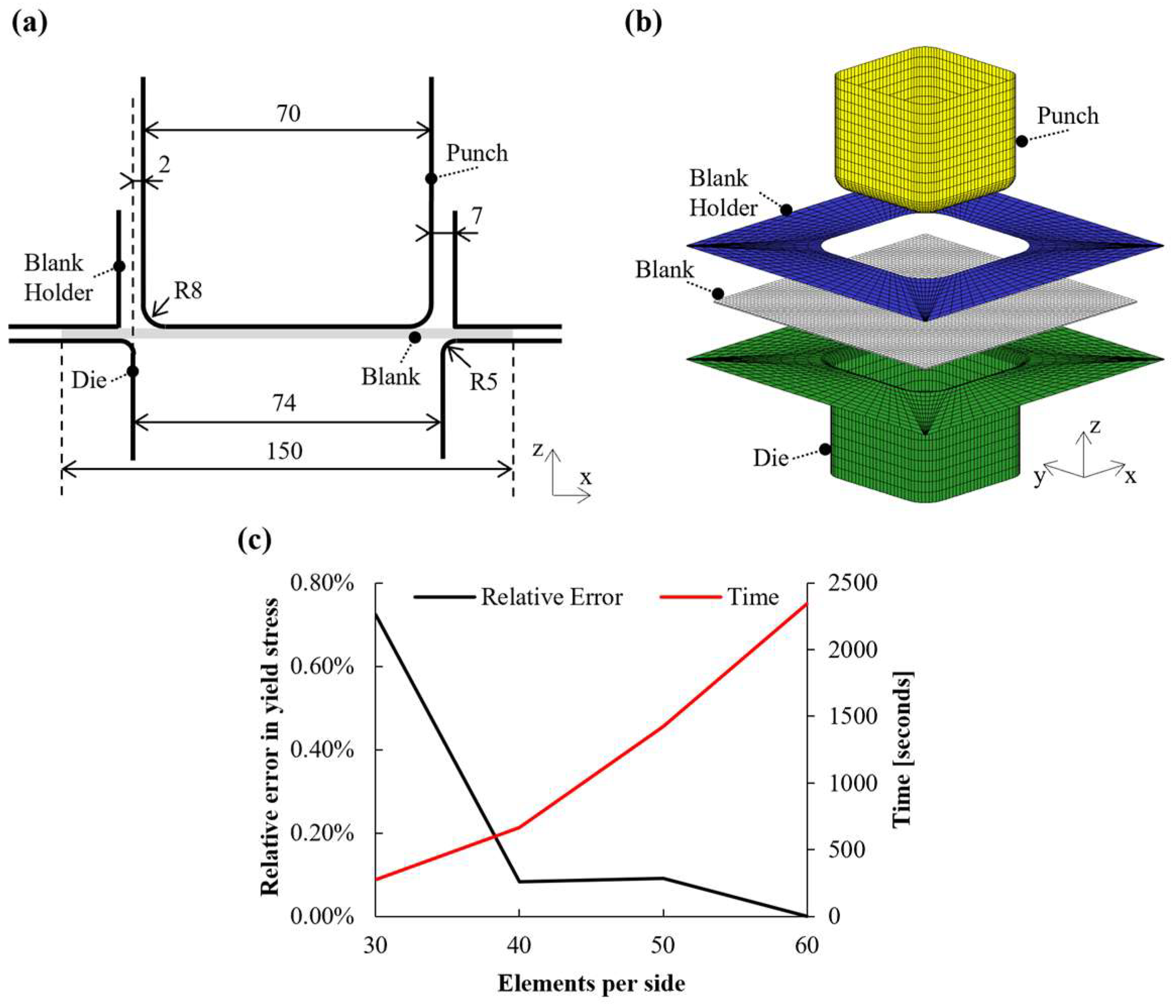
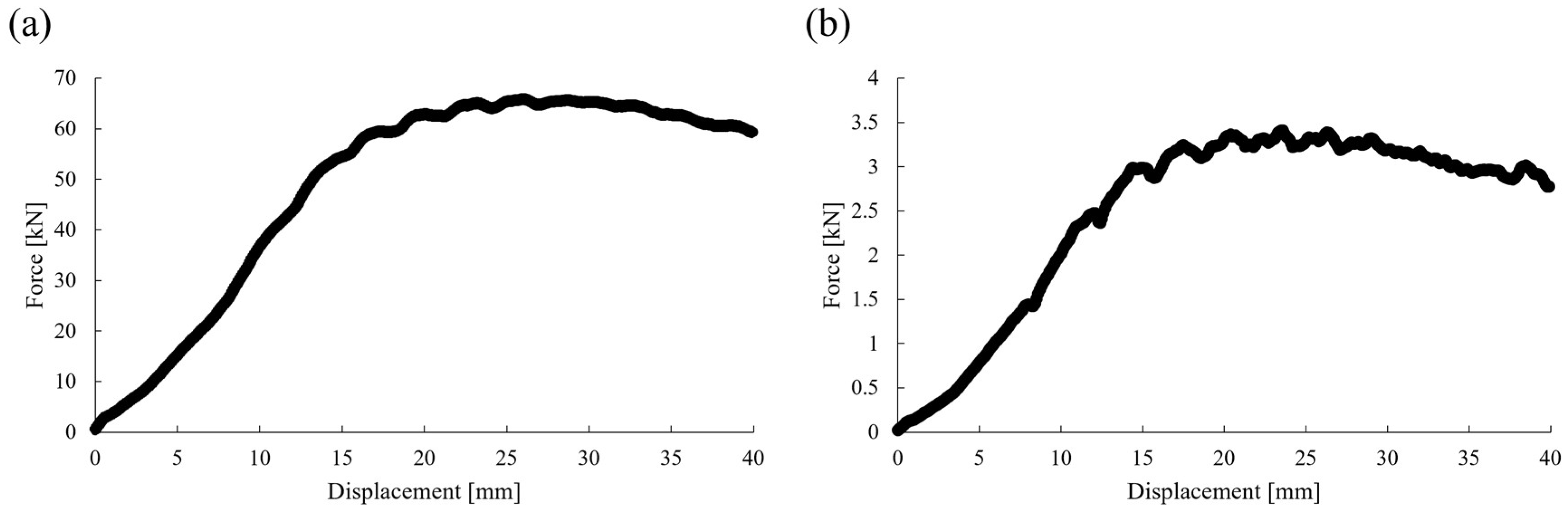
2. Numerical Model
3. Sensitivity Analysis
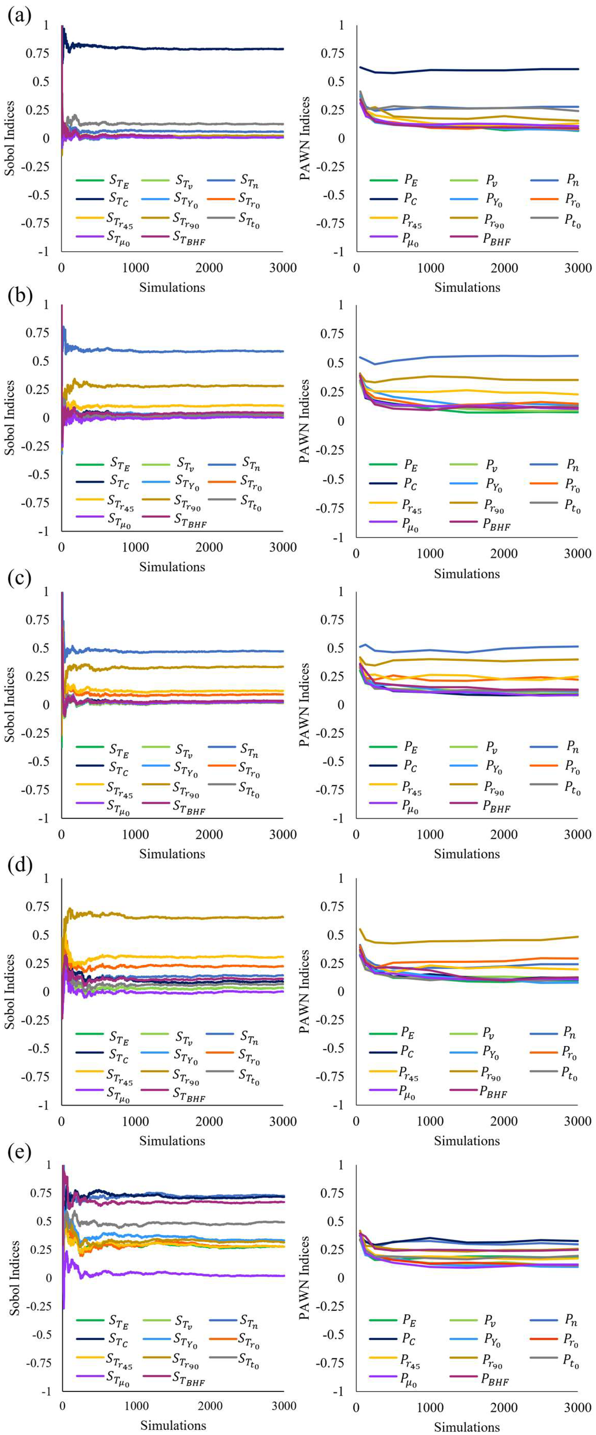
3.1. Stabilization Analysis
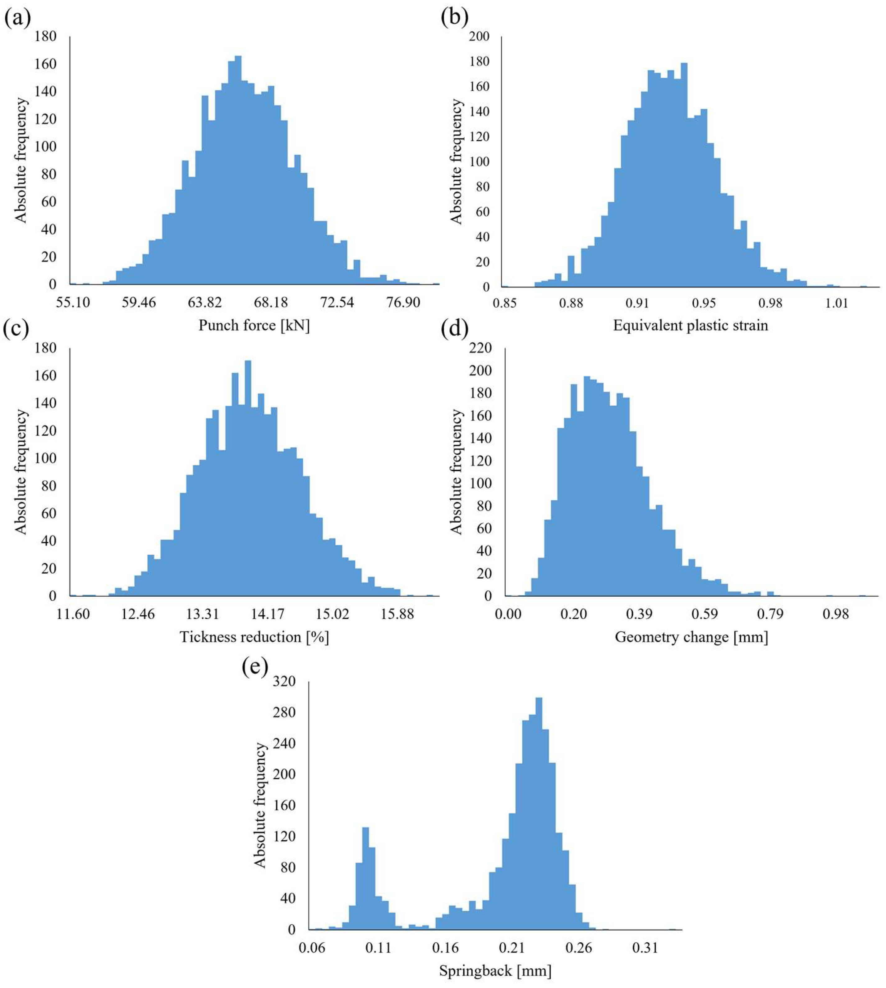
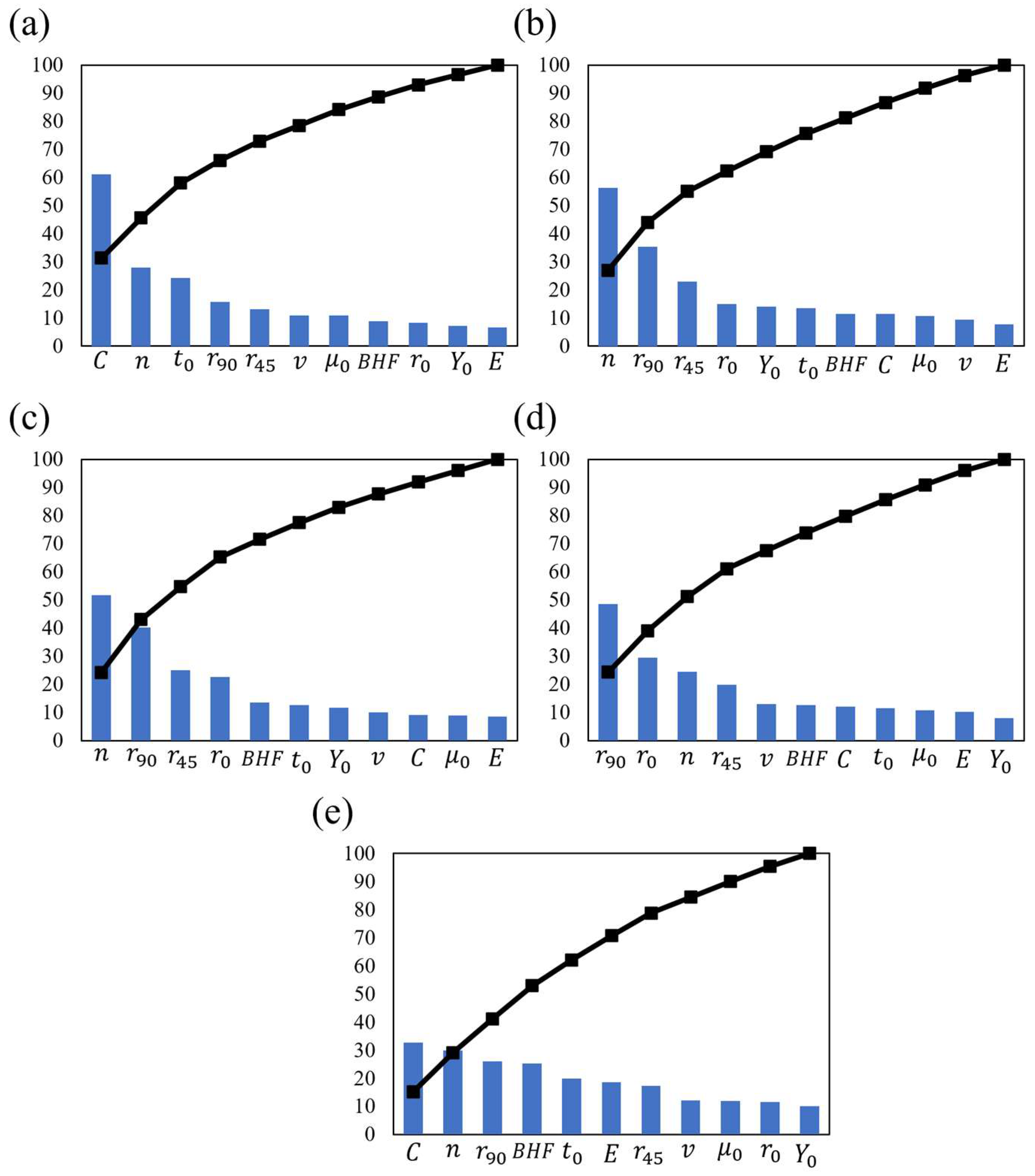
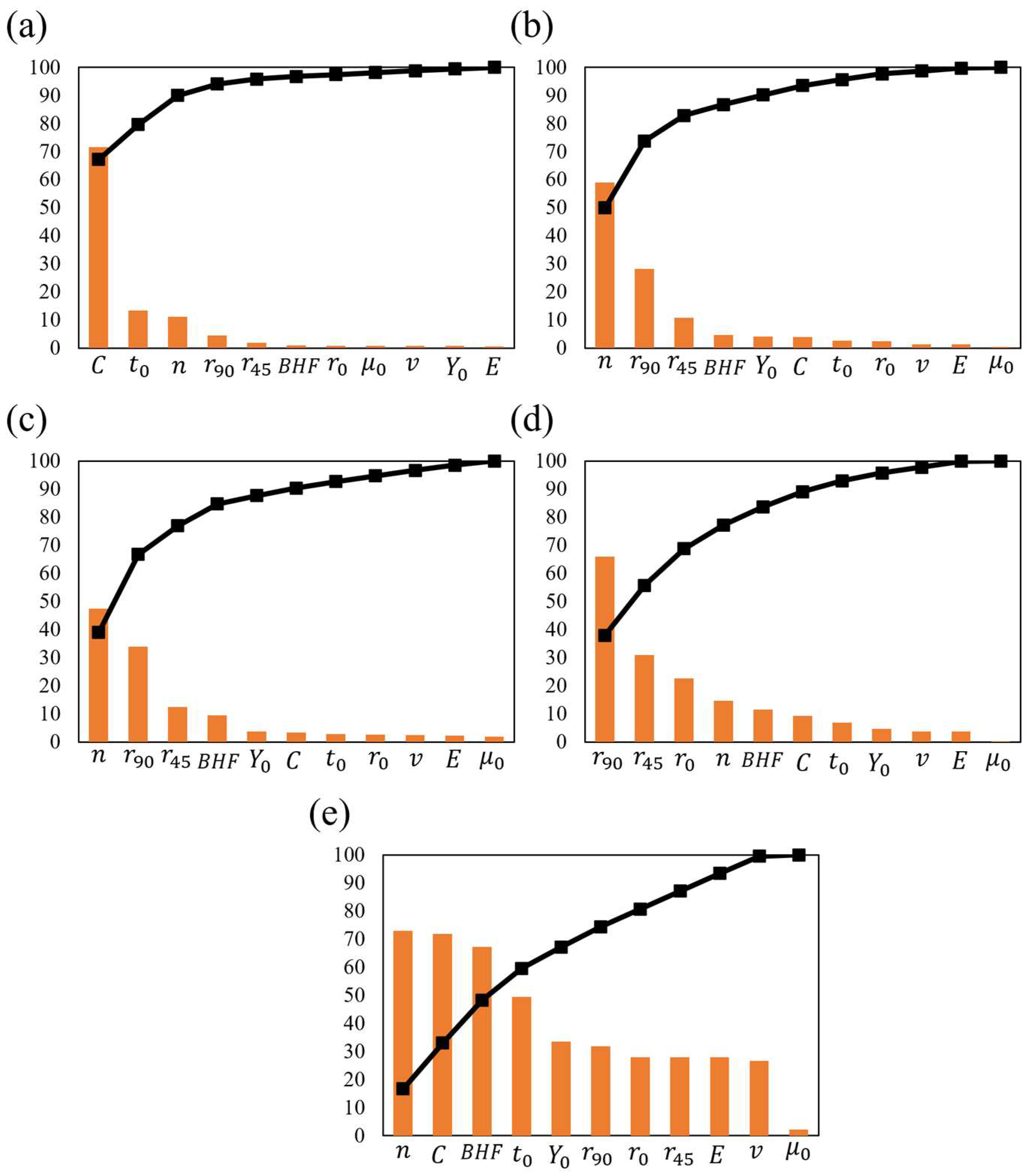
3.2. Pareto Analysis
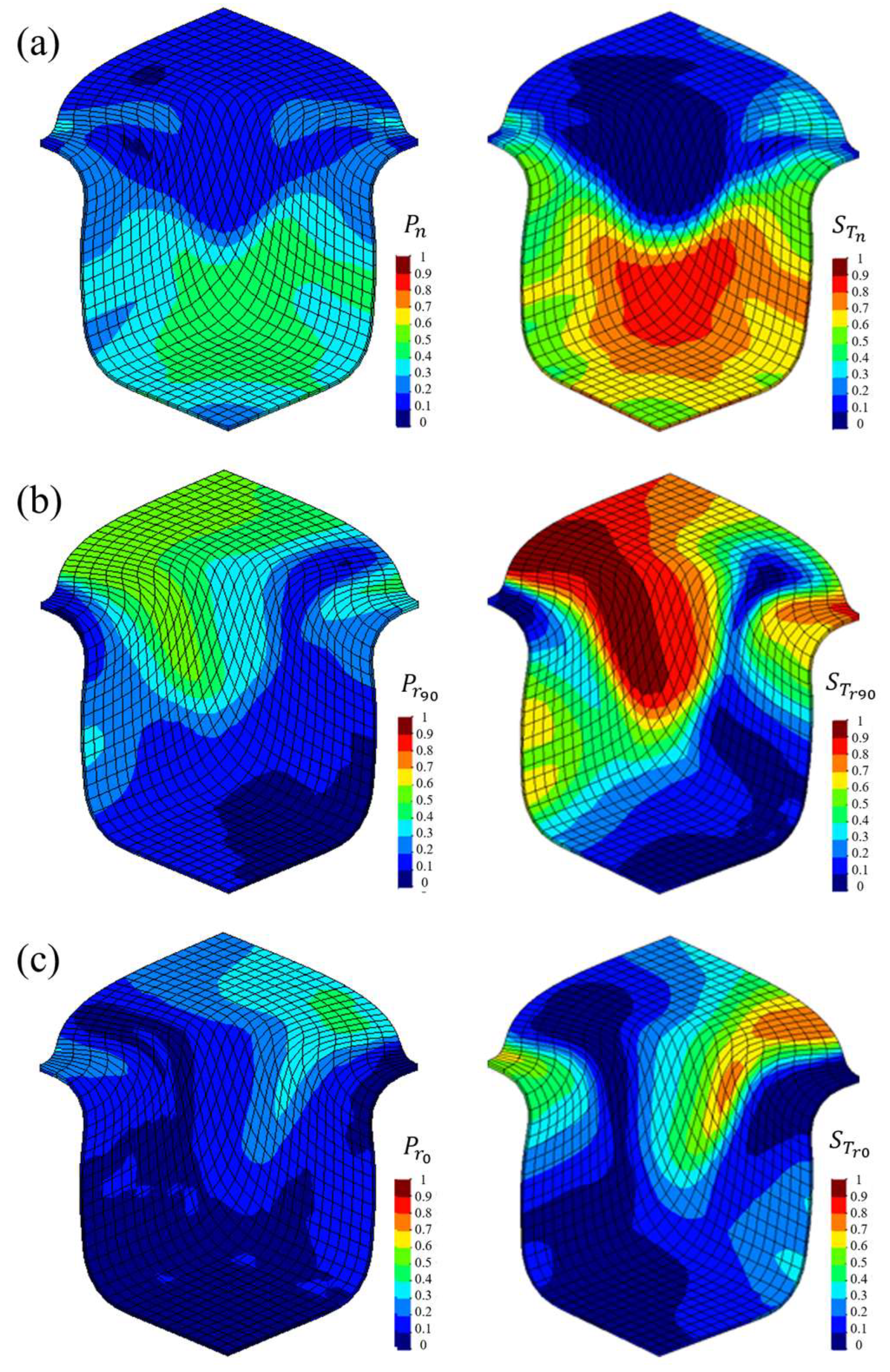
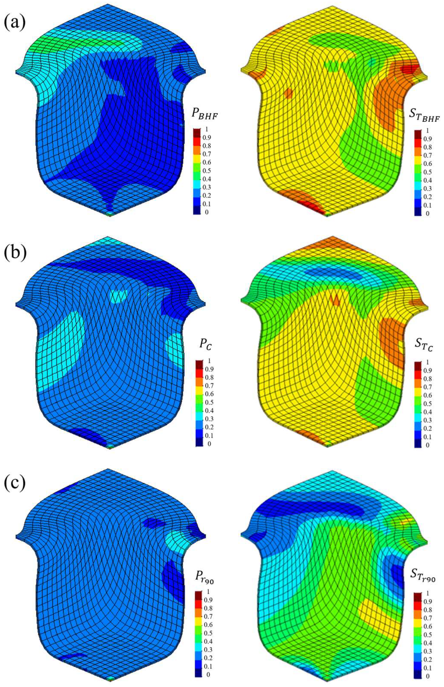
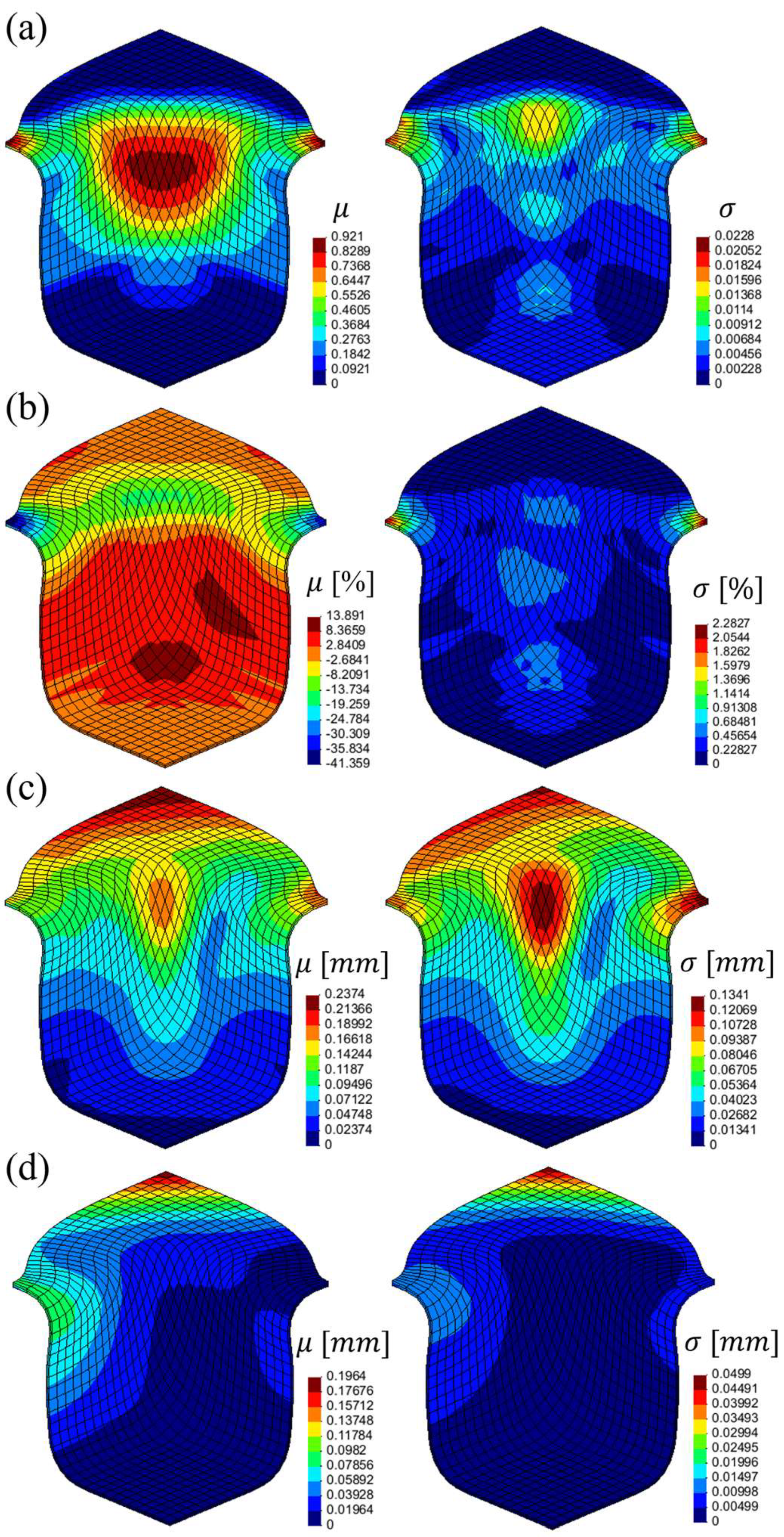
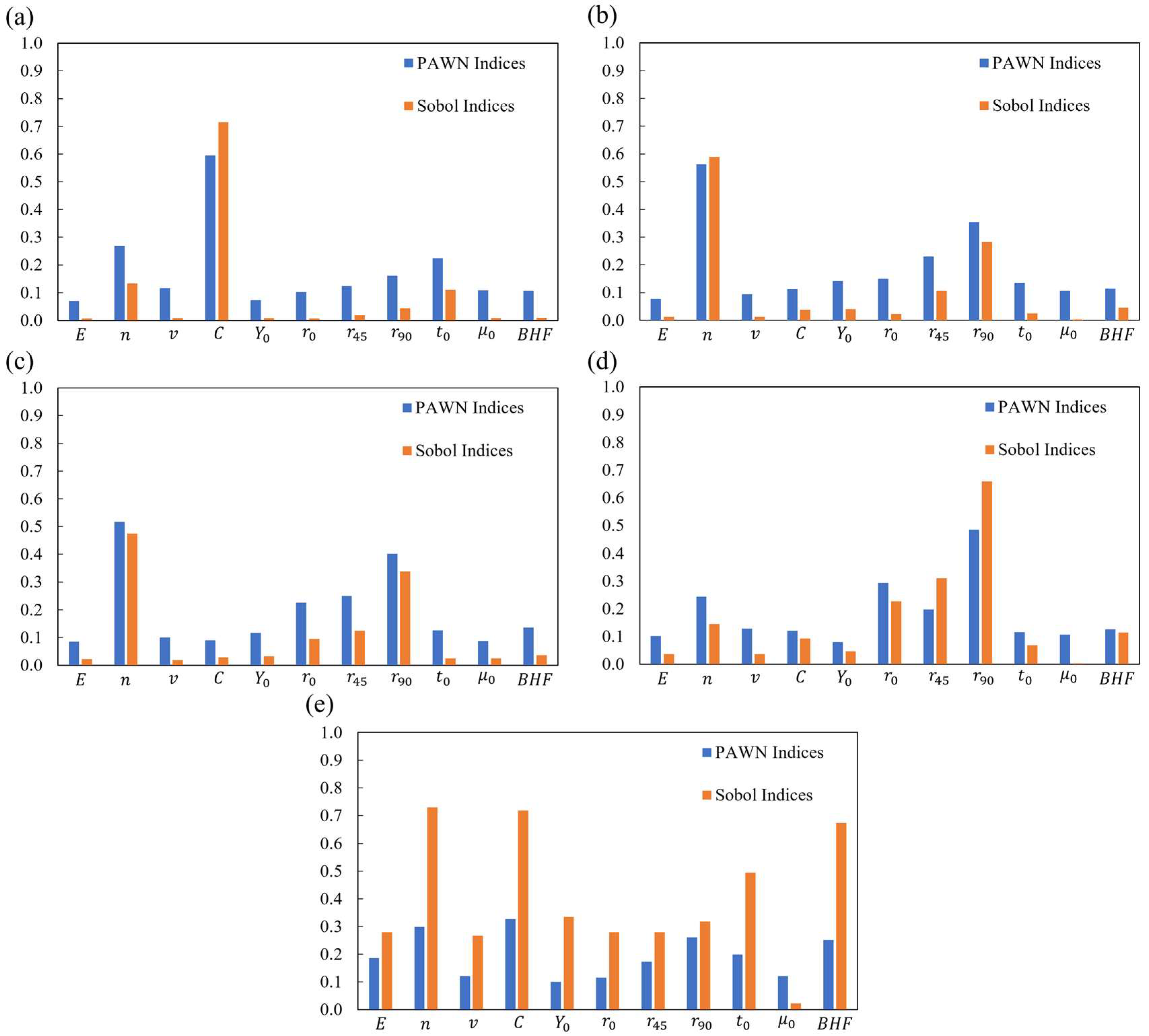
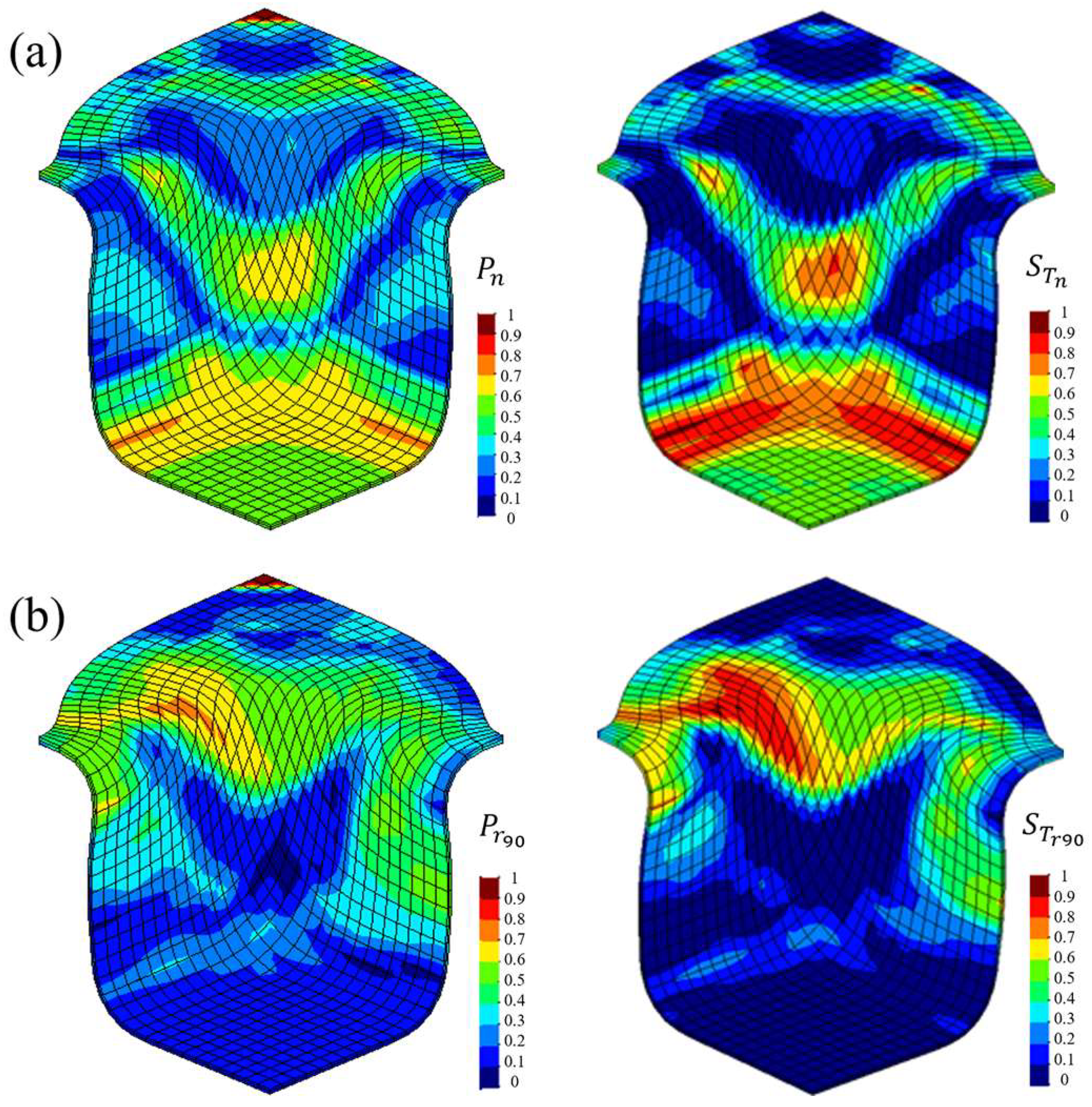
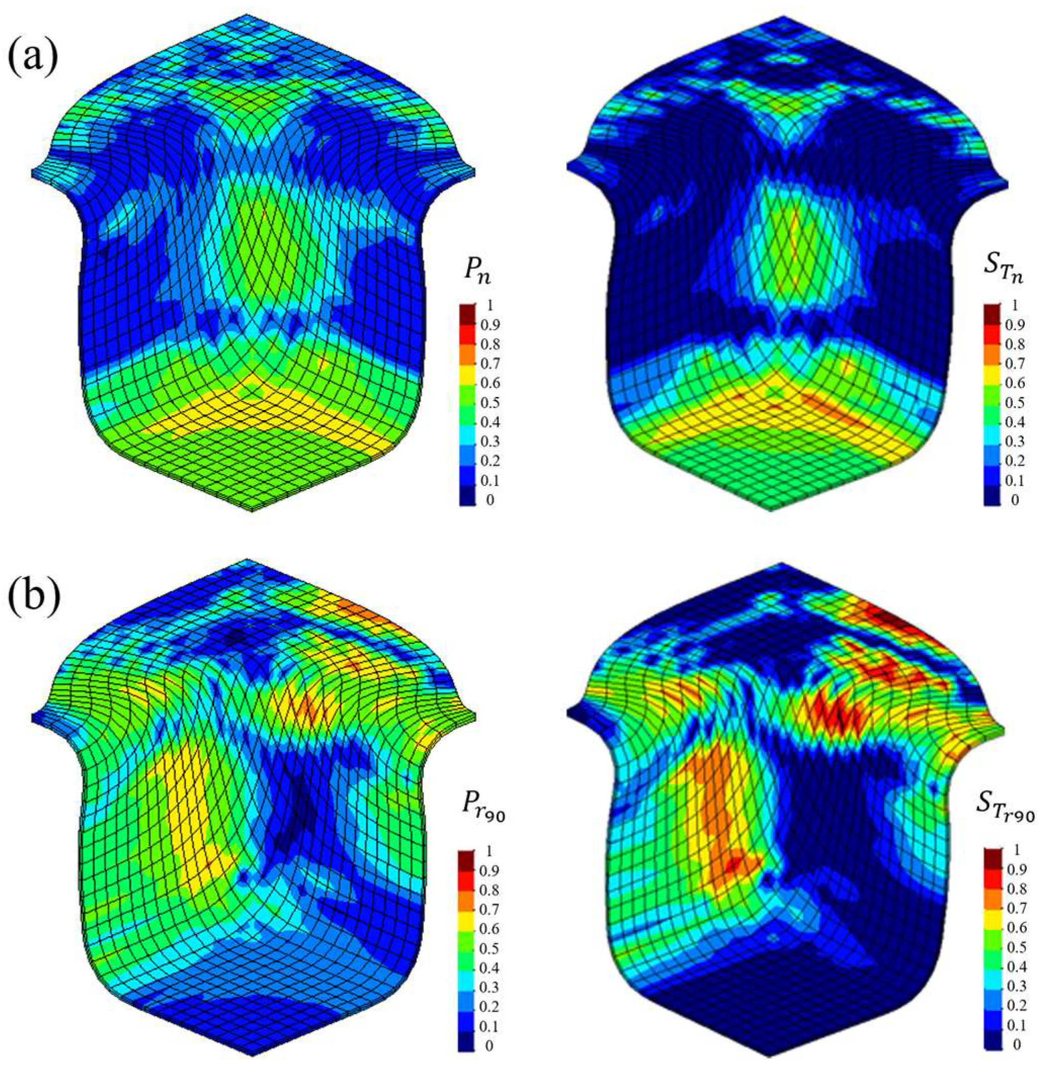
3.3. Sensitivity Indices per Region of the Square Cup
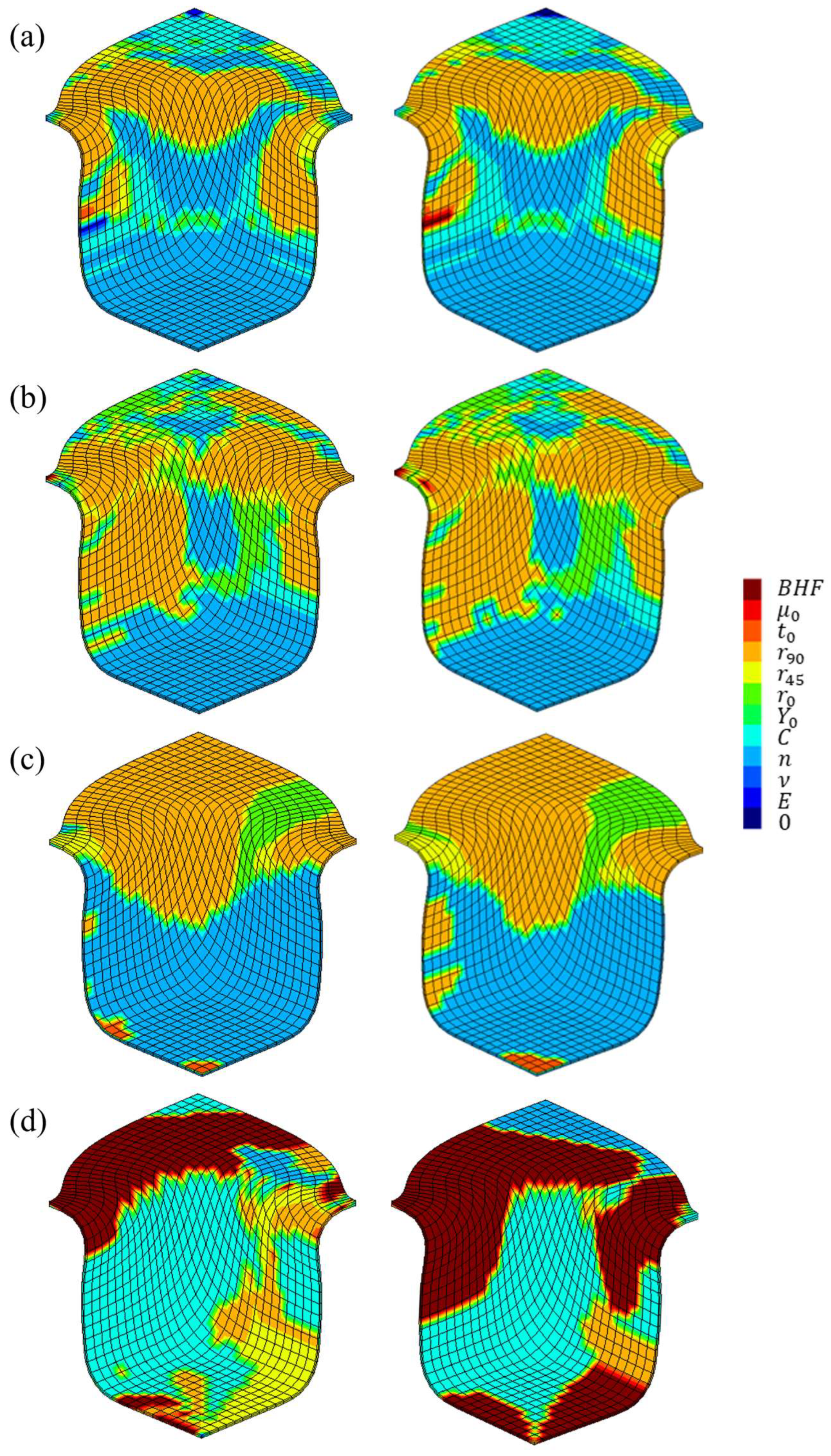
3.4. Maximum Sensitivity Indices per Region of the Square Cup
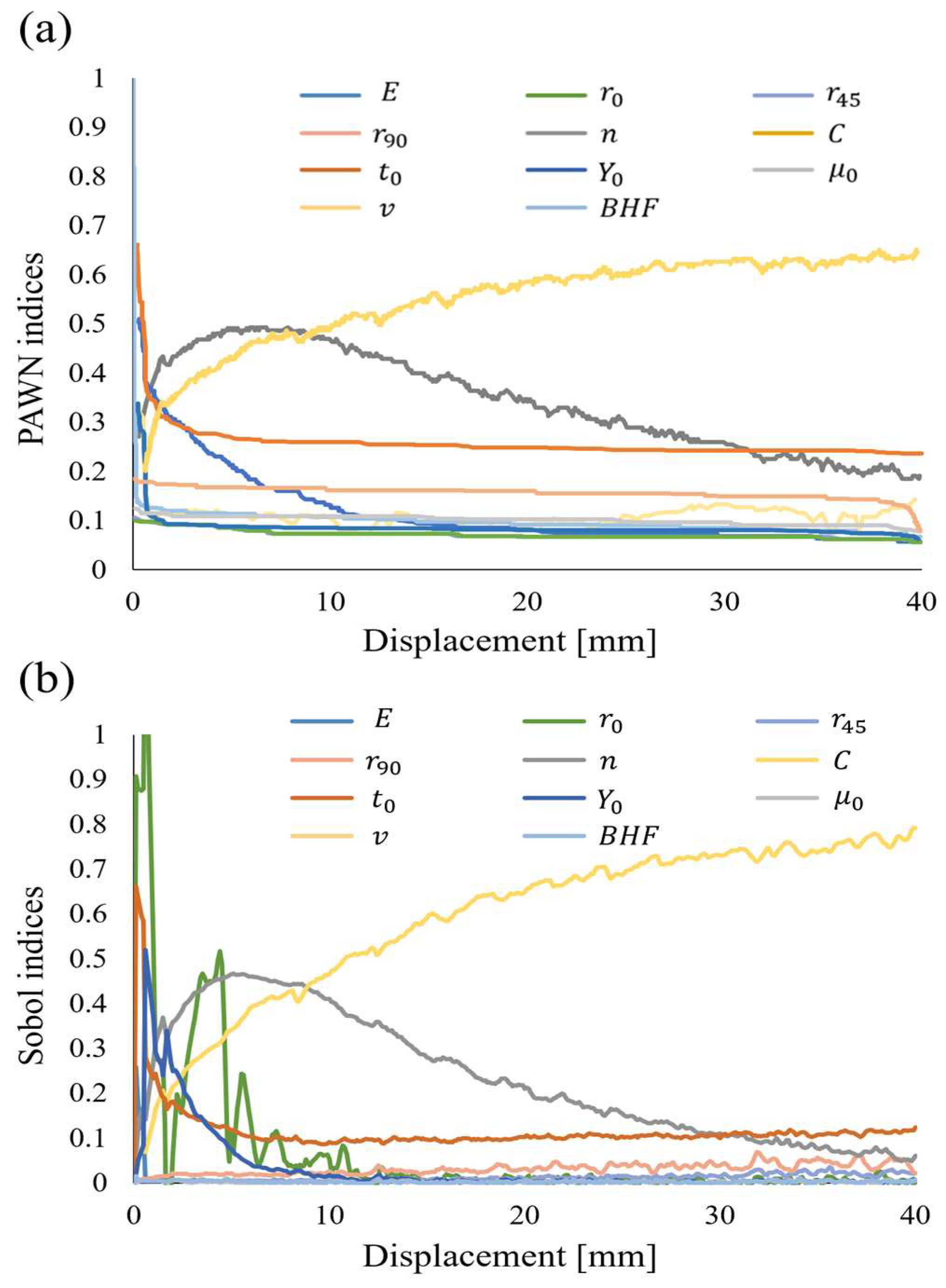
3.5. Evolution of Sensitivity Indices for the Punch Force
4. Conclusions
Author Contributions
Funding
Data Availability Statement
Conflicts of Interest
References
- Gronostajski, Z.; Pater, Z.; Madej, L.; Gontarz, A.; Lisiecki, L.; Łukaszek-Sołek, A.; Łuksza, J.; Mróz, S.; Muskalski, Z.; Muzykiewicz, W.; et al. Recent Development Trends in Metal Forming. Arch. Civ. Mech. Eng. 2019, 19, 898–941. [Google Scholar] [CrossRef]
- de Souza, T.; Rolfe, B. Multivariate Modelling of Variability in Sheet Metal Forming. J. Mater. Process. Technol. 2008, 203, 1–12. [Google Scholar] [CrossRef]
- Lim, Y.; Venugopal, R.; Ulsoy, A.G. Advances in the Control of Sheet Metal Forming. IFAC Proc. Vol. 2008, 41, 1875–1883. [Google Scholar] [CrossRef]
- Hazra, S.; Williams, D.; Roy, R.; Aylmore, R.; Smith, A. Effect of Material and Process Variability on the Formability of Aluminium Alloys. J. Mater. Process. Technol. 2011, 211, 1516–1526. [Google Scholar] [CrossRef]
- Han, S.S. The Influence of Tool Geometry on Friction Behavior in Sheet Metal Forming. J. Mater. Process. Technol. 1997, 63, 129–133. [Google Scholar] [CrossRef]
- Majeske, K.D.; Hammett, P.C. Identifying Sources of Variation in Sheet Metal Stamping. Int. J. Flex. Manuf. Syst. 2003, 15, 5–18. [Google Scholar] [CrossRef]
- Li, Y.Q.; Cui, Z.S.; Ruan, X.Y.; Zhang, D.J. Application of Six Sigma Robust Optimization in Sheet Metal Forming. In Proceedings of the 6th International Conference and Workshop on Numerical Simulation of 3D Sheet Metal Forming Process, Detroit, MI, USA, 15–19 August 2005; Volume 778 A, pp. 819–824. [Google Scholar]
- Faes, M.; Van Doninck, B.; Imholz, M.; Moens, D. Product Reliability Optimization under Plate Sheet Forming Process Variability. In Proceedings of the 8th International Workshop on Reliable Computing, Liverpool, UK, 16–18 July 2018. [Google Scholar]
- Ledoux, Y.; Sergent, A.; Arrieux, R. Impact of the Material Variability on the Stamping Process: Numerical and Analytical Analysis. In AIP Conference Proceedings, Proceedings of the 9th International Conference on Numerical Methods in Industrial Forming Processes, Porto, Portugal, 17–21 June 2007; AIP Publishing: New York, NY, USA, 2007; Volume 908, pp. 1213–1218. [Google Scholar]
- Marretta, L.; Di Lorenzo, R. Influence of Material Properties Variability on Springback and Thinning in Sheet Stamping Processes: A Stochastic Analysis. Int. J. Adv. Manuf. Technol. 2010, 51, 117–134. [Google Scholar] [CrossRef]
- Strano, M. A Technique for FEM Optimization under Reliability Constraint of Process Variables in Sheet Metal Forming. Int. J. Mater. Form. 2008, 1, 13–20. [Google Scholar] [CrossRef]
- Huang, C.; Radi, B.; Hami, A. El Uncertainty Analysis of Deep Drawing Using Surrogate Model Based Probabilistic Method. Int. J. Adv. Manuf. Technol. 2016, 86, 3229–3240. [Google Scholar] [CrossRef]
- Arnst, M.; Ponthot, J.P.; Boman, R. Comparison of Stochastic and Interval Methods for Uncertainty Quantification of Metal Forming Processes. Comptes Rendus-Mec. 2018, 346, 634–646. [Google Scholar] [CrossRef]
- Shahi, V.J.; Masoumi, A.; Franciosa, P.; Ceglarek, D. Quality-Driven Optimization of Assembly Line Configuration for Multi-Station Assembly Systems with Compliant Non-Ideal Sheet Metal Parts. Procedia CIRP 2018, 75, 45–50. [Google Scholar] [CrossRef]
- Dwivedy, M.; Kalluri, V. The Effect of Process Parameters on Forming Forces in Single Point Incremental Forming. Procedia Manuf. 2019, 29, 120–128. [Google Scholar] [CrossRef]
- Prates, P.A.; Adaixo, A.S.; Oliveira, M.C.; Fernandes, J.V. Numerical Study on the Effect of Mechanical Properties Variability in Sheet Metal Forming Processes. Int. J. Adv. Manuf. Technol. 2018, 96, 561–580. [Google Scholar] [CrossRef]
- Marques, A.E.; Prates, P.A.; Pereira, A.F.G.; Oliveira, M.C.; Fernandes, J.V.; Ribeiro, B.M. Performance Comparison of Parametric and Non-Parametric Regression Models for Uncertainty Analysis of Sheet Metal Forming Processes. Metals 2020, 10, 457. [Google Scholar] [CrossRef]
- Dib, M.A.; Oliveira, N.J.; Marques, A.E.; Oliveira, M.C.; Fernandes, J.V.; Ribeiro, B.M.; Prates, P.A. Single and Ensemble Classifiers for Defect Prediction in Sheet Metal Forming under Variability. Neural Comput. Appl. 2020, 32, 12335–12349. [Google Scholar] [CrossRef]
- Bérend, N.; Le Riche, R. Comparison of Different Global Sensitivity Analysis Methods for Aerospace Vehicle Optimal Design. In Proceedings of the 10th World Congress on Structural and Multidisciplinary Optimization, Orlando, FL, USA, 19–24 May 2013. [Google Scholar]
- Pianosi, F.; Wagener, T. A Simple and Efficient Method for Global Sensitivity Analysis Based On cumulative Distribution Functions. Environ. Model. Softw. 2015, 67, 1–11. [Google Scholar] [CrossRef]
- Pianosi, F.; Wagener, T. Distribution-Based Sensitivity Analysis from a Generic Input-Output Sample. Environ. Model. Softw. 2018, 108, 197–207. [Google Scholar] [CrossRef]
- Puy, A.; Lo Piano, S.; Saltelli, A. A Sensitivity Analysis of the PAWN Sensitivity Index. Environ. Model. Softw. 2020, 127, 104679. [Google Scholar] [CrossRef]
- Pereira, A.F.G.; Ruivo, M.F.; Oliveira, M.C.; Fernandes, J.V.; Prates, P.A. Numerical Study of the Square Cup Stamping Process: A Stochastic Analysis. In Proceedings of the ESAFORM 2021—24th International Conference on Material Forming, Liege, Belgium, 16–14 April 2021; PoPuPS (University of Liege Library): Liège, Belgium, 2021. [Google Scholar]
- Bayraktar, E.; Altintaş, S. Square Cup Deep Drawing Experiments. In Proceedings of the 2nd International Conference Numerical Simulation of 3-D Sheet Metal Forming Processes, NUMISHEET ’93, Isehara, Japan, 31 August–2 September 1993; p. 441. [Google Scholar]
- Neto, D.M.; Oliveira, M.C.; Menezes, L.F. Surface Smoothing Procedures in Computational Contact Mechanics. Arch. Comput. Methods Eng. 2017, 24, 37–87. [Google Scholar] [CrossRef]
- Menezes, L.F.; Teodosiu, C. Three-Dimensional Numerical Simulation of the Deep-Drawing Process Using Solid Finite Elements. J. Mater. Process. Technol. 2000, 97, 100–106. [Google Scholar] [CrossRef]
- Hill, R. A Theory of the Yielding and Plastic Flow of Anisotropic Metals. Proc. R. Soc. London Ser. A Math. Phys. Sci. 1948, 193, 281–297. [Google Scholar]
- Swift, H.W. Plastic Instability under Plane Stress. J. Mech. Phys. Solids 1952, 1, 1–18. [Google Scholar] [CrossRef]
- Sobol’, I.M. On the Distribution of Points in a Cube and the Approximate Evaluation of Integrals. USSR Comput. Math. Math. Phys. 1967, 7, 86–112. [Google Scholar] [CrossRef]
- Saltelli, A.; Ratto, M.; Andres, T.; Campolongo, F.; Cariboni, J.; Gatelli, D.; Saisana, M.; Tarantola, S. Global Sensitivity Analysis. The Primer; John Wiley & Sons: Hoboken, NJ, USA, 2008. [Google Scholar] [CrossRef]


Disclaimer/Publisher’s Note: The statements, opinions and data contained in all publications are solely those of the individual author(s) and contributor(s) and not of MDPI and/or the editor(s). MDPI and/or the editor(s) disclaim responsibility for any injury to people or property resulting from any ideas, methods, instructions or products referred to in the content. |
© 2024 by the authors. Licensee MDPI, Basel, Switzerland. This article is an open access article distributed under the terms and conditions of the Creative Commons Attribution (CC BY) license (https://creativecommons.org/licenses/by/4.0/).
Share and Cite
Parreira, T.G.; Rodrigues, D.C.; Oliveira, M.C.; Sakharova, N.A.; Prates, P.A.; Pereira, A.F.G. Sensitivity Analysis of the Square Cup Forming Process Using PAWN and Sobol Indices. Metals 2024, 14, 432. https://doi.org/10.3390/met14040432
Parreira TG, Rodrigues DC, Oliveira MC, Sakharova NA, Prates PA, Pereira AFG. Sensitivity Analysis of the Square Cup Forming Process Using PAWN and Sobol Indices. Metals. 2024; 14(4):432. https://doi.org/10.3390/met14040432
Chicago/Turabian StyleParreira, Tomás G., Diogo C. Rodrigues, Marta C. Oliveira, Nataliya A. Sakharova, Pedro A. Prates, and André F. G. Pereira. 2024. "Sensitivity Analysis of the Square Cup Forming Process Using PAWN and Sobol Indices" Metals 14, no. 4: 432. https://doi.org/10.3390/met14040432
APA StyleParreira, T. G., Rodrigues, D. C., Oliveira, M. C., Sakharova, N. A., Prates, P. A., & Pereira, A. F. G. (2024). Sensitivity Analysis of the Square Cup Forming Process Using PAWN and Sobol Indices. Metals, 14(4), 432. https://doi.org/10.3390/met14040432