Abstract
Aiming at ensuring the quality of the product and reducing the cost of steel manufacturing, an increasing number of studies have been developing nonlinear regression models for the prediction of the mechanical properties of steel rebars using machine learning techniques. Bearing this in mind, we revisit this problem by developing a design methodology that amalgamates two powerful concepts in parsimonious model building: (i) sparsity, in the sense that few support vectors are required for building the predictive model, and () locality, in the sense that simpler models can be fitted to smaller data partitions. In this regard, two regression models based on the Least Squares Support Vector Regression (LSSVR) model are developed. The first one is an improved sparse version of the one introduced in a previous work. The second one is a novel local LSSVR-based regression model. The task of interest is the prediction of four output variables (the mechanical properties YS, UTS, UTS/YS, and PE) based on information about its chemical composition (12 variables) and the parameters of the heat treatment rolling (6 variables). The proposed LSSVR-based regression models are evaluated using real-world data collected from steel rebar manufacturing and compared with the global LSSVR model. The local sparse LSSVR approach was able to consistently outperform the standard single regression model approach in the task of interest, achieving improvements in the average from previous studies: 5.04% for UTS, 5.19% for YS, 1.96% for UTS/YS, and 3.41% for PE. Furthermore, the sparsification of the dataset and the local modeling approach significantly reduce the number of SV operations on average, utilizing 34.0% of the total SVs available for UTS estimation, 44.0% for YS, 31.3% for UTS/YS, and 32.8% for PE.
1. Introduction
The prediction of mechanical properties in steel manufacturing holds paramount importance for the steel industry, ensuring both cost-effectiveness and quality. In particular, hot-rolled steel rebars, also known as reinforcing bars (or simply rebars), have been primarily used in reinforcing concrete structures, providing strength and durability to buildings, bridges, and other infrastructure projects. Among the key mechanical properties of interest to steel rebars, one can mention yield strength (YS), ultimate tensile strength (UTS), the UTS/YS ratio, and percent elongation (PE) [,]. The quantities YS and UTS are important performance indicators of materials under load conditions, representing, respectively, the starting point of permanent deformation and the maximum load the material can withstand before failure. The UTS/YS ratio is a material’s ductility measure, while PE is an indicator of the material’s ability to deform without fracturing [,].
It is widely known that the aforementioned mechanical properties of steel rebars are heavily dependent on their chemical composition and on parameters related to production processes [,]. However, these properties are still determined through costly and time-consuming laboratory tests on samples taken from the batch produced. Bearing this in mind, many authors have been using data-driven alternatives to anticipate (or predict) such mechanical properties in an attempt to optimize the manufacturing process. Due to the complexity of the task, these alternatives consist basically of fitting a nonlinear regression model to the available data, using as inputs information from chemical composition and parameters from the production process (e.g., from heat treatment rolling) and as outputs one or more of the quantities of interest (US, UTS, and PE).
Machine learning models have often been chosen for building nonlinear regression models to predict the mechanical properties of products in the steelmaking industry. Examples that are worth mentioning are found in the manufacturing of hot-rolled steel plates [], cold-rolled galvanized steel coils [], interstitial-free steels [], hot-rolled steel rebars [,], and steelmaking in general [,,,]. One of the first successful applications of machine-learning-based regression models to the prediction of the mechanical properties of steel is reported in []. In this work, the authors used support vector regression (SVR) with 29 inputs (19 extracted from chemical composition and 10 from hot-rolling parameters) to predict the mechanical properties of hot-rolled plain carbon steel Q235B, quantified as three output variables (YS, UTS, and PE). Using data collected from the supervisor of the hot-rolling process, the SVR-based approach achieved good performance, according to the authors.
The authors in [] introduced a one-hidden-layered multilayer perceptron (MLP) to model and optimize the chemical composition of a steel bar with the goal of predicting its mechanical properties, considering UTS and YS as output variables. This MLP-based regression model was optimized via particle swarm optimization (PSO) in order to exploit better solutions in the search space through iterations. According to the authors, the obtained results were consistent with the actual data. Following a similar paradigm, a single-hidden-layered MLP-based regression model was also developed in [] to predict the mechanical properties of a coil, namely, YS and UTS, from its chemical composition, thickness, width, and key galvanizing process parameters, resulting in a total of 23 input variables. An online quality monitoring system was developed with the goal of monitoring the predicted mechanical properties and process parameters of a galvanized coil, helping the quality team in decision making.
The predictive model developed in [] is built on 18 inputs derived from the chemical composition (12 inputs) and heat treatment (6 inputs) of steel rebars. The methods employed include multiple linear regression and a two-hidden-layered MLP whose goal is to predict the mechanical properties of steel rebars, namely, YS, UTS (or alternatively, the ratio UTS/YS), and PE. The best performance, measured by R2 values, was obtained by the MLP-based regression model. A two-hidden-layered MLP with 27 inputs is designed in [] to predict the mechanical properties (YS, UTS, EL, and impact energy) of industrial steel plates based on the process parameters and the composition of the raw steel. The authors applied this model online to a real steel manufacturing plant.
Four machine learning methods were evaluated in [] in the task of predicting the hot ductility of cast steel from chemical composition and thermal conditions. A single-hidden-layered MLP achieved the best performance in comparison with random forest, Gaussian process, and SVR. A single-hidden-layered MLP was also used in [] to predict the mechanical properties of ultra-fine-grained Fe-C alloy by fusing the experimental combinations of alloy composition, rolling process parameters, and heat treatment process parameters. In this work, the MLP outperformed the SVR model and an MLP variant trained with a genetic algorithm. In [], the UTS of both non-spliced and spliced bars is predicted using nonlinear regression, ridge regression, and MLP, achieving accurate results. In [], tree-based machine learning techniques, namely, decision trees and random forests, are implemented to analyze the ultimate strain of non-spliced and spliced steel reinforcements, achieving acceptable results. The authors highlight further that the evaluated tree-based regression models were time-saving and cost-effective compared with more complicated, time-consuming, and expensive experimental examinations.
An ELM-based regression model [], a neural network architecture whose input-to-hidden layer weights are randomly sampled and not allowed to be modified during training, was developed in [] to predict the mechanical properties of an aluminum alloy strip. The obtained results show that the proposed ELM-based regression model achieved high accuracy and stability in predicting aluminum alloy strips’ YS, UTS, and PE. The main advantage of the ELM over more traditional machine learning methods, such as the MLP and SVR, relies on the very short time required for training the regression model.
Despite its popularity in machine learning, applications of deep learning (DL) models for predicting the mechanical properties of steel are still in their infancy. We hypothesize that this occurs because of the type of input information. Most DL architectures, especially those based on convolutional neural networks (CNNs), require images as inputs. In visual inspection tasks, where image acquisition is usual, the application of CNNs is dominant nowadays. For example, in [], a deep learning approach based on a YOLOv3 detector [] is used for automatic steel bar detection and counting through images. Thus, to use a CNN, it is necessary to convert the production data into 2D data images, as performed in [], for predicting the mechanical properties of hot-rolled steel using chemical composition and process parameters.
Of particular interest to the current paper is the work of Murta et al. [], who used the Least Squares Support Vector Regression (LSSVR) [] model for predicting the mechanical properties of steel rebar. It was built on 18 inputs and 4 outputs (YS, UTS, UTS/YS ratio, and PE), with the LSSVR model outperforming the MLP-based regression model developed in [] on the same dataset. Motivated by this result, we revisit the LSSVR model with the goal of improving its performance on the prediction task of interest. In this context, sparsification approaches are highly important when dealing with support-vector-based models, as the computational complexity typically scales cubically with the size of the training set []. For this purpose, we initially evaluate vector quantization methods [,] and then introduce a novel approach for using the approximate linear dependence (ALD) method [] in the sparsification of the LSSVR model for non-temporal data. Additionally, we make use of the local regression paradigm to develop a novel approach for predicting the mechanical properties of steel rebars. Unlike the single regression model approach, local regression modeling divides the dataset into smaller regions and constructs a separate regression model for each region. This approach has been successfully used in various regression problems, such as identifying failure modes of reinforced concrete shear walls [], composite autoclave manufacturing [], and polyethylene production [].
In summary, in the current paper, we aim at building two LSSVR-based regression models that can be used before the actual manufacturing process takes place so that the mechanical properties of the produced steel rebar resemble the most predicted ones. The main contributions, from the machine learning perspective, consist in the development of two sparse LSSVR-based models, one based on the global modeling paradigm and the other based on the local modeling paradigm. From the perspective of process engineering, the proposed regression models can be used to experiment with different values of the 18 input variables and foresee the resulting four mechanical properties of the steel rebars. It may turn out to be important in the statistical quality control of the produced steel rebars. The fitted regression model can also be used for online (or offline) process monitoring. That is, it can reveal problems in the actual process if there is any disparity between the actual and predicted mechanical properties of the steel rebar. From the perspective of materials engineering, as the regression model can be understood as an emulator of a complex production process, the model can be used to investigate the effect of each input variable on the mechanical properties of the steel produced. Ultimately, the model can be used for teaching purposes.
The remainder of the paper is organized in the following sections: In Section 2, we provide details on the materials and methods employed in this study. This section encompasses a description of the experimental setup, the materials utilized, and the procedures followed to ensure the reliability and reproducibility of the results. The results are presented and discussed in Section 3. We conclude the paper by presenting a summary of the contributions and achieved results in Section 4.
2. Materials and Methods
In this section, we provide a general understanding of the materials and methods utilized in this study. Section 2.1 briefly reviews the steel rebar manufacturing dataset and its origins from the production data. Section 2.2 describes the basics of the LSSVR model. Section 2.3 introduces the support vector reduction methods used by the LSSVR-based regression models. In Section 2.4, we present the fundamentals of cluster-based local modeling. Section 2.5 details the methodology of computer simulations.
2.1. Steel Rebar Manufacturing Dataset
The steel rebar manufacturing dataset encompasses two distinct sets of input variables, totaling 18 inputs, which are used for building the regression models (see Figure 1). The first set comprises six process parameters, while the other contains twelve parameters related to the steel’s chemical composition. The 6 inputs of the first group are the cross-sectional area of the steel bar after rolling, the finishing rolling temperature, the initial and final temperatures of heat treatment, and the pressure and flow of the heat treatment water.
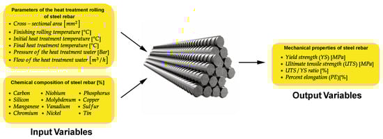
Figure 1.
Illustration highlighting the input and output variables used for building the regression models in this paper. All the 18 input variables are used by the steel company that provided the dataset in its steel rebar manufacturing process.
Table 1 provides information on the range of hot-rolling and heat treatment parameters applied. The cross-sectional area of the steel bar is related to the force required to reduce its dimensions in the rolling process and the temperature gradient of the heat treatment. The final rolling temperature and the initial and final temperatures of heat treatment are related to the steel’s microstructure. The pressure of the heat treatment water affects the temperature gradient within the core and the thickness of the outer martensite layer produced. The cross-sectional areas of the steel bar after rolling correspond to 50 mm2, 71 mm2, 113 mm2, 129 mm2, and 199 mm2. The studied rebar diameters were 8 mm, 10 mm, 12 mm, 1/2″ (12.7 mm), 3/8 (9.525 mm), and 5/8 (15.875 mm).

Table 1.
Parameters of the heat treatment rolling of steel rebar.
The remaining input variables are related to the concentration of carbon, niobium, phosphorus, silicon, molybdenum, copper, manganese, vanadium, sulfur, chromium, nickel, and tin, which are elements that can influence the mechanical properties of alloys. Table 2 presents a statistical description of the chemical composition of the steel dataset used in this research. These 18 input variables are used by the kernel regression models evaluated in this paper to predict the following output variables: YS, UTS, UTS/YS ratio, and PE, presented in Table 3. Finally, altogether, the dataset comprises 1300 instances.
Table 2.
Input variables related to chemical composition [%].
Table 3.
Output mechanical properties of the rebar by the models.
It should be mentioned that we are handling a very specific problem, which is the prediction (from the point of view of a regression task) of the macroscale properties of rebar steel based on information about its chemical composition (12 variables) and parameters of the heat treatment rolling (6 variables). The dataset was kindly provided by a Brazilian steel multinational, which owns a patent on the steel bar manufacturing process that originated the dataset. The heat treatment used is referred to by the company as THERMEX, which is commonly referred to in the existing literature as Tempcore Process [].
2.2. Least Squares Support Vector Regression
Building a regression model from data presupposes the availability of a group of tuples (samples) , where are the prediction variables and are the corresponding observed outputs. Without loss of generality, considering a single output () to describe an approach for kernel-based methods, a regression model can be expressed as follows:
where is a non-linear mapping into a high-dimensional space H, is the corresponding parameter vector, and is the bias term.
Specifically, the LSSVR model’s parameters are estimated by minimizing the following loss function:
subject to the following:
where , is the error associated with the n-th sample, and , an hyperparameter, is a regularization constant to be evaluated considering both the training error and the smoothness of the regression function.
This optimization problem has its formulation in the dual space written as the following Lagrangian:
where represents the vector of Lagrange multipliers. The solution to (4) can be obtained through the Karush–Kuhn–Tucker optimality conditions, rewriting the problem into the following linear system:
where , is a vector of 1’s, is an identity matrix, and is the kernel matrix with elements . One way to emulate the inner product of a nonlinear mapping into a high-dimensional space is by using the kernel trick, where a function satisfying the Mercer conditions (sufficient conditions to ensure that a matrix is symmetric and positive definite.) is used, such as the Gaussian function chosen for the experiments in this work, given by the following:
where is the kernel function, is the Euclidean norm, and denotes the width of the Gaussian function (a hyperparameter to be fine-tuned). With this solution, the regression model is expressed as follows:
Unlike the SVR model, which produces a sparse solution in terms of constructing the model using only a few vectors from the training set, henceforth named support vectors (SVs), the LSSVR model often utilizes all available data. In other words, the entire set of SVs, denoted by , must be stored to build the predictive model. Thus, techniques for reducing the number of SVs are employed to simplify the internal structure of the LSSVR [,]. In the next section, some of these techniques are presented for performance comparison.
2.3. Support Vector Reduction Methods
To reduce the number of SVs in the LSSVR, four sparsification procedures are employed. The first method involves a straightforward random selection of SVs from the training data, serving as a baseline to evaluate the performance of other approaches.
In the second approach, the k-means algorithm [], which is a vector quantization (VQ) technique commonly employed for data volume reduction [], is used. In this context, the goal is to represent an original dataset by a reduced set formed by prototypes, without significant loss of information. Therefore, the selection of SVs is based on dissimilarity, as each prototype replaces similar data points in the construction of the sparse model.
However, the k-means algorithm may be sensitive to outlying samples. Bearing this in mind, the third method applied is the k-medoids algorithm [] for VQ, which is a robust approach when the prototypes computed by the mean of points are not adequate representations of the dataset. Finally, the fourth approach is a proposed modification of the ALD method, ALD for Pruning (ALD4P), which aims to find a subset of the most independent SVs given the non-linear mapping induced by a kernel function (in this work, the Gaussian function).
2.3.1. K-Means for Vector Quantization
In this work, as the k-means is an unsupervised algorithm that uses just the inputs of a dataset in order to divide it into K partitions, this algorithm is applied to our adapted dataset with concatenated inputs and outputs, i.e., , and we have used the squared Euclidean distance as an objective function, defining the VQ problem as follows:
where is the centroid vector (prototype) of the partition . To achieve this, the algorithm proceeds as follows: In step 1, centroids are randomly initialized from the vectors in the set . In step 2, each vector is then assigned to the nearest centroid , forming the partition . Subsequently, in step 3, each centroid is updated by calculating its new position as the arithmetic mean of the vectors in the partition . Steps 2 and 3 are repeated until there are no changes in the positions of the centroids.
This iterative process optimizes centroid placement to effectively represent the data for clustering analysis. After this process, each centroid is split into input–output pairs: , resulting in a sparse training set .
2.3.2. K-Medoids for Vector Quantization
The k-medoids algorithm replaces the centroid in (8) by the medoid , such that is necessarily a vector from the set . This algorithm follows a series of steps: First, initialize the medoids randomly from the vectors in the set . In step 2, assign each vector to the nearest medoid , forming the partition . In step 3, for each vector belonging to the cluster , calculate the sum of distances between it and the other elements of the partition. In step 4, update each medoid with the vector from its respective partition that has the smallest sum of distances in step 3. Repeat steps 2 to 4 until there are no changes in the medoids.
At the end of this technique, as the k-means, each medoid is split into input–output pairs: , resulting in a sparse training set . However, is not just a representation of the original data.
2.3.3. ALD for Pruning SVs Instead of Inserting Them
In order to sequentially remove samples from a dataset, we introduce a variant of the ALD method that is a widely used sparsification technique for selecting the relevant prototypes of a dataset while support-vector-based models are being trained online []. The proposed variant prunes SVs from a large set of samples instead of inserting them one by one, as is usually the case in the processing of temporal data. Since we are dealing with non-temporal data, the pruning approach fits better with the requirements of the regression task we are dealing with.
Originally, this method works in the following manner: At the training time step t, with N denoting the number of training samples, after having observed training samples, the dictionary is composed of a subset of relevant training inputs . When a new incoming training sample is available, one must test if it should be added or not to the dictionary. In order to do this, it is necessary to estimate a vector of coefficients satisfying the following ALD criterion:
where is the sparsity level parameter. Developing the minimization problem in Equation (9) and using , using the matrix notation, we can write the following:
where , , and , with . Solving (10) leads to the optimal , given by the following:
so that the ALD condition can be rewritten as follows:
If , then the sample must be added to the dictionary, that is, and . However, if , the sample is approximately linearly dependent and must not be added to the dictionary.
However, in this work, we adapted the ALD method to sequentially remove the “most linear dependent sample” from the dataset. First, the dictionary is composed of N samples (all the training dataset). Then, in removing step 1, N values of will be generated by considering a specific removed sample as (see Equations (9)–(12)) and a dictionary composed of the remaining samples. The sample to be removed, in this step, is the one that generates the smaller , as it represents the most linearly dependent sample from the others. In removing step 2, values of will be generated using the resulting dataset from the previous step. This procedure is performed until a maximum number of sequentially removed samples are reached.
Following the description of sparsification techniques to be used for building the LSSVR-based regression models, we will now delve into a novel approach aimed at enhancing local learning capabilities of the LSSVR model.
2.4. Cluster-Based Local Modeling
The local learning paradigm enables model adaptation by capturing various complex and nonlinear relationships in the data variables across different regions of their feature space. Instead of assuming a single global representation, these local models are typically simpler and can interact cooperatively or competitively, providing greater interpretability of the problem and operational flexibility. Moreover, the local approach allows for maintaining or even enhancing prediction accuracy compared with the global model [].
In the context of the local LSSVR model, cluster-based local modeling [] presents an interesting proposal for reducing prediction computational costs. To achieve this, the local model involves partitioning the training dataset based on some locality criterion. In this article, the k-means algorithm is used for clustering the set of input data, , into K partitions, guided by the squared Euclidean distance. For each of these partitions , an LSSVR model is constructed with the following partitioning of the data .
After the training step, the local model outputs can be combined as follows:
where is a weighting function for the local LSSVR outputs . In a winner-takes-all (WTA) approach, only one local model is selected to perform the output prediction. Thus, the algorithm calculates the distances from the input vector of the new sample to each centroid corresponding to the partitions found by the k-means algorithm. In this way, the winning model is the one whose respective centroid is the closest one to the current input vector, defining the weighting function as follows:
In words, the weighting function in Equation (13) is determined after a search for the nearest prototype vector to the current input vector . For the nearest prototype vector, we set . Otherwise, , as shown in Equation (14). This is valid only for hard clustering techniques, such as the k-means algorithm used in this paper. This implies that only a subset of the available SVs are utilized in each prediction by means of a local model. For soft clustering techniques [], such as fuzzy clustering algorithms (not used in the current paper), the weighting factor may assume values between 0 and 1, meaning that the local models may use data samples from neighboring clusters weighted by their membership values.
Based on the theoretical foundations outlined, our methodology translates these principles into a practical nonlinear regression framework. Drawing from insights on LSSVR sparsification techniques, our approach optimizes model performance while reducing its complexity. Additionally, integrating local learning within LSSVR enhances adaptability to data patterns. Subsequent sections detail our step-by-step methodology, bridging theory with application.
2.5. Methodology
In the following experiments, whose MATLAB® (R2023b) codes and datasets are available on GitHub (https://github.com/spiral-ufc/slssvr-rebar, accessed on 5 June 2024), 100 independent realizations are made for each built model. First, the dataset is shuffled 100 times, each one with a specific random seed . The dataset is then divided into two groups: one for training and one for testing. Consequently, the algorithms utilize the same 100 splits across all experiments. Additionally, z-score normalization is applied to both groups using only the training set statistics, and the predicted outputs of the models are denormalized for performance evaluation.
The figure of merit used in order to compare the performances of these new results with the ones in [,] is the coefficient of determination (), given by the following:
where is the number of test samples, is the n-th observed output, is the arithmetic mean of all observed output values from the test set, and is the n-th predicted output.
Hyperparameter tuning is a critical step in building a regression model. In [], the LS-SVMlab Toolbox (version 1.8) [] is used to implement the LSSVR model. In the current version of this toolbox, the hyperparameters are optimized using the Coupled Simulated Annealing (CSA) method and the simplex method. First, the CSA algorithm is responsible for exploring the search space. Then, the simplex method refines the solution, reducing the number of objective function evaluations and improving the solution quality compared with when these algorithms are used separately. Nevertheless, in the experiments conducted in this study, we combined the metaheuristic Particle Swarm Optimization (PSO) [,] with the Nelder–Mead simplex method [,] in a custom implementation of the LSSVR (built from scratch). The goal of implementing our solution is to have more freedom and ease in proposing improvements to the LSSVR model.
In each experiment realization, the hyperparameters of the kernel regression models, namely, the width of the Gaussian function and the regularization constant , are optimized using the joint approach of PSO and simplex algorithms applied to the non-sparse LSSVR. For this optimization, a 10-fold cross-validation is applied to the training dataset, and the mean squared error is used as the cost function. Then, these estimated optimal hyperparameters are applied to all other evaluated models.
More specifically, a global PSO algorithm is constructed with a swarm of five particles with two positions each. The search interval for the two hyperparameters is within . After randomly initializing the swarm, five iterations are computed, and the best result obtained serves as the initial point for the simplex method. The MATLAB® function @fminsearch is employed to exploit the solution found by PSO, with a limit of 100 iterations in case of non-convergence. Figure 2 shows a summary diagram of this first part of the methodology for the experiments.
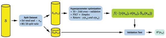
Figure 2.
Summary diagram of the LSSVR hyperparameter optimization.
For support vector reduction methods, an arbitrary number of SVs is imposed on the resulting sparse dataset, and its respective coefficient is calculated. The ALD4P method is implemented from scratch, following the information provided in Section 2.3.3, and utilizes the following hyperparameters: the regularization constant and the width of the Gaussian function (same as the LSSVR model), where SVs are sequentially removed until the desired quantity is reached. As for the VQ methods, the MATLAB® functions @kmeans and @kmedoids are employed, configuring the number of resulting centroids or medoids.
For the local LSSVR approach, the MATLAB® function @kmeans is applied for partitioning the data into subsets for estimating local models. Thus, the performance of the local LSSVR is evaluated with the increase in its local models. Figure 3 provides a general illustration of the experiments conducted in this study.
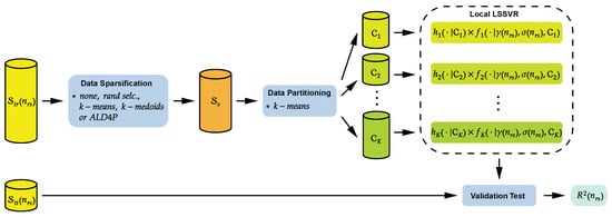
Figure 3.
Summary diagram of computational experiments.
3. Results and Discussions
In this section, we report and discuss the results obtained by applying the kernel regression models and sparsification techniques previously described to predict the mechanical properties of steel rebars. We evaluate the performance of the models for the four studied properties.
3.1. Impact of Varying the Percentage of Training Data on the Accuracy Using the LSSVR Model
To assess the impact of varying the percentage of training data on the accuracy of the test dataset using the LSSVR model, we conducted several trials with different training–testing splits, summarized in Table 4.
Table 4.
Performance comparison for different training and testing splits for the LSSVR in terms of mean and standard deviation of .
Our analysis indicates that, while the test accuracy varies with different splits, a closer look at the results reveals that the first three splitting ratios (50–50%, 60–40%, 70–30%) did not lead to acceptable performances; that is, for all output variables. As expected, the best performance was achieved with the 90–10% ratio at the expense of ending with just a few testing samples, which we believe is not representative of the process. Thus, we judged the 80–20% ratio to be a fairer trade-off between efficiently solving a complex process engineering problem and obtaining high performance rates for the machine learning model. For the sake of simplicity, we adopted the same ratio for building the proposed local LSSVR-based regression models.
3.2. About the Improvement of LSSVR Model Results
In comparison with the results in [], where an LSSVR model is employed with the same dataset, the current study achieves superior results in average with all the data. The improvements obtained for each output are approximately in the average (from 0.7989 to 0.8392) for UTS, (from 0.7389 to 0.7773) for YS, (from 0.8603 to 0.8772) for UTS/YS, and (from 0.6883 to 0.7118) for PE. This improvement in the results of the global LSSVR model is due to a change in hyperparameter optimization methodology. In contrast with the approach in [], where only of the training dataset was utilized for this task, we now employ the entire training dataset. However, this leads to an increase in computational cost during training, justified by the enhancement in model estimation performance.
Another key aspect highlighted in [] is the implementation of a sparsification procedure, where the resulting model utilizes (899) of the available SVs for the UTS output, (906) of the SVs for YS, (889) of the SVs for UTS/YS, and (895) of the SVs for PE. In this paper, we subsequently report on the efforts made in sparsifying the LSSVR model.
Table 5 presents these average values of , as well as their respective standard deviations, and the percentage of the average number of operations with the SVs required for a prediction during the validation testing of the models.
Table 5.
Comparison of performances of evaluated regression models in terms of mean and standard deviation of .
3.3. About the Sparsification of the LSSVR Model
Throughout the analysis of sparsification methods for the LSSVR model, a deliberate choice is made to decrease the number of SVs while upholding performance standards equivalent to those of the full set of SVs. In this sense, a continuous and dashed black line is plotted to represent the values of the non-sparse LSSVR model in terms of average and standard deviation of , respectively, in the performance comparison figures of these methods for the four predicted outputs (Figure 4, Figure 5, Figure 6 and Figure 7). Additionally, an error bar in green is generated to indicate the performance of the random removal of SVs from the model in these plots, i.e., an SV removal without a criterion for a contrast with the evaluated approaches: k-means, k-medoids, and the proposed ALD4P.
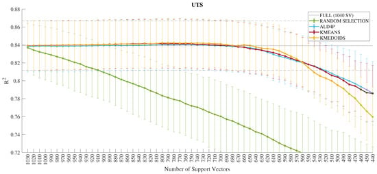
Figure 4.
Performance in of the dimensionality reduction techniques for the UTS output.
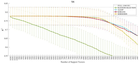
Figure 5.
Performance in of the dimensionality reduction techniques for the YS output.
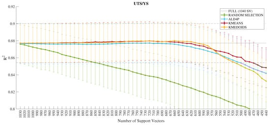
Figure 6.
Performance in of the dimensionality reduction techniques for the UTS/YS ratio output.
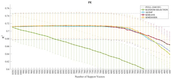
Figure 7.
Performance in of the dimensionality reduction techniques for the PE output.
In a general analysis of the four studied properties, the methodologies present similar performances until there is a degradation of results. Thus, the choice of the winning method is based on the evaluation of other criteria, such as memory for model storage and computational complexity. Regarding memory, the k-means algorithm has the disadvantage of having prototypes instead of real data. Consequently, the four models created cannot share their SVs.
Considering the sparsification methods that select the SVs, the ALD4P method presents a slight numerical disadvantage in the results and is an algorithm with superior complexity compared with the others tested. Therefore, the k-medoids algorithm is chosen to make the LSSVR model more efficient in predicting mechanical properties.
Moving on to an individual evaluation of the models for each output, the error bar of the k-medoids algorithm, in yellow color shown in Figure 4, for the UTS output indicates a quantity of (660) of the SVs without performance loss. In Figure 5, the indication for the YS output is (850) of the SVs. Furthermore, in Figure 6, the indication for the UTS/YS output is (610) of the SVs. Finally, the indication for the PE output is (640) of the SVs, as demonstrated in Figure 7. The proposed sparsifications with their respective values are summarized in Table 5 for the sparse LSSVR (SLSSVR) model.
3.4. About the Local Sparse LSSVR Model
Continuing with the aim of developing a more efficient model, the results of the proposed local LSSVR model in this article are presented. Thus, the partitioning by the k-means algorithm of the SVs into 2 to 10 clusters is verified for all data and for the resulting sparsification of VQ by the k-medoids algorithm.
In Figure 8, the values in relation to the increase in data partitions are shown, in other words, the number of local models that form the local LSSVR model. It is noticed that the error bars between using the complete dataset and the sparse one are practically overlapped, allowing for the choice of partitioning of the selected SVs of the SLSSVR model.
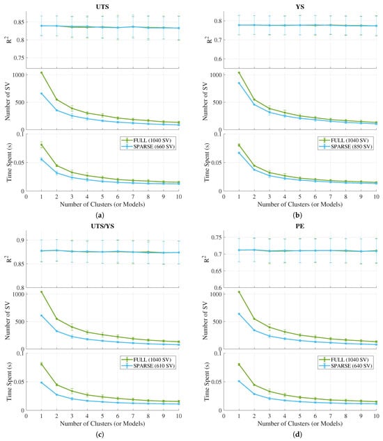
Figure 8.
Performance of the local models along with the respective quantities of SVs used and the time spent during the output prediction of (a) UTS, (b) YS, (c) UTS/YS, and (d) PE.
Furthermore, the study observes the number of SVs utilized and the time required for model prediction during testing. Utilizing only a subset of SVs in calculating the predicted output proves to be an efficient approach, saving computational costs.
Observations reveal that the increase in the number of local models has minimal adverse effects on the values for the four analyzed outputs. This is elucidated in Table 5, which provides numerical results for local SLSSVR models employing two (2L-SLSSVR) and ten local models (10L-SLSSVR).
It is worth pointing that the 2L-SLSSVR model demonstrated no degradation in performance across any of the four predicted outputs; instead, it outperformed the other models. Furthermore, it exhibited a significant average reduction in the number of SVs used during operation. Specifically, it utilized approximately (353) of the SVs for UTS estimation, (457) for YS, (325) for UTS/YS, and (341) for PE during operation. In the case of the 10L-SLSSVR model, it utilized only (86) of the SVs for UTS estimation, (107) for YS, (78) for UTS/YS, and (81) for PE during operation. However, a slight reduction in the model’s performance is already noticeable. Finally, the best result found in this study is that of 2L-SLSSVR in terms of performance, which surpasses the other techniques tested up to that point and summarized in Table 6.
Table 6.
Performance comparison for different machine learning techniques tested in terms of mean and standard deviation of for the steel rebar dataset up to now.
4. Conclusions
In this article, we reported the results of experiments carried out to evaluate possible strategies to enhance the performance of LSSVR models, as reported in previous works, given the significance of their application in metallurgy/steelmaking. The importance of optimizing hyperparameters during training to improve model performance is noted. Additionally, a successful sparsification technique via vector quantization is presented with the k-medoids algorithm, which selects informative samples, reducing the original training dataset without performance loss.
The local modeling approach emerges as a way to make the regression model highly efficient in prediction by using only representative SVs from the cluster to which the test sample belongs, thus reducing the number of operations required for estimation. It showcased a substantial average reduction SV operation: 34.0% of the SVs for UTS estimation, 44.0% for YS, 31.3% for UTS/YS, and 32.8% for PE. Furthermore, the local sparse LSSVR model is introduced as the new state of the art for the Steel Rebar Manufacturing Dataset, achieving the best results so far and suggesting that sparsification and local modeling techniques can be used concurrently without affecting the regression model’s performance.
The enhancement in model prediction reinforces that the chemical composition and thermal treatment parameters in this dataset can be used to predict the four main mechanical properties of steel. The improvements obtained are approximately 5.04% in the average for UTS, 5.19% for YS, 1.96% for UTS/YS, and 3.41% for PE, motivating the application of new techniques in this dataset to surpass the results presented in this study in future works. The raw data supporting the conclusions of this article will be made available by the authors on request.
Possible future works could explore the following research directions: (i) execution of a comprehensive sensitivity analysis on the LSSVR-based regression models in order to understand how each input feature affects the prediction of the mechanical properties, () development of deep learning architectures for the prediction of the mechanical properties of steel rebars, () development of local modeling techniques based on soft clustering, and () investigation of the performance of the regression models proposed in this paper in other datasets within the metallurgy and steel manufacturing domain could provide valuable insights and extend the applicability of these methods.
Furthermore, comparative studies with other regression models and ensemble techniques could be conducted to assess the effectiveness and robustness of the proposed approach in different scenarios. Lastly, exploring the integration of domain knowledge or expert insights into the modeling process could lead to more accurate predictions and a better understanding of the underlying factors influencing steel mechanical properties.
Author Contributions
Conceptualization, R.B. and G.A.B.; methodology, R.B., G.A.B., D.N.C., E.P.d.M. and R.H.F.M.; software, R.B. and D.N.C.; validation, G.A.B. and E.P.d.M.; investigation, R.B., G.A.B., D.N.C., E.P.d.M. and R.H.F.M.; resources, E.P.d.M. and R.H.F.M.; data curation, E.P.d.M. and R.H.F.M.; writing—original draft preparation, R.B.; writing—review and editing, G.A.B., D.N.C. and E.P.d.M.; visualization, E.P.d.M. and R.H.F.M.; supervision, G.A.B. All authors have read and agreed to the published version of the manuscript.
Funding
This study was financed by the Fundação Cearense de Apoio ao Desenvolvimento Científico e Tecnológico (FUNCAP), grant no. PS10186-00103.01.00/21. The authors also thank the Conselho Nacional de Desenvolvimento Científico e Tecnológico (CNPq), grant no. 313251/2023-1, for supporting this research.
Data Availability Statement
The raw data supporting the conclusions of this article will be made available by the authors on request.
Conflicts of Interest
The authors declare no conflicts of interest.
References
- Murta, R.H.F.; de Moura, E.P.; Barreto, G.A. Mechanical properties prediction in rebar using kernel-based regression models. Ironmak. Steelmak. 2022, 49, 1011–1020. [Google Scholar] [CrossRef]
- Murta, R.H.F.; Braga, F.D.; Maia, P.P.N.; Diogenes, O.B.F.; de Moura, E.P. Mathematical modelling for predicting mechanical properties in rebar manufacturing. Ironmak. Steelmak. 2021, 48, 161–169. [Google Scholar] [CrossRef]
- Black, J.T.; Kohser, R.A. DeGarmo’s Materials and Processes in Manufacturing; John Wiley & Sons: Hoboken, NJ, USA, 2019. [Google Scholar]
- Silva, K.; Serpa, P.; Sgrott, D.; Cerqueira, F.; Miranda, F.; Silva Filho, J.F.; Parpinelli, R. Ensemble of Artificial Neural Networks and AutoML for Predicting Steel Properties. In Proceedings of the Anais do XVI Congresso Brasileiro de Inteligência Computacional (CBIC 2023), Salvador, Brazil, 8–11 October 2023. [Google Scholar] [CrossRef]
- Arumugam, D.; Naik, D.L.; Sajid, H.U.; Kiran, R. Relationship between Nano and Macroscale Properties of Postfire ASTM A36 Steels. J. Mater. Civ. Eng. 2022, 34, 04022100. [Google Scholar] [CrossRef]
- Sajid, H.U.; Naik, D.L.; Kiran, R. Microstructure–Mechanical Property Relationships for Post-Fire Structural Steels. J. Mater. Civ. Eng. 2020, 32, 04020133. [Google Scholar] [CrossRef]
- Xie, Q.; Suvarna, M.; Li, J.; Zhu, X.; Cai, J.; Wang, X. Online prediction of mechanical properties of hot rolled steel plate using machine learning. Mater. Des. 2021, 197, 109201. [Google Scholar] [CrossRef]
- Lalam, S.; Tiwari, P.K.; Sahoo, S.; Dalal, A.K. Online prediction and monitoring of mechanical properties of industrial galvanised steel coils using neural networks. Ironmak. Steelmak. 2019, 46, 89–96. [Google Scholar] [CrossRef]
- Sgrott, D.M.; Cerqueira, F.M.; Miranda, F.J.F.; Filho, J.F.S.; Parpinelli, R.S. Modelling IF Steels Using Artificial Neural Networks and Automated Machine Learning. In Advances in Intelligent Systems and Computing; Springer International Publishing: Cham, Switzerland, 2021; pp. 659–668. [Google Scholar] [CrossRef]
- Sayed, A.M.; Diab, H.M. Modeling of the Axial Load Capacity of RC Columns Strengthened with Steel Jacketing under Preloading Based on FE Simulation. Model. Simul. Eng. 2019, 2019, 1–8. [Google Scholar] [CrossRef]
- Zhu, Z.; Liang, Y.; Zou, J. Modeling and Composition Design of Low-Alloy Steel’s Mechanical Properties Based on Neural Networks and Genetic Algorithms. Materials 2020, 13, 5316. [Google Scholar] [CrossRef] [PubMed]
- Boto, F.; Murua, M.; Gutierrez, T.; Casado, S.; Carrillo, A.; Arteaga, A. Data Driven Performance Prediction in Steel Making. Metals 2022, 12, 172. [Google Scholar] [CrossRef]
- Wang, X.; Li, H.; Pan, T.; Su, H.; Meng, H. Material Quality Filter Model: Machine Learning Integrated with Expert Experience for Process Optimization. Metals 2023, 13, 898. [Google Scholar] [CrossRef]
- Wang, L.; Mu, Z.; Guo, H. Application of support vector machine in the prediction of mechanical property of steel materials. J. Univ. Sci. Technol. Beijing Miner. Metall. Mater. 2006, 13, 512–515. [Google Scholar] [CrossRef]
- Chou, P.Y.; Tsai, J.T.; Chou, J.H. Modeling and Optimizing Tensile Strength and Yield Point on a Steel Bar Using an Artificial Neural Network With Taguchi Particle Swarm Optimizer. IEEE Access 2016, 4, 585–593. [Google Scholar] [CrossRef]
- Hong, D.; Kwon, S.; Yim, C. Exploration of Machine Learning to Predict Hot Ductility of Cast Steel from Chemical Composition and Thermal Conditions. Met. Mater. Int. 2021, 27, 298–305. [Google Scholar] [CrossRef]
- Du, J.L.; Feng, Y.L.; Zhang, M. Construction of a machine-learning-based prediction model for mechanical properties of ultra-fine-grained Fe–C alloy. J. Mater. Res. Technol. 2021, 15, 4914–4930. [Google Scholar] [CrossRef]
- Dabiri, H.; Kheyroddin, A.; Faramarzi, A. Predicting tensile strength of spliced and non-spliced steel bars using machine learning- and regression-based methods. Constr. Build. Mater. 2022, 325, 126835. [Google Scholar] [CrossRef]
- Dabiri, H.; Farhangi, V.; Moradi, M.J.; Zadehmohamad, M.; Karakouzian, M. Applications of Decision Tree and Random Forest as Tree-Based Machine Learning Techniques for Analyzing the Ultimate Strain of Spliced and Non-Spliced Reinforcement Bars. Appl. Sci. 2022, 12, 4851. [Google Scholar] [CrossRef]
- Zhang, G.; Li, Y.; Cui, D.; Mao, S.; Huang, G.B. R-ELMNet: Regularized extreme learning machine network. Neural Netw. 2020, 130, 49–59. [Google Scholar] [CrossRef] [PubMed]
- Xiong, Z.; Li, J.; Zhao, P.; Li, Y. Prediction of Mechanical Properties of Aluminium Alloy Strip Using the Extreme Learning Machine Model Optimized by the Gray Wolf Algorithm. Adv. Mater. Sci. Eng. 2023, 2023, 1–16. [Google Scholar] [CrossRef]
- Li, Y.; Lu, Y.; Chen, J. A deep learning approach for real-time rebar counting on the construction site based on YOLOv3 detector. Autom. Constr. 2021, 124, 103602. [Google Scholar] [CrossRef]
- Terven, J.; Córdova-Esparza, D.M.; Romero-González, J.A. A Comprehensive Review of YOLO Architectures in Computer Vision: From YOLOv1 to YOLOv8 and YOLO-NAS. Mach. Learn. Knowl. Extr. 2023, 5, 1680–1716. [Google Scholar] [CrossRef]
- Xu, Z.W.; Liu, X.M.; Zhang, K. Mechanical Properties Prediction for Hot Rolled Alloy Steel Using Convolutional Neural Network. IEEE Access 2019, 7, 47068–47078. [Google Scholar] [CrossRef]
- Suykens, J.; Vandewalle, J. Least Squares Support Vector Machine Classifiers. Neural Process. Lett. 1999, 9, 293–300. [Google Scholar] [CrossRef]
- Oliveira, S.A.; Gomes, J.P.; Neto, A.R.R. Sparse Least-Squares Support Vector Machines via Accelerated Segmented Test: A dual approach. Neurocomputing 2018, 321, 308–320. [Google Scholar] [CrossRef]
- Ismail, S.; Shabri, A.; Samsudin, R. A hybrid model of self-organizing maps (SOM) and least square support vector machine (LSSVM) for time-series forecasting. Expert Syst. Appl. 2011, 38, 10574–10578. [Google Scholar] [CrossRef]
- Neto, A.R.; Barreto, G.A. Opposite Maps: Vector Quantization Algorithms for Building Reduced-Set SVM and LSSVM Classifiers. Neural Process. Lett. 2012, 37, 3–19. [Google Scholar] [CrossRef]
- Engel, Y.; Mannor, S.; Meir, R. The kernel recursive least squares algorithm. IEEE Trans. Signal Process. 2004, 52, 2275–2285. [Google Scholar] [CrossRef]
- Liang, D.; Xue, F. Integrating automated machine learning and interpretability analysis in architecture, engineering and construction industry: A case of identifying failure modes of reinforced concrete shear walls. Comput. Ind. 2023, 147, 103883. [Google Scholar] [CrossRef]
- Crawford, B.; Sourki, R.; Khayyam, H.; Milani, A.S. A machine learning framework with dataset-knowledgeability pre-assessment and a local decision-boundary crispness score: An industry 4.0-based case study on composite autoclave manufacturing. Comput. Ind. 2021, 132, 103510. [Google Scholar] [CrossRef]
- Abonyi, J.; Nemeth, S.; Vincze, C.; Arva, P. Process analysis and product quality estimation by Self-Organizing Maps with an application to polyethylene production. Comput. Ind. 2003, 52, 221–234. [Google Scholar] [CrossRef]
- Bahleda, F.; Bujňáková, P.; Koteš, P.; Hasajová, L.; Nový, F. Mechanical Properties of Cast-in Anchor Bolts Manufactured of Reinforcing Tempcore Steel. Materials 2019, 12, 2075. [Google Scholar] [CrossRef]
- Zheng, W.; Wang, C.; Liu, D. Combustion process modeling based on deep sparse least squares support vector regression. Eng. Appl. Artif. Intell. 2024, 132, 107869. [Google Scholar] [CrossRef]
- MacQueen, J. Classification and analysis of multivariate observations. In Proceedings of the 5th Berkeley Symposium on Mathematical Statistics and Probability, Los Angeles, CA, USA, 21 June–18 July 1967; pp. 281–297. [Google Scholar]
- Kaufman, L.; Rousseeuw, P.J. Finding Groups in Data: An Introduction to Cluster Analysis; Wiley: Hoboken, NJ, USA, 1990. [Google Scholar] [CrossRef]
- Coelho, D.N.; Barreto, G.A. Approximate Linear Dependence as a Design Method for Kernel Prototype-Based Classifiers. In Advances in Self-Organizing Maps, Learning Vector Quantization, Clustering and Data Visualization; Springer International Publishing: Cham, Switzerland, 2019; pp. 241–250. [Google Scholar] [CrossRef]
- Jacobs, R.A.; Jordan, M.I.; Nowlan, S.J.; Hinton, G.E. Adaptive Mixtures of Local Experts. Neural Comput. 1991, 3, 79–87. [Google Scholar] [CrossRef] [PubMed]
- Alpaydin, E.; Jordan, M. Local linear perceptrons for classification. IEEE Trans. Neural Netw. 1996, 7, 788–794. [Google Scholar] [CrossRef] [PubMed]
- Ferraro, M.B.; Giordani, P. Soft clustering. WIREs Comput. Stat. 2020, 12, e1480. [Google Scholar] [CrossRef]
- De Brabanter, K.; Karsmakers, P.; Ojeda, F.; Alzate, C.; De Brabanter, J.; Pelckmans, K.; De Moor, B.; Vandewalle, J.; Suykens, J.A. LS-SVMlab Toolbox User’s Guide: Version 1.8; Katholieke Universiteit Leuven: Leuven, Belgium, 2011. [Google Scholar]
- Kennedy, J.; Eberhart, R. Particle swarm optimization. In Proceedings of the ICNN’95-International Conference on Neural Networks, Perth, WA, Australia, 27 November–1 December 1995; IEEE: Piscataway, NJ, USA, 1995. [Google Scholar] [CrossRef]
- Rustam, Z.; Kintandani, P. Application of Support Vector Regression in Indonesian Stock Price Prediction with Feature Selection Using Particle Swarm Optimisation. Model. Simul. Eng. 2019, 2019, 1–5. [Google Scholar] [CrossRef]
- Nelder, J.A.; Mead, R. A Simplex Method for Function Minimization. Comput. J. 1965, 7, 308–313. [Google Scholar] [CrossRef]
- Lagarias, J.C.; Reeds, J.A.; Wright, M.H.; Wright, P.E. Convergence Properties of the Nelder–Mead Simplex Method in Low Dimensions. SIAM J. Optim. 1998, 9, 112–147. [Google Scholar] [CrossRef]
Disclaimer/Publisher’s Note: The statements, opinions and data contained in all publications are solely those of the individual author(s) and contributor(s) and not of MDPI and/or the editor(s). MDPI and/or the editor(s) disclaim responsibility for any injury to people or property resulting from any ideas, methods, instructions or products referred to in the content. |
© 2024 by the authors. Licensee MDPI, Basel, Switzerland. This article is an open access article distributed under the terms and conditions of the Creative Commons Attribution (CC BY) license (https://creativecommons.org/licenses/by/4.0/).