Article

Application of an Artificial Neural Network for Efficient Computation of Chemical Activities within an EAF Process Model

by
Alexander Reinicke
*,
Til-Niklas Engbrecht
,
Lilly Schüttensack
and
Thomas Echterhof
Department of Industrial Furnaces and Heat Engineering, RWTH Aachen University, Kopernikusstraße 10, 52074 Aachen, Germany
*
Author to whom correspondence should be addressed.
Metals 2024, 14(6), 736; https://doi.org/10.3390/met14060736
Submission received: 3 June 2024 / Revised: 17 June 2024 / Accepted: 19 June 2024 / Published: 20 June 2024
(This article belongs to the Special Issue Electric Arc Furnace and Converter Steelmaking)

Abstract

:
The electric arc furnace (EAF) is considered the second most important process for the production of crude steel and is usually used for the melting of scrap. With the current emphasis on defossilization, its share in global steelmaking is likely to further increase. Due to the large production quantities, minor improvements to the EAF process can still accumulate into a significant reduction in overall energy and resource consumption. A major aspect in the efficient operation of the EAF is achieving beneficial slag properties, as the slag influences the composition of the steel and can reduce energy losses as well as the maintenance cost. In order to investigate the EAF operation, a dynamic process model is applied. Within the model, the chemical reactions of the metal–slag system are calculated based on the activities of the involved species. In this regard, multiple models for the calculation of the chemical activities have been implemented. However, depending on the chosen model, the computation of the slag activities can be computationally demanding. For this reason, the application of a neural network for the calculation of the chemical activities within the slag is investigated. The performance of the neural network is then compared to the results of the previously applied models by using the commercial software FactSage as a reference. The validation shows that the surrogate model achieves great accuracy while keeping the computation demand low.

1. Introduction

The electric arc furnace (EAF) is the second most important process for the production of crude steel [1]. Historically, it was primarily used for the melting of scrap metal. However, with the ongoing decarbonization of the steel industry, other input materials such as biogenic carbon carriers or direct reduced iron (DRI) are being used more frequently in the EAF [2,3]. Meanwhile, the energy costs as well as the requirements on the composition of the crude steel are increasing, posing an unprecedented challenge for the furnace operation. Due to the extreme condition within the arc furnace, the measurements, however, are highly complicated and cost-intensive. As a result, the available data are often limited to ingoing and outgoing energy and material flows, with no direct information on the occurring processes. In addition, there is often a significant delay between taking a sample of the steel and the determination of the result. A common way to analyze and improve the operation of metallurgical processes is, therefore, through the application of mathematical models. In doing so, the costs and risks connected with subsequent plant trials can be decreased. A comprehensive review of the available models of the EAF was published by Hay et al. [4] as well as Carlsson et al. [5]. Carlsson focused on statistical models, while Hay et al. discussed the purpose, modeling approach, and limitations of dynamic process models. A comprehensive and well-documented process model of the EAF was developed by Meier [6] based on the previous work by Logar et al. [7,8]. Within the model, the furnace is divided into several homogenous zones, including the liquid steel and slag, as well as the gas phase. The arc furnace process is simulated by calculating the energy and mass transfer between these zones. In this regard, the chemical reactions are a key aspect in simulating the EAF process, as they determine the composition of the molten steel, slag, and off-gas. Moreover, chemical reactions contribute a significant amount of energy to the process [9]. A well-conditioned slag also improves the stability of the arc, reduces the refractory corrosion, and reduces heat losses by building a slag coating on the furnace walls. In later stages of the process, it is advantageous to promote a foaming slag by injecting carbon and oxygen. The carbon reacts with the oxygen and oxides in the slag, forming CO, which leads to the foaming of the slag. The foaming slag encapsulates the arc and shields the furnace roof and walls from its thermal radiation, further reducing heat losses and preventing damage [10]. For the presented reasons, an accurate modelling of the slag phase as well as the reactions in the interphase between the melt and slag is detrimental for a simulation of the EAF process.
The reaction rates are subject to the melt and slag composition, and the activity of the species, as well as the reaction kinetics and the mass transfer within the adjacent zones. Although the slag activity is only calculated for a limited number of species, the computation takes up a significant fraction of the total runtime of the process model. The overall computation time is still short enough to allow for the real-time monitoring of the process. However, when running optimization tasks on multiple heats, the computation time can increase drastically. A possible future application of the model is the optimization of the operating chart in order to minimize energy and resource consumption as well as climate gas emissions while maintaining a desirable composition of the melt and a safe operation of the furnace. However, searching the high-dimensional solution space using the process model in its default state is not possible in a reasonable time. In this regard, a further reduction in the computation time is imperative. The main objective of this work is, therefore, to implement a surrogate model for the calculation of the activity of the reacting species by utilizing supervised machine learning. In this regard, neural networks allow for the representation of complex relationships between the input and output data. A shallow neural network is used, as it provides a sufficient approximation of the reference model, yet retains an efficient architecture. This way, by applying the surrogate model, the computation time of the EAF model can be significantly decreased. The described approach of substituting particularly demanding sub-models is not limited to the domain of the chemical activity calculation. It can also be applied to other model aspects or even different processes. The necessary training data can be generated by means of measurement or by the application of an accurate but computationally more demanding model.

2. Materials and Methods

In general, most relevant metallurgical reactions take place at the boundaries between immiscible phases. In the context of the EAF, those are primarily the injection zones of oxygen and carbon, as well as the interface between melt and slag [11]. Within these zones, the overall reaction rates are governed by the transport of reactants and products towards and from the interface, as well as the chemical reaction rates at the interface itself. However, with temperatures above the melting point of steel, a local equilibrium is often assumed for the interface, with the transport rates considered as the limiting factor [11]. Among others, this approach is used within the process models by MacRosty [12] and Hay [6,13]. The latter is the primary object of consideration for this work. Hay incorporates separate reactions zones for the sites of oxygen and carbon injection, as well as the metal–slag interface. However, for the purpose of demonstration, the surrogate model is only applied for the interaction zone between liquid metal and slag. Within the model, the reaction zone contains the entire liquid slag phase and a limited amount of melt. Consequently, in terms of mass transport, the reaction rates are only limited by the diffusion rates between the melt and the metal–slag interface ( m ˙ S p e c i e s   i ) in accordance to Equation (1), where the current mass fractions of species i within the melt and interface are given by w i m e l t and w i i n t e r f a c e , respectively, and kdi denoting empirical factors. The equilibrium composition within the interaction zone is governed by Equation (2). As such, the equilibrium constant K e q , i can be determined as a function of the standard Gibbs free energy change −ΔG0, temperature T, and the gas constant R, as well as the activity a i and the stoichiometric coefficient v i for each species. The equilibrium concentration of the elements in the interface can then be calculated using the equilibrium constants and activities. Ultimately, the reaction rates within the model are implemented as a function of the difference between the current mass fractions and the equilibrium concentration. The size of the time steps within the process model is controlled globally for the entire system of differential equations by means of the solver (BDF) in use [14]. A more detailed description can be found in the corresponding work by Hay [13]:
m ˙ S p e c i e s   i = k d i × w i m e l t w i i n t e r f a c e
K e q , i = e G 0 R T = a i v i
For calculation of the reaction rate as previously described, it is necessary to compute the activity of the species within the liquid melt and slag. Computation of the melt activities is comparably simple, as the melt is largely made of liquid iron with low concentration of dissolved species. In this regard, Hay incorporated both the Wagner interaction parameter formalism (WIPF) [15] and the unified interaction parameter formalism (UIP) [16]. The slag can, however, vary over a wide range. It consists, in part, of metallic oxides (mainly iron oxide) and silica from adhesives of the charged scrap. From a metallurgy point of view, the main requirement on the slag is to promote dephosphorization as well as desulphurization. Both metals are often present in the scrap and coal, yet are undesirable in produced steel [17]. In order to facilitate oxidation of phosphor and sulphur, it is customary to charge basic material such as chalk, lime, or dolomite alongside the scrap in order to raise the activity of oxygen within the slag and lower the activity of oxygen within the liquid melt [18,19]. For this reason, a large portion of the slag is made up of calcium and magnesium oxide from the slag formers. In addition, magnesium oxide is also released into the liquid slag from disintegration of the refractory material. Oversaturation of the slag with CaO and MgO can ultimately lead to the formation of another phase, further increasing the complexity of the system [20]. In addition to the aforementioned species, the slag also contains various sulfides and fluorites to a lesser extent. That being said, due to the high complexity and unavailability of interaction parameters for these species, the EAF model focuses purely on oxides. In Table 1, an exemplary composition of the EAF slag from a steel plant producing structural and engineering steels is listed. Below that, the upper and lower limits (UL and LL) on the mass fractions of each species for the subsequent creation of the data for training of the neural network are shown. The first scenario is intended to match the composition of the slag at the time of tapping, while the second scenario is provided for a more general description. For the calculation of the activities within the slag, the regular solution (RS) model published by Ban-Ya [21] as well as the cell model by Gaye et al. [22] are implemented. Within the RS model, cations are assumed to be randomly distributed within an oxygen–anion matrix. In contrast, the cell model describes the slag in terms of cells composed of a single central anion surrounded by cations [23]. Unfortunately, the interaction parameters published by Ban-Ya are missing information for chromium oxide. These have been partially supplemented by the work of Xiao and Holappa [24]. However, when compared to the results of the commercial software FactSage 6.4 (Version 6.4, GTT Technologies Herzogenrath, Germany) [25], the deviation of both models necessitated the usage of further parameters for correction. Furthermore, while the cell model yields better results than the regular solution model, the computation time is significantly higher, accounting for up to 40% of the EAF model’s total runtime. For this reason, estimation of the slag activities using a neural network is investigated. Within this work, the calculation of the slag activity is treated as a pure regression task.
The necessary data for training of the model are generated by using the FactSage Equilib module on a dataset generated corresponding to the aforementioned upper and lower bounds. The temperature values are drawn from a uniform distribution. For the composition, two separate scenarios are considered. For the first case the composition range is aimed to match the composition of the slag at tapping. However, depending on the melting rates of the input material, the slag composition varies throughout the process. For this reason, in the second scenario, broader boundaries are chosen, ranging from 0 to 100 percent for each species. Phosphorus oxide is set to zero in both cases, as it is not included in the version 6.4 of the FToxid or FTstel databases used for generation of the training data [26]. In the first scenario, individual mole fractions are drawn from a uniform distribution by applying the stated lower and upper bounds. The composition array is then normalized by division with the overall sum. However, in the second scenario, this method cannot be used. Since all species range from 0 to 100%, by normalizing, all mol fractions are likely to be on a similar level. This way, creating a composition with only one or two major components is virtually impossible, as it would require all other fractions to be very small. To address this issue, the composition array is created in multiple steps. In the first step a single value between 0 and 1 is drawn from a uniform distribution. Subsequently, other (n−1) values are drawn that range from 0 to (1−x) where n denotes the number of species and x denotes the result of the first sample. Using all values, as well as 0 and 1, an array is created. Ultimately, the array is sorted, and the difference between each element and its successor is calculated. The result is assigned to the species at random. This way, the sum of all entries is equal to one, while a single species is likely to have a higher mole fraction than the others. For each scenario, a total of 10,000 compositions is created, 40% of which is used for training of the neural network. In 
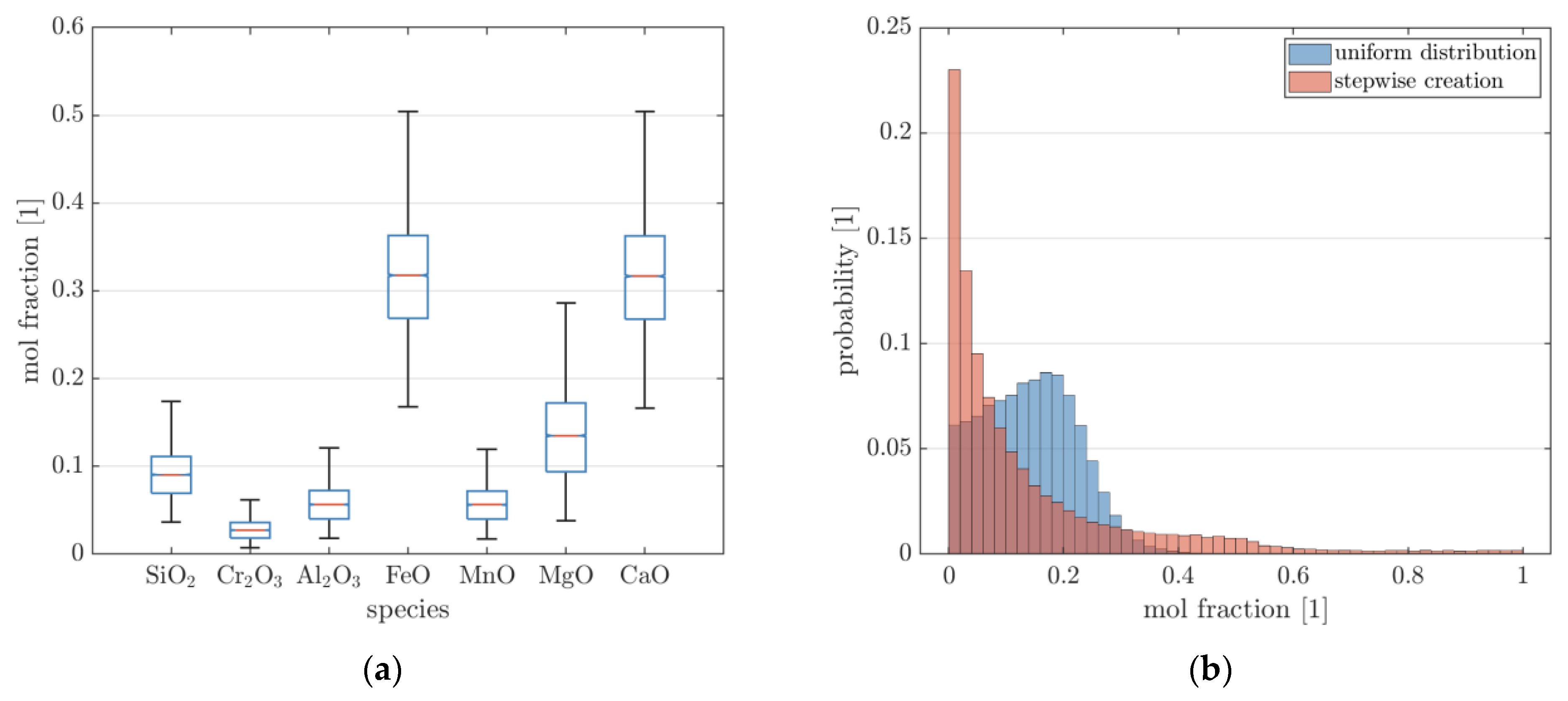
Figure 1a, the generated slag composition of the tapping scenario is shown in the form of a box plot. The slag consists mainly of FeO, CaO, and MgO with lower percentages of the remaining species. Figure 1b also shows the probability distribution of the molar fractions for the second scenario. As can be seen, when drawing from a uniform distribution with subsequent normalization, almost no samples exceed a mole fraction of 0.4. In contrast, when stepwise-creating the composition array, mole fractions of up to 1 can be reached. By nature, this results in a higher overall number of small mole fractions. The composition matrices from scenario 1 and 2 (with stepwise creation) are used in conjunction when training the model to prevent overfitting of the neural network to a specific situation.
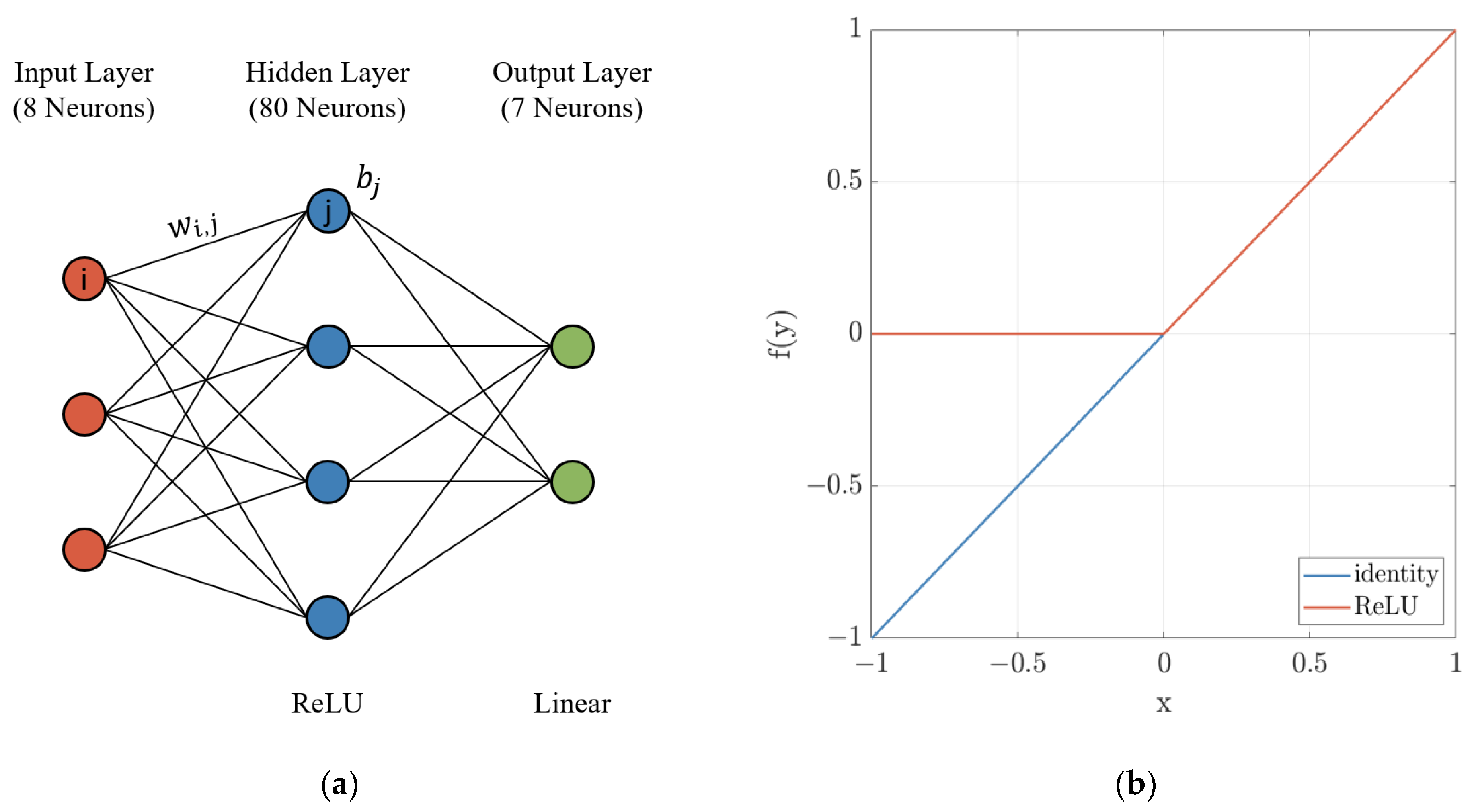
For approximation of the chemical activity, a shallow feedforward neural network was chosen. When applying neural nets, most computational effort is during training of the model weights. Predicting the output using the trained model is as simple as matrix multiplication and summation, as such computation of the prediction is not reliant on third-party libraries and can be implemented very efficiently. The network is composed of an input and output layer, as well as a single hidden layer with 80 neurons. The layout of the neural network is depicted in Figure 2a.
As shown in Equation (3), at each node, the input from the previous layer denoted by vj is first multiplied by a set of weights wij specific to the neuron i. Afterwards, the corresponding vector is cumulated, and a bias bi is added. The result x is passed onto the next layer by application of an activation function f(x). The output layer utilizes a linear activation function (identity) with a constant value as given by Equation (4), while the neurons within the hidden layer uses a rectified linear unit (ReLU) as stated in Equation (5). Both functions are visualized in Figure 2b. In the recent past, the ReLU has become the default choice for most feedforward networks [27]. While the advantages of the ReLU in terms of the learning rate are neglectable for small networks, it has been chosen in order to introduce a nonlinear transformation to the model. Stacking linear layers, the output would otherwise still be equivalent to a linear combination of the input arguments [28]. The model input consists of the temperature and composition of the slag. In theory, the chemical activity is also dependent on pressure. However, the melt–slag interface is located above the melt, with the pressure inside the EAF being reasonably close to atmospheric pressure. For this reason, the pressure dependency of the activity can be neglected. The output contains the activities of each species at the given temperature and composition.
x = j = 1 n w i j v j + b i
f l i n e a r x = a x
f R e L U x = x + x 2
Both the weights and biases of each neuron can be seen as parameters of the neural network. Starting from their initial values, during training, the parameters are adjusted such that the output of the network best matches the reference values. To achieve this, a backpropagation algorithm is applied. Starting from the output layer, the effect of each individual weight on the result is calculated by partial derivation of the obtained overall error. The weights can then be adjusted accordingly before the next iteration [
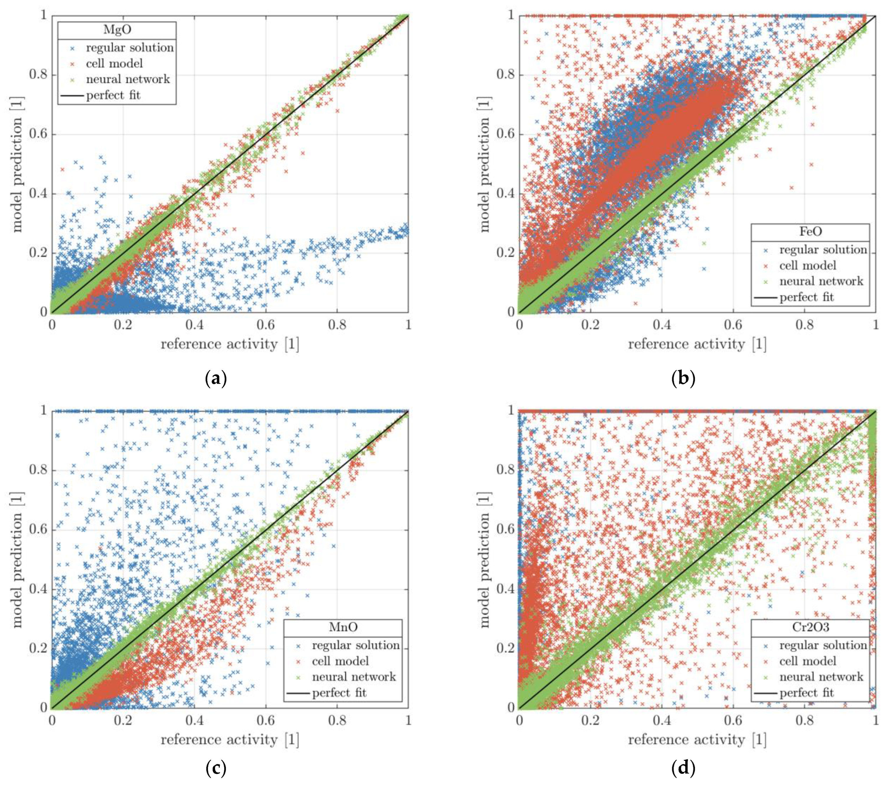
29]. This process is repeated until the output is within a specified tolerance or the maximum number of iterations is reached. In the upcoming section, the results of the surrogate model are compared to the previously used models. In this regard, the results are evaluated based on several metrics. A major aspect is the accuracy of the model prediction. As such, the deviation between the chemical activity calculated by each model and the reference values obtained with FactSage is assessed using the mean absolute error (MAE) as stated in Equation (6). Additionally, the adjusted coefficient of determination ( R 2 ) given in Equation (7) is calculated from the ratio of the residual (RSS) and total sum of squares (TSS). The coefficient is a popular measure for the quality of a fit and is often presented as the percentage of variance of the result which is explained by the linear relationship with the explanatory variables [30]. Finally, the 95% percentile is provided, representing the threshold within which 95% of the results fall. Likewise, 5% of the results have a deviation greater than the threshold. This metric can be interpreted as a worst-case analysis. Due to the dynamic nature of the EAF process, small deviations from the actual result can cancel each other out, while large deviations will significantly affect the overall result of the simulation.
M A E = 1 n f i y i
R 2 = 1 R S S T S S = 1 f i y i 2 y i y ¯ 2
On the other hand, the computation speed of the models is relevant, as the purpose of the surrogate model is not only to closely reproduce the reference value, but to do so in significantly less time than the previous models. In order to eliminate random fluctuations, the execution time is averaged for all samples within the validation set. The calculations are performed in serial, as this resembles the later usage in the EAF model. Furthermore, the computation time of the surrogate model is multiplied by a factor of 8 / 7 as it is missing the activity of phosphorus oxide. However, it can be argued that the complexity of the neural network remains largely unchanged, as the additional output only affects the size of matrices used for calculation but not the overall structure of the model.

3. Results

In Figure 3, the results of the surrogate model are displayed for MgO, FeO, MnO, and Cr2O3. In addition, the activities calculated using the previous models are shown. The solid line represents a perfect fit between the model results and the reference values obtained with FactSage. Values that exceed an activity of 1 are displayed at the corresponding boundary. The performance of the investigated models is also summarized in Table 2 using the previously outlined metrics. As can be seen from both Figure 3 and Table 2, the trained neural network is able to estimate the slag activity more reliably than the RS, as well as the cell model. With the only exception of Cr2O3 at activities close to 1, the surrogate model reproduces the FactSage results over the entire range of compositions. This corresponds to an average deviation of 0.016 at maximum and a 95% quantile threshold of 0.065. The coefficient of determination (R2) ranges from 0.97 to 0.99, showing an exceptional quality of the fit. In contrast, large deviations can be observed for the previous models. This is especially the case for the RS model. The poor representation can be partly attributed to the missing interaction parameters for Cr3+ with Fe2+, Mn2+, and P5+. This is confirmed by the substantial deviation for both the mean deviation and 95% percentile of Cr2O3. Nonetheless, the results of the RS also show deviations for the remaining species.
The RS model performs best for Al2O3 and SiO2, with R2 scores of 0.95 and 0.71, respectively. Overall, the cell model performs better than the RS model with an R2 of up to 0.97 for both MgO and CaO. However, the cell model also faces difficulties in determining the activity of FeO and Cr2O3. For both species, the activity deviates from the reference by 0.15 on average. In addition, the computational demand of the cell model is roughly 300 times larger when compared to that of the RS model. When running the EAF process model for a heat of 60 min, the ODE solver takes approximately 35,000 calculation steps depending on the smoothness of the furnace operation. By applying the cell model without further simplification, this results in an additional simulation time of over 340 s on the system used for the testing of the model.
In contrast, the neural network takes only about 0.1 s for 1000 iterations (4 s for the entire heat) and is, thus, on a similar scale as the RS model while providing significantly improved results. This comparison neglects the influence of the calculated slag activity on the simulation. In theory, an improved calculation of chemical activities could lead to a more continuous progression of chemical reactions within the model, further reducing the number of evaluation steps required by the solver. However, this is highly dependent on the general operation of the furnace and could not be reliably observed for the process model under investigation. Furthermore, within the process model, additional simplification and optimization is performed, reducing the overall numerical effort.

4. Discussion

Within this work, a shallow feedforward network is applied in order to approximate the chemical activity of the species within a metallurgical slag. The network is used as a surrogate within a comprehensive dynamic process model of the EAF in order to reduce the overall computational demand while maintaining a reasonable accuracy. For the training of the model, a large number of chemical compositions was created to reflect the different stages of the EAF process. The reference activities were then calculated using the commercial software FactSage. Afterwards, the dataset was split into separate datasets for the training and validation of the model. The accuracy of the neural network was compared to the results of the previously applied regular solution and cell model. During validation, it became evident that the neural network outperforms the previous models in terms of the prediction accuracy. At the same time, the computational complexity remained close to that of the regular solution model. This way, by implementing the surrogate model, the runtime of the process model can be minimized when performing, for example, optimization tasks. However, since the modelling approach is not based on physical principles, the neural network should not be used outside the range of the training data. Otherwise, the results may produce unexpectedly large deviations from the actual chemical activities. In such cases, it is advisable to retrain the model or integrate the original FactSage model. While it is possible to directly integrate FactSage’s calculation into the EAF process model, this is also associated with an increased overhead and a higher overall runtime.
Within the context of this work, FactSage was used both for the creation of the data used for the training of the surrogate model, as well as for reference when evaluating the results of the investigated models. Therefore, the applied neural network may not necessarily be better suited for calculating the chemical activities. The evaluation of the results only confirms that the model is able to better match the results provided by FactSage. Furthermore, Version 6.4 of the FTstel and FToxid databases are missing data on phosphorus oxide. As noted before, the phosphorus content of the steel is, however, a major concern for ensuring the targeted properties of the produced steel. In summary, the surrogate model is highly dependent on the availability of the underlying reference model and its ability to produce the desired output. That being said, the presented approach can be applied in various contexts and is not limited to the calculation of chemical activities. The benefit of employing a surrogate model in terms of computational effort is, however, dependent on the complexity of the original problem as well as the implementation of the applied methods.
On a side note, the considered EAF process model was implemented using the Python programming language for the reason of its open-source nature and accessibility. As an interpreter language, Python is, however, inherently slower than compiler languages such as C or Fortran [31,32]. Utilizing third-party libraries such as numba, the Python function can be compiled ahead of time [33]. The output of the trained neural network is calculated using basic operations such as matrix multiplication and summation. Therefore, it is not reliant on third-party libraries and can be easily implemented to work in conjunction with numba. This way, the calculation of the slag activity and, by extension, the entire EAF model can by pre-compiled, resulting in a further decrease in runtime.

Author Contributions

Conceptualization, A.R., L.S. and T.-N.E.; methodology, A.R., T.-N.E. and L.S.; software, A.R., T.-N.E. and L.S.; validation, A.R.; resources, T.E.; data curation, A.R. and L.S.; writing—original draft preparation, A.R.; writing—review and editing, A.R., L.S. and T.E.; visualization, A.R.; supervision, T.E.; project administration, T.E.; funding acquisition, T.E. All authors have read and agreed to the published version of the manuscript.

Funding

This research received no external funding.

Data Availability Statement

The original contributions presented in the study are included in the article, further inquiries can be directed to the corresponding author.

Conflicts of Interest

The authors declare no conflicts of interest.

References

  1. World Steel Association. World Steel in Figures: Concise Version; World Steel Association: Brussels, Belgium, 2023; Available online: https://worldsteel.org (accessed on 6 February 2024).
  2. Demus, T.; Reichel, T.; Schulten, M.; Echterhof, T.; Pfeifer, H. Increasing the sustainability of steel production in the electric arc furnace by substituting fossil coal with biochar agglomerates. Ironmak. Steelmak. 2016, 43, 564–570. [Google Scholar] [CrossRef]
  3. Kirschen, M.; Hay, T.; Echterhof, T. Process Improvements for Direct Reduced Iron Melting in the Electric Arc Furnace with Emphasis on Slag Operation. Processes 2021, 9, 402. [Google Scholar] [CrossRef]
  4. Hay, T.; Visuri, V.-V.; Aula, M.; Echterhof, T. A Review of Mathematical Process Models for the Electric Arc Furnace Process. Steel Res. Int. 2021, 92, 2000395. [Google Scholar] [CrossRef]
  5. Carlsson, L.S.; Samuelsson, P.B.; Jönsson, P.G. Predicting the Electrical Energy Consumption of Electric Arc Furnaces Using Statistical Modeling. Metals 2019, 9, 959. [Google Scholar] [CrossRef]
  6. Meier, T. Modellierung und Simulation des Elektrolichtbogenofens; Verlagshaus Mainz: Mainz, Germany, 2016; ISBN 978-3-95886-129-9. [Google Scholar]
  7. Logar, V.; Dovžan, D.; Škrjanc, I. Modeling and Validation of an Electric Arc Furnace: Part 1, Heat and Mass Transfer. ISIJ Int. 2012, 52, 402–412. [Google Scholar] [CrossRef]
  8. Logar, V.; Dovžan, D.; Škrjanc, I. Modeling and Validation of an Electric Arc Furnace: Part 2, Thermo-chemistry. ISIJ Int. 2012, 52, 413–423. [Google Scholar] [CrossRef]
  9. Pfeifer, H.; Nacke, B.; Beneke, F. Praxishandbuch Thermoprozesstechnik: Band II: Anlagen-Komponenten-Sicherheit, 3rd ed.; Vulkan: Essen, Germany, 2022; ISBN 9783802731228. [Google Scholar]
  10. Ben Bowman, K.K. Arc Furnace Physics, 1st ed.; Stahleisen: Düsseldorf, Germany, 2009; ISBN 978-3514007680. [Google Scholar]
  11. Graham, K.J. Integrated Ladle Metallurgy Control. Ph.D. Thesis, McMaster University, Hamilton, ON, Canada, 2008. [Google Scholar]
  12. MacRosty, R.D.M.; Swartz, C.L.E. Dynamic Modeling of an Industrial Electric Arc Furnace. Ind. Eng. Chem. Res. 2005, 44, 8067–8083. [Google Scholar] [CrossRef]
  13. Hay, T.; Reimann, A.; Echterhof, T. Improving the Modeling of Slag and Steel Bath Chemistry in an Electric Arc Furnace Process Model. Metall. Mater. Trans. B 2019, 50, 2377–2388. [Google Scholar] [CrossRef]
  14. Shampine, L.F.; Reichelt, M.W. The MATLAB ODE Suite. SIAM J. Sci. Comput. 1997, 18, 1–22. [Google Scholar] [CrossRef]
  15. Lupis, C.; Elliott, J. Generalized interaction coefficients: Part II: Free energy terms and the quasi-chemical theory. Acta Metall. 1966, 14, 1019–1032. [Google Scholar] [CrossRef]
  16. Pelton, A.D.; Bale, C.W. A modified interaction parameter formalism for non-dilute solutions. Metall. Trans. A 1986, 17, 1211–1215. [Google Scholar] [CrossRef]
  17. Basu, S.; Seetharaman, S.; Lahiri, A.K. Thermodynamics of Phosphorus and Sulphur Removal during Basic Oxygen Steelmaking. Steel Res. Int. 2010, 81, 932–939. [Google Scholar] [CrossRef]
  18. Michalek, K.; Čamek, L.; Gryc, K.; Tkadlečková, M.; Huczala, T.; Troszok, V. Desulphurization of the high-alloy and middle-alloy steels under the conditions of an eaf by means of synthetic slag based on CaO-Al2O3. Mater. Technol. 2012, 46, 297–303. [Google Scholar]
  19. Schrama, F.N.H.; Beunder, E.M.; van den Berg, B.; Yang, Y.; Boom, R. Sulphur removal in ironmaking and oxygen steelmaking. Ironmak. Steelmak. 2017, 44, 333–343. [Google Scholar] [CrossRef]
  20. Kirschen, M. Visualization of Slag Data for Efficient Monitoring and Improvement of Steelmaking Slag Operation in Electric Arc Furnaces, with a Focus on MgO Saturation. Metals 2021, 11, 17. [Google Scholar] [CrossRef]
  21. Ban-Ya, S. Mathematical Expression of Slag-Metal Reactions in Steelmaking Process by Quadratic Formalism Based on the Regular Solution Model. ISIJ Int. 1993, 33, 2–11. [Google Scholar] [CrossRef]
  22. Gaye, H.; Lehmann, J.; Matsumiya, T.; Yamada, W. A statistical thermodynamics model of slags: Applications to systems containing S, F, P2O5 and Cr oxides. In Proceedings of the 4th International Conference on Molten Slags and Fluxes, Sendai, Japan, 8–11 June 1992; ISIJ: Sendai, Japan, 1992; pp. 103–108. [Google Scholar]
  23. Hay, T. Mathematische Modellierung des Elektrostahlverfahrens. Ph.D. Thesis, RWTH Aachen University, Aachen, Germany, 2021. [Google Scholar]
  24. Xiao, Y.; Holappa, L. Thermodynamics of slags containing chromium oxides. In Proceedings of the INFACON 7, Trondheim, Norway, 11–14 June 1995; Norwegian Ferroalloy Research Organization (FFF): Trondheim, Norway, 1995. [Google Scholar]
  25. Bale, C.W.; Bélisle, E.; Chartrand, P.; Decterov, S.A.; Eriksson, G.; Gheribi, A.E.; Hack, K.; Jung, I.-H.; Kang, Y.-B.; Melançon, J.; et al. FactSage thermochemical software and databases, 2010–2016. Calphad 2016, 54, 35–53. [Google Scholar] [CrossRef]
  26. GTT, C. FactSage Database Overview. Available online: https://www.factsage.com/facthelp/FSNew_Databases.htm (accessed on 31 January 2024).
  27. Goodfellow, I.; Bengio, Y.; Courville, A. Deep Learning; MIT Press: Cambridge, MA, USA, 2016. [Google Scholar]
  28. Szandała, T. Review and Comparison of Commonly Used Activation Functions for Deep Neural Networks. In Bio-Inspired Neurocomputing; Bhoi, A., Mallick, P., Liu, C.M., Balas, V., Eds.; Springer: Singapore, 2021; pp. 203–224. ISBN 978-981-15-5495-7. [Google Scholar]
  29. Rumelhart, D.E.; Hinton, G.E.; Williams, R.J. Learning representations by back-propagating errors. Nature 1986, 323, 533–536. [Google Scholar] [CrossRef]
  30. Renaud, O.; Victoria-Feser, M.-P. A robust coefficient of determination for regression. J. Stat. Plan. Inference 2010, 140, 1852–1862. [Google Scholar] [CrossRef]
  31. Romer, T.H.; Lee, D.; Voelker, G.M.; Wolman, A.; Wong, W.A.; Baer, J.-L.; Bershad, B.N.; Levy, H.M. The structure and performance of interpreters. In Proceedings of the Seventh International Conference on Architectural Support for Programming Languages and Operating Systems, Cambridge, MA, USA, 1–4 October 1996; Association for Computing Machinery: New York, NY, USA, 1996; pp. 150–159, ISBN 0897917677. [Google Scholar]
  32. Barany, G. Python Interpreter Performance Deconstructed. In Proceedings of the Workshop on Dynamic Languages and Applications, Edinburgh, UK, 12 June 2014; Association for Computing Machinery: New York, NY, USA, 2014; pp. 1–9, ISBN 9781450329163. [Google Scholar]
  33. Anaconda. Numba: User Manual. Available online: https://numba.readthedocs.io/en/stable/user/index.html (accessed on 3 June 2024).
Figure 1. (a) Boxplot of generated mole fractions from slag composition at tapping; and (b) probability distribution for uniformly drawn and stepwise creation of composition.
Metals 14 00736 g001
Figure 2. (a) Structure of the neural network; and (b) response of the activation functions.
Metals 14 00736 g002
Figure 3. Activities obtained by the cell model and Gaussian process regression compared to the results from FactSage for relevant oxides in the slag: (a) magnesium oxide, (b) iron oxide, (c) manganese oxide, and (d) chromium oxide.
Metals 14 00736 g003
Table 1. Exemplary composition and temperature with upper and lower bounds.
TemperatureFeOCr2O3Al2O3MnOP2O5SiO2MgOCaO
UnitKwt.%
Slag * 35.62.56.16.40.311.99.625.8
Scenario 1: tappingLL17002012.52.505520
UL200050510100152550
Scenario 2: processLL170000000000
UL20001001001001000100100100
* analyzed slag contained further species such as S, TiO2, and V2O5.
Table 2. Overview of the performance of the applied models.
ModelExecution Time for 1000 SamplesSpeciesMAER295% Percentile
RS0.037 sSiO20.02790.710.1483
Cr2O30.8059−10.10.9995
Al2O30.00890.950.0563
FeO0.1523−0.090.3543
MnO0.0651−0.110.2815
MgO0.0846−0.050.2424
CaO0.0380−0.090.1097
Cell9.848 sSiO20.02890.650.1558
Cr2O30.14830.150.5462
Al2O30.01420.530.0480
FeO0.1582−0.180.3823
MnO0.03760.810.1210
MgO0.01450.970.0425
CaO0.00580.970.0191
ANN0.115 sSiO20.00860.970.0379
Cr2O30.01630.980.0655
Al2O30.00460.990.0201
FeO0.01120.990.0354
MnO0.00710.990.0232
MgO0.00680.990.0222
CaO0.00410.990.0137
Disclaimer/Publisher’s Note: The statements, opinions and data contained in all publications are solely those of the individual author(s) and contributor(s) and not of MDPI and/or the editor(s). MDPI and/or the editor(s) disclaim responsibility for any injury to people or property resulting from any ideas, methods, instructions or products referred to in the content.

