Multi Response Modelling and Optimisation of Copper Content and Heat Treatment Parameters of ADI Alloys by Combined Regression Grey-Fuzzy Approach

Abstract

This paper deals with the austempering of ductile iron (ADI) and clarifies the influential austempering parameters during the production of ADI. During the austempering process, the heat treatment parameters can be varied, thus influencing the final microstructure and, of course, the mechanical properties of ADI. To appropriately conduct experiments and obtain good results, an experimental plan was developed using the Design Expert 13 software. Along with the heat treatment parameters, the influence of the copper content on the ADI toughness, tensile strength, and elongation was determined. The obtained results from this experiment were used to develop unique mathematical models which describe the influences of heat treatment and copper content on the observed mechanical properties of ADI samples. These mathematical models can be applied to predict the analysed mechanical properties of ADI in the dependence of heat treatment parameters and copper content in base ductile iron. For the multi response optimisation of toughness, tensile strength, and elongation, a hybrid grey-fuzzy technique was presented as a significant contribution to the enhancement of the analysed mechanical properties. Consequently, the copper content and heat treatment parameter levels that resulted in the maximal mechanical properties’ functions were defined.

1. Introduction

Ductile iron is a solid, durable, and economically viable metal material whose production is increasing every year to meet the high demand on the market. Nodular cast iron has been intensively researched, with the main focus on improving its mechanical properties. This can be achieved by suitable heat treatment or by alloying with various alloying elements [1,2]. Ductile iron has good physical, mechanical, and technological properties that lead to rapid production growth such as surface-hardening ability, corrosion resistance, favourable strength, a high modulus of elasticity, and good castability, etc. Austempered ductile iron (ADI) is produced when ductile iron undergoes austempering heat treatment (H.T.) [3,4,5,6,7]. ADI is special because of its ausferrite microstructure, a mixture of carbon-enriched retained austenite and needle ferrite [8,9,10,11]. An ausferrite microstructure has properties superior to many iron and aluminium alloys. The austempered matrix has a better ductility and tensile strength ratio than any other types of ductile iron. Depending on the content of the alloying elements and heat treatment parameters, different mechanical properties of ADI can be achieved [12,13,14]. To properly austemper ductile iron, it must be austenitised at the proper temperature for certain amount of time, quenched at the austempering temperature, preferably in a salt bath, and air cooled to room temperature [15].

2. Materials and Experiment

Combining data from the available literature and data from previous research, the austempering H.T. parameters were determined. Also, the copper content range was established. Using these input parameters, a research methodology for investigation was developed. Since the research should be as close as possible to the actual heat treatment of ductile iron in order to obtain ADI, right ductile iron alloys were selected. Also, it was important to determine the proper shape and number of samples.

When it comes to the quenching medium, it was found that a salt bath is the best medium for austempering [16]. Other quenching mediums like lead or oil baths can be used, but they have worse properties when compared to salt baths. From previous research, it was determined that all heat treatment parameters have influence on the final microstructure and mechanical properties of ADI [16,17,18]. Of all the parameters, the austenitisation time has smallest influence on the final ADI properties, so this was not changed in this research.

It was found that the individual alloying elements have varying influences on the final ADI properties. Some, like copper, have a direct influence on strength and hardness increases, while others primarily influence ductility and toughness. Copper can easily be varied in ductile iron, since it is added to the ductile iron base melt as a pure element. Other alloying elements that are usually added are added as ferroalloys and so change the base melt chemical composition.

2.1. Experimental Plan

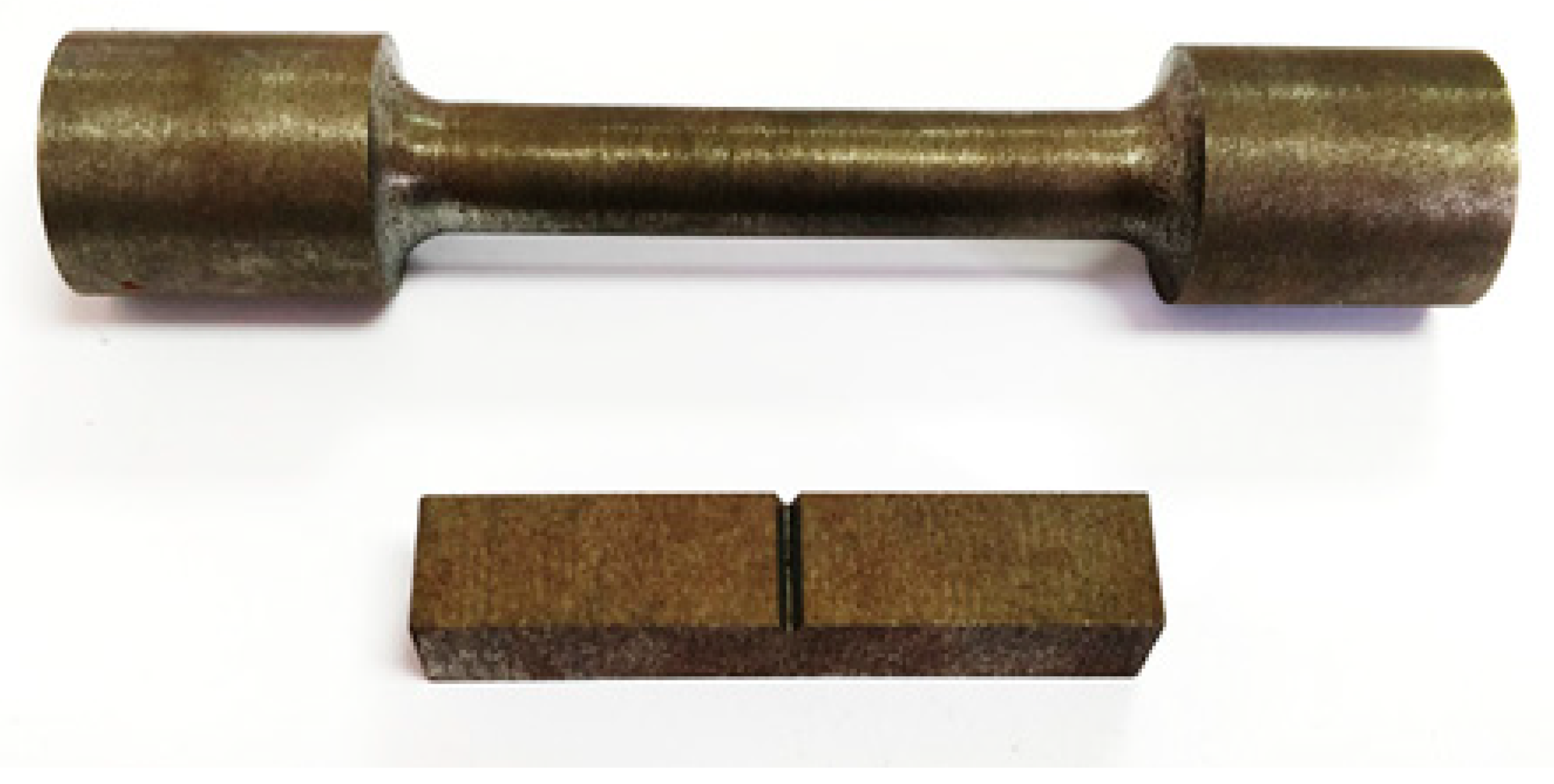
The development of an experimental plan for this study was conducted with the State-Ease Design Expert program. The first step was to define the categories and boundaries of the input parameters. This investigation consisted of three numerical input parameters with strict limits: an austenitizing temperature (T_A) from 850 °C to 950 °C, an austempering temperature (T_IZ) from 250 °C to 420 °C, and an austempering time (t_IZ) from 30 min to 120 min. The fourth and final input parameter was the copper content in the ductile iron. This is a categorical input parameter, as the copper content in each alloy was precisely defined and did not change during the investigation.

The ductile iron alloy copper contents used were 0.031; 0.32; 0.51; and 0.91 wt.% Cu. A D-optimal experimental design was used for these input parameters. Such an experiment design is mostly used in response surface methodology (RSM) when there are categorical and numerical input parameters at the same time. The D-optimal experimental design is an “alphabetically” optimal design developed to select the experimental points such that the variance associated with the estimates of certain model coefficients is minimised [19]. For the input constraints, the software determines the final experimental design, as shown in

Table 1. Plan of experiments.

Sample ID	Austenitisation Temperature, TA [°C]	Austempering Temperature, TIZ [°C]	Austempering Time, tIZ [°C]	Copper Content, [wt.% Cu]
503	897	383	101	0.031
504	947	345	87	0.031
505	904	282	48	0.031
507	850	250	86	0.031
508	850	384	42	0.031
509	850	420	120	0.031
510	887	420	30	0.031
511	950	352	30	0.031
512	950	420	120	0.031
514	910	250	120	0.031
516	950	420	60	0.031
517	850	250	30	0.031
518	948	258	31	0.031
519	850	309	120	0.031
520	950	250	93	0.031
602	850	390	120	0.32
603	850	420	78	0.32
605	950	250	30	0.32
607	922	315	120	0.32
608	899	293	30	0.32
609	950	349	68	0.32
610	850	335	30	0.32
612	950	420	120	0.32
613	950	250	120	0.32
614	850	250	49	0.32
615	950	420	120	0.32
619	865	250	120	0.32
620	944	420	30	0.32
626	922	250	86	0.32
629	885	399	43	0.32
701	950	420	30	0.51
703	950	420	120	0.51
704	917	420	72	0.51
705	866	250	30	0.51
706	850	331	68	0.51
707	950	312	86	0.51
708	950	420	120	0.51
709	850	420	120	0.51
710	950	250	30	0.51
711	917	420	72	0.51
712	896	335	98	0.51
715	850	250	120	0.51
716	917	344	30	0.51
717	900	250	120	0.51
718	850	420	30	0.51
801	950	420	120	0.91
802	900	339	120	0.91
803	950	381	30	0.91
814	879	271	76	0.91
821	904	420	71	0.91
807	850	291	30	0.91
808	904	250	30	0.91
809	950	420	120	0.91
810	850	420	120	0.91
811	850	367	87	0.91
812	904	250	30	0.91
813	950	250	58	0.91
815	950	250	120	0.91
822	850	250	120	0.91
818	850	420	30	0.91

. The number of output parameters, i.e., the number of tested mechanical properties of the ADI, does not affect the final number of samples. As seen in Table 1, 60 samples for toughness, tensile strength, and elongation testing were required. In order to accommodate for statistical errors, 3 sets with 60 samples were made.

2.2. Samples

The ductile iron alloys used in this research were donated by the Croatian foundry RS Metali with its Rapid Virovitica foundry. Although the production details are regarded as trade secrets, the whole melting process performed by the company is according to the ISO and EN standards when it comes to producing ductile iron. The company has an 80-year-old tradition in metal casting. Sand mixing and preparation was conducted using a DISA SAM 10/100 mixer and moulds were made using different DISAMATIC machines. Among other casts, they complied with EN 1563 standard [19] needed to produce EN-GJS-400 (Alloy 1), EN-GJS-500 (Alloy 2), EN-GJS-600 (Alloy 3), and EN-GJS-700 (Alloy 4) ductile iron casts, as they have for the purpose of this research. The company has special laboratories for sand analysis with special equipment, chemical composition analysis with a LECO GDS 500A analyser, visual inspection, inspection and control of dimensions, microstructural analysis with an OLYMPUS microscope, and the testing of mechanical properties using a SHIMADZU AG-X tensile testing machine according to the EN ISO 6892 standard [20]. As shown in

Table 2. Alloys’ chemical composition.

Alloy	C [wt.%]	Si [wt.%]	Mn [wt.%]	Cu [wt.%]	S [wt.%]	P [wt.%]	Cr [wt.%]	V [wt.%]	Ni [wt.%]	Mo [wt.%]	Al [wt.%]	Ti [wt.%]	Sn [wt.%]	W [wt.%]	Mg [wt.%]
1	3.63	2.61	0.135	0.031	0.0035	0.022	0.005	0.004	0.085	0.003	0.017	0.013	0.033	0.017	0.041
2	3.63	2.61	0.135	0.32	0.0035	0.022	0.005	0.004	0.085	0.003	0.017	0.013	0.033	0.017	0.041
3	3.63	2.61	0.135	0.51	0.0035	0.022	0.005	0.004	0.085	0.003	0.017	0.013	0.033	0.017	0.041
4	3.63	2.61	0.135	0.91	0.0035	0.022	0.005	0.004	0.085	0.003	0.017	0.013	0.033	0.017	0.041

, four ductile iron alloys with different copper contents were produced.

Rectangular ingots with dimensions of 25 × 25 × 190 mm were made from each alloy listed in Table 2, as shown in Figure 1.

A Maho CNC Machining Centre was used to machine each ingot and produce Charpy samples with a V-notch for toughness testing and appropriate samples for tensile testing, as shown in Figure 2. Toughness was tested according to EN ISO 148 [21] and tensile strength and elongation according to EN ISO 6892 [20].

2.3. Heat Treatment

The ductile iron samples were austenitised in a DEMITERM EASY 9 furnace (ESTHERM, Sveta Nedjelja, Croatia) without a protective atmosphere. The power of the furnace was 3 kW with a maximum temperature of 1150 °C, which was measured by a K-type thermocouple (NiCr-Ni). The samples were austenitised according to the test plan at different temperatures ranging from 850 °C to 950 °C, whereby the holding time at the austenitising temperature was the same for all samples, namely, 60 min. Immediately after austenitisation, the samples were quenched directly in a salt bath to obtain the ADI. The austempering of the ductile iron was carried out in a JPA 6-600 furnace (ESTHERM, Sveta Nedjelja, Croatia) with a power of 3.1 kW and a maximum temperature of 600 °C. The temperature was measured with a type K thermocouple (NiCr-Ni). AS 140 salt was used for the salt bath. The samples were austempered between 250 °C and 420 °C, with times varying between 30 min and 120 min.

After heat treatment, all Charpy samples were thoroughly ground and finely polished. Firstly, all samples were treated with 80, 100, and 120 grit metal abrasive papers to remove the oxide layer. The next step was grinding on the Handimet Grinder with 240, 320, 400, and 600 grit water abrasives. The final step was polishing using aluminium oxide (Al₂O₃) in water suspension as an abrasive.

3. Results and Discussion

Toughness testing was performed on Charpy’s Zwick/Roell RKP 450 pendulum. The test was performed in accordance with EN ISO 148 [21]. The initial energy of the pendulum was 450 J. The stroke velocity of the piston was 5 m/s. Six measurements of width and height around the V-notch were performed on each sample and their mean values were calculated. Prior to testing, the device was calibrated for each sample in such a way that the mean values of the sample dimensions were entered into the computer program of the pendulum.

The tensile strength and elongation tests were performed on a Zwick/Roell Z600 tensile testing machine at room temperature. The test was carried out in accordance with EN ISO 6892 [20]. The preload was 5 MPa and the test speed was 0.0007 1/s. On each sample, nine measurements of the diameter of the test tube body were made and their mean values were calculated. Before the test itself, the device was calibrated for each individual test tube in such a way that the mean diameter values were entered into the computer program of the device. The mean results of all mechanical properties are shown in

Table 3. Obtained mean results.

Sample ID	Toughness KV [J]	Tensile Strength UTS [MPa]	Elongation EL [%]	Sample ID	Toughness KV [J]	Tensile Strength UTS [MPa]	Elongation EL [%]
503	10.2	1050	7.9	602	9.3	914	3.1
504	8.8	1125	6.4	603	3.8	776	1.1
505	6.2	1205	4.1	605	3.5	955	0.8
507	5.7	1000	3.6	607	7.1	1210	1.9
508	11.9	809	9.9	608	6.6	1270	1.7
509	4.0	834	2.3	609	8.5	942	2.8
510	7.5	980	5.2	610	10.7	825	3.8
511	8.1	1000	6.1	612	3.7	915	1.0
512	2.9	932	0.8	613	4.3	1230	1.2
514	3.6	1410	1.1	614	5.6	798	1.5
516	4.5	905	2.9	615	3.4	785	0.4
517	6.6	1070	4.4	619	4.1	1200	1.2
518	3.3	1120	0.9	620	8.6	747	2.9
519	6.6	1110	4.3	626	4.6	1240	1.3
520	3.7	1270	1.7	629	9.8	914	3.3
701	9.7	730	8.2	801	4.4	799	1.2
703	3.8	840	1.0	802	10.6	703	5.3
704	5.7	820	1.7	803	9.2	752	2.4
705	5.4	1240	1.3	807	7.8	1130	2.1
706	9.0	929	4.8	808	6.3	773	1.7
707	6.6	1230	2.7	809	7.2	1050	1.8
708	4.0	837	1.1	810	5.5	1310	1.6
709	3.8	855	1.0	811	2.7	806	0.8
710	3.2	1200	0.7	812	4.4	689	1.2
711	5.5	951	1.4	813	10.6	832	3.5
712	8.6	1260	4.7	814	4.0	1280	1.0
715	6.1	1180	2.2	815	5.2	1140	1.5
716	8.2	1080	3.8	818	2.9	1260	0.9
717	6.1	1300	2.0	821	5.1	963	1.4
718	9.9	697	10.0	822	9.7	715	2.9

.

3.1. Regression Models for Toughness, Tensile Strength, and Elongation

The obtained toughness, tensile strength, and elongation mean results were entered into the Design Expert program and statistically analysed. Based on a reverse elimination regression analysis of the measured mechanical properties, mathematical models were obtained. These models express the statistical relationship between the variables. The analysis starts with the full model, i.e., the inclusion of all possible variables. In the next step, parts of the model with the highest p-value are hierarchically removed. The elimination of model parts is stopped when the maximum p-value is less than or equal to the set limit. The limit is usually set at 5% (p-value ≦ 0.05) [22].

Analyses of variance for all measured responses are shown in

Table 4. Analyses of variance for all measured responses.

	Toughness KV [J]		Tensile Strength UTS [MPa]		Elongation EL [%]
	F Value	p-Value	F Value	p-Value	F Value	p-Value
MODEL	24.71	<0.0001	26.36	<0.0001	28.33	<0.0001
A − TA [°C]	44.87	<0.0001	37.43	<0.0001	47.37	<0.0001
B − TIZ [°C]	61.33	<0.0001	599.80	<0.0001	108.60	<0.0001
C − tIZ [min]	70.61	<0.0001	23.92	0.0002	70.64	<0.0001
D − wt.%Cu	2.35	0.0932	22.33	<0.0001	52.01	<0.0001
AB	1.95	0.1728	5.00	0.0399	/	/
AC	9.69	0.0041	3.81	0.0687	22.58	<0.0001
AD	/	/	0.4135	0.7456	6.38	0.0028
BC	66.84	<0.0001	0.5798	0.4575	48.01	<0.0001
BD	0.1248	0.9447	4.24	0.0220	11.76	<0.0001
CD	0.4711	0.7047	9.66	0.0007	16.40	<0.0001
A2	3.01	0.0933	51.62	<0.0001	0.1358	0.7160
B2	232.59	<0.0001	1.91	0.1861	144.14	<0.0001
C2	0.1188	0.7328	0.0004	0.9839	0.6096	0.4433
ABC	/	/	2.95	0.1054	/	/
ACD	/	/	3.12	0.0552	/	/
BCD	5.12	0.0058	2.15	0.1336	24.07	<0.0001
A2B	/	/	10.85	0.0046	/	/
A2C	/	/	14.92	0.0014	18.33	0.0003
A2D	/	/	10.13	0.0006	6.93	0.0019
AC2	/	/	3.48	0.0805	/	/
B2C	22.02	<0.0001	/	/	8.93	0.0068
B2D	2.79	0.0580	2.72	0.0789	11.97	<0.0001
BC2	20.20	0.0001	12.30	0.0029	7.39	0.0125
C2D	4.25	0.0131	4.19	0.0229	6.77	0.0021
A3	/	/	1.77	0.2026	5.26	0.0318
B3	58.64	<0.0001	/	/	42.92	<0.0001
C3	/	/	14.11	0.0017	/	/
Lack of Fit	0.9409	0.5948	0.3872	0.9118	3.33	0.0940
Std. Dev.	0.6900		45.02		0.5240
Mean	6.30		998.20		2.76
C.V. (%)	10.94		4.51		19.00
R2	0.9624		0.9861		0.9794
Adj − R2	0.9234		0.9487		0.9449
Pre − R2	0.8149		0.7822		0.7882
Adeq. Pre.	16.8906		19.4512		22.2665
PRESS	67.87		5.075 + 105		62.24
−2 Log Like.	82.12		547.82		32.52
BIC	209.04		727.97		188.10
AICc	214.98		899.82		249.66

. In Table 4, Std. Dev., Mean, C.V., R², and other statistical information are also shown.

As shown in Table 4, all used models are significant. For the measured Toughness KV [J], the model F-value is 24.7, for the measured UTS [MPa], the model F-value is 26.36, and for the measured EL [%], the model F-value is 28.33. There is only a 0.01% chance that F-values this large could occur due to noise. All p-values less than 0.0500 indicate that the model terms are significant and values greater than 0.1000 indicate that the model terms are not significant. Fit statistics for the Toughness KV [J] show that the Predicted R² of 0.8149 is in reasonable agreement with the Adjusted R² of 0.9234, i.e., the difference is less than 0.2. Adeq. Precision measures the signal to noise ratio. A ratio greater than four is desirable. The obtained ratio of 16.8906 indicates an adequate signal, which means the model can be used to navigate the design space. Similarly, for UTS [MPa], the Predicted R² of 0.7822 is in reasonable agreement with the Adjusted R² of 0.9487, i.e., the difference is also less than 0.2. The Adeq Precision ratio of 19.4512 indicates an adequate signal stating that the model can be used for design space navigation. Finaly, for the change in EL [%], the Predicted R² of 0.7882 is in reasonable agreement with the Adjusted R² of 0.9449, with a difference of less than 0.2. The Adeq Precision ratio of 22.2665 indicates an adequate signal.

The models (1)–(3) indicate a significant influence of the austenitising temperature, the austempering temperature, and the austempering time on the mechanical properties for 0.031 wt.% Cu, as well as the interaction of these three parameters.

$$\begin{array}{c}KV=145.67595+0.25510·T_A-2.40286·T_{IZ}-0.18896·t_{IZ}+4.43388·{10}^{-5}·T_A·t_{IZ}\\ +1.88032·{10}^{-4}·T_A·t_{IZ}+1.63899·{10}^{-3}·T_{IZ}·t_{IZ}-1.66566·{10}^{-4}·{T_A}^2+7.59884·{10}^{-3}·{T_{IZ}}^2\\ -2.95758·{10}^{-3}·{t_{IZ}}^2-4.40148{·10}^{-6}·{T_{IZ}}^2·t_{IZ}+8.09914{·10}^{-6}·T_{IZ}·{t_{IZ}}^2-7.79917{·10}^{-6}·{T_{IZ}}^3\end{array}$$

(1)

$$\begin{array}{c}UTS=-6.08992·{10}^5+1839.01556·T_A+292.89941·T_{IZ}+467.10166·t_{IZ}\\ -0.65579·T_A·T_{IZ}-1.25956·T_A·t_{IZ}+0.14796·T_{IZ}·tiz-1.81736·{T_A}^2\\ -4.42801{·10}^{-3}·{T_{IZ}}^2+0.96970·{t_{IZ}}^2-1.00378{·10}^{-4}·T_A·T_{IZ}·t_{IZ}\\ +3.66155{·10}^{-4}·{T_A}^2·T_{IZ}+7.57270{·10}^{-4}·{T_A}^2·t_{IZ}\\ -3.98689{·10}^{-4}·T_A·{t_{IZ}}^2-4.52557{·10}^{-4}·T_{IZ}·{t_{IZ}}^2\\ +5.87858{·10}^{-4}·{T_A}^3-1.89040{·10}^{-3}·{t_{IZ}}^3\end{array}$$

(2)

$$\begin{array}{c}EL=-7667.34493+26.67159·T_A-1.50760·T_{IZ}-8.22222·t_{IZ}\\ +0.018194·T_A·t_{IZ}+9.29120{·10}^{-4}·T_{IZ}·t_{IZ}-0.030267·{T_A}^2\\ +5.06811{·10}^{-3}·{T_{IZ}}^2-1.95517{·10}^{-3}·{t_{IZ}}^2-9.99750{·10}^{-6}·{T_A}^2·t_{IZ}\\ -2.35910{·10}^{-6}·{T_{IZ}}^2·t_{IZ}+3.95258{·10}^{-6}·T_{IZ}·{t_{IZ}}^2\\ +1.14164{·10}^{-5}·{T_A}^3-5.40137{·10}^{-6}·{T_{IZ}}^3\end{array}$$

(3)

The models (4)–(6) show the influence of the input parameters on the mechanical properties for 0.32 wt.% Cu.

$$\begin{array}{c}KV=148.12099+0.25510·T_A-2.41076·T_{IZ}-0.25656·t_{IZ}+4.43388·{10}^{-5}·T_A·t_{IZ}\\ +1.88032·{10}^{-4}·T_A·t_{IZ}+1.43323·{10}^{-3}·T_{IZ}·t_{IZ}-1.66566·{10}^{-4}·{T_A}^2+7.63628·{10}^{-3}·{T_{IZ}}^2\\ -2.06508·{10}^{-3}·{t_{IZ}}^2-4.40148{·10}^{-6}·{T_{IZ}}^2·t_{IZ}+8.09914{·10}^{-6}·T_{IZ}·{t_{IZ}}^2-7.79917{·10}^{-6}·{T_{IZ}}^3\end{array}$$

(4)

$$\begin{array}{c}UTS=-6.39820·{10}^5+1906.58193·T_A+294.62510·T_{IZ}+473.17620·t_{IZ}\\ -0.65579·T_A·T_{IZ}-1.26495·T_A·t_{IZ}+0.15624·T_{IZ}·t_{IZ}-1.85485·{T_A}^2\\ -7.49854{·10}^{-3}·{T_{IZ}}^2+0.94833·{t_{IZ}}^2-1.00378{·10}^{-4}·T_A·T_{IZ}·t_{IZ}\\ +3.66155{·10}^{-4}·{T_A}^2·T_{IZ}+7.57270{·10}^{-4}·{T_A}^2·t_{IZ}\\ -3.98689{·10}^{-4}·T_A·{t_{IZ}}^2-4.52557{·10}^{-4}·T_{IZ}·{t_{IZ}}^2\\ +5.87858{·10}^{-4}·{T_A}^3-1.89040{·10}^{-3}·{t_{IZ}}^3\end{array}$$

(5)

$$\begin{array}{c}EL=-7592.28019+26.56738·T_A-1.73781·T_{IZ}-8.32882·t_{IZ}\\ +0.018194·T_A·t_{IZ}+8.66694{·10}^{-4}·T_{IZ}·t_{IZ}-0.030197·{T_A}^2\\ +5.40954{·10}^{-3}·{T_{IZ}}^2-1.03789{·10}^{-3}·{t_{IZ}}^2-9.99750{·10}^{-6}·{T_A}^2·t_{IZ}\\ -2.35910{·10}^{-6}·{T_{IZ}}^2·t_{IZ}+3.95258{·10}^{-6}·T_{IZ}·{t_{IZ}}^2\\ +1.14164{·10}^{-5}·{T_A}^3-5.40137{·10}^{-6}·{T_{IZ}}^3\end{array}$$

(6)

The models (7)–(9) represent how the tested mechanical results are influenced by the heat treatment parameters for 0.51 wt.% Cu.

$$\begin{array}{c}KV=165.13924+0.25510·T_A-2.54953·T_{IZ}-0.089985·t_{IZ}+4.43388·{10}^{-5}·T_A·t_{IZ}\\ +1.88032·{10}^{-4}·T_A·t_{IZ}+1.27135·{10}^{-3}·T_{IZ}·t_{IZ}-1.66566·{10}^{-4}·{T_A}^2+7.85964·{10}^{-3}·{T_{IZ}}^2\\ -2.74285·{10}^{-3}·{t_{IZ}}^2-4.40148{·10}^{-6}·{T_{IZ}}^2·t_{IZ}+8.09914{·10}^{-6}·T_{IZ}·{t_{IZ}}^2-7.79917{·10}^{-6}·{T_{IZ}}^3\end{array}$$

(7)

$$\begin{array}{c}UTS=-5.99065·{10}^5+1815.73686·T_A+294.17936·T_{IZ}+482.65118·t_{IZ}\\ -0.65579·T_A·T_{IZ}-1.27321·T_A·t_{IZ}+0.16046·T_{IZ}·t_{IZ}-1.80403·{T_A}^2\\ -8.40833{·10}^{-3}·{T_{IZ}}^2+0.92111·{t_{IZ}}^2-1.00378{·10}^{-4}·T_A·T_{IZ}·t_{IZ}\\ +3.66155{·10}^{-4}·{T_A}^2·T_{IZ}+7.57270{·10}^{-4}·{T_A}^2·t_{IZ}\\ -3.98689{·10}^{-4}·T_A·{t_{IZ}}^2-4.52557{·10}^{-4}·T_{IZ}·{t_{IZ}}^2\\ +5.87858{·10}^{-4}·{T_A}^3-1.89040{·10}^{-3}·{t_{IZ}}^3\end{array}$$

(8)

$$\begin{array}{c}EL=-7100.09447+25.42719·T_A-1.62367·T_{IZ}-8.22609·t_{IZ}\\ +0.018194·T_A·t_{IZ}+4.21370{·10}^{-4}·T_{IZ}·t_{IZ}-0.029568·{T_A}^2\\ +5.30794{·10}^{-3}·{T_{IZ}}^2-8.15450{·10}^{-3}·{t_{IZ}}^2-9.99750{·10}^{-6}·{T_A}^2·t_{IZ}\\ -2.35910{·10}^{-6}·{T_{IZ}}^2·t_{IZ}+3.95258{·10}^{-6}·T_{IZ}·{t_{IZ}}^2\\ +1.14164{·10}^{-5}·{T_A}^3-5.40137{·10}^{-6}·{T_{IZ}}^3\end{array}$$

(9)

Using models (10)–(12), it is possible to determine the influence of the starting parameters on the toughness, tensile strength, and elongation 0.91 wt.% Cu.

$$\begin{array}{c}KV=143.80631+0.25510·T_A-2.40759·T_{IZ}-0.10427·t_{IZ}+4.43388·{10}^{-5}·T_A·t_{IZ}\\ +1.88032·{10}^{-4}·T_A·t_{IZ}+1.47783·{10}^{-3}·T_{IZ}·t_{IZ}-1.66566·{10}^{-4}·{T_A}^2+7.62424·{10}^{-3}·{T_{IZ}}^2\\ -3.11701·{10}^{-3}·{t_{IZ}}^2-4.40148{·10}^{-6}·{T_{IZ}}^2·t_{IZ}+8.09914{·10}^{-6}·T_{IZ}·{t_{IZ}}^2-7.79917{·10}^{-6}·{T_{IZ}}^3\end{array}$$

(10)

$$\begin{array}{c}UTS=-5.55940·{10}^5+1726.60476·T_A+281.23021·T_{IZ}+454.97690·t_{IZ}\\ -0.65579·T_A·T_{IZ}-1.24121·T_A·t_{IZ}+0.16451·T_{IZ}·t_{IZ}-1.75582·{T_A}^2\\ +0.010317·{T_{IZ}}^2+0.89394·{t_{IZ}}^2-1.00378{·10}^{-4}·T_A·T_{IZ}·t_{IZ}\\ +3.66155{·10}^{-4}·{T_A}^2·T_{IZ}+7.57270{·10}^{-4}·{T_A}^2·t_{IZ}\\ -3.98689{·10}^{-4}·T_A·{t_{IZ}}^2-4.52557{·10}^{-4}·T_{IZ}·{t_{IZ}}^2\\ +5.87858{·10}^{-4}·{T_A}^3-1.89040{·10}^{-3}·{t_{IZ}}^3\end{array}$$

(11)

$$\begin{array}{c}EL=-7773.39035+26.99707·T_A-1.78732·T_{IZ}-8.31784·t_{IZ}\\ +0.018194·T_A·t_{IZ}+9.67449{·10}^{-4}·T_{IZ}·t_{IZ}-0.030440·{T_A}^2\\ +5.46521{·10}^{-3}·{T_{IZ}}^2-1.22236{·10}^{-3}·{t_{IZ}}^2-9.99750{·10}^{-6}·{T_A}^2·t_{IZ}\\ -2.35910{·10}^{-6}·{T_{IZ}}^2·t_{IZ}+3.95258{·10}^{-6}·T_{IZ}·{t_{IZ}}^2\\ +1.14164{·10}^{-5}·{T_A}^3-5.40137{·10}^{-6}·{T_{IZ}}^3\end{array}$$

(12)

Figure 3 shows the response surfaces for the toughness of the 0.031 wt.% Cu samples at different austenitising temperatures.

As shown in Figure 3, the toughness increases significantly with an increasing austempering temperature. This increase is evident up to about 370 °C. Above the austempering temperature of 370 °C, the toughness decreases. The toughness qualitatively monitors the change in the volume fraction of the retained austenite with the change in the austempering temperature [23]. The high values of toughness obtained on the austempered samples at temperatures around 370 °C can be explained by the optimum retained austenite content of the microstructure of the test samples. At temperatures above 370 °C, the volume fraction of the retained austenite decreases as the ausferrite decomposes into ferrite and carbides during the second stage of transformation. This undesirable transformation results in toughness degradation. Similar results were obtained for alloys of austempered ductile iron alloyed with copper, nickel, and molybdenum [24]. As shown in [25,26], the fracture impact energy can be qualitatively related to the dynamic and static toughness measured by Charpy using V-notch samples. Therefore, both the toughness and the fracture impact energy are expected to increase with an increasing volume of retained austenite.

For the 0.031 wt.% Cu alloy, austenitised at 850 °C and austempered at 378 °C for 30 min, a maximum toughness of 11.5 J is achieved. At an austenitising temperature of 900 °C, austempering temperature of 377 °C, and austempering time of 30 min, a maximum toughness of 10.9 J is achieved. The same alloy austenitised at 950 °C and austempered at 376 °C for 30 min, there is an obtained maximum toughness of 9.4 J.

Figure 4 shows the response surfaces for the toughness of the 0.32 wt.% Cu samples at different austenitising temperatures.

For the 0.32 wt.% Cu alloy, austenitised at 850 °C and austempered at 383 °C for 30 min, a maximum toughness of 12.9 J is achieved. At an austenitising temperature of 900 °C, austempering temperature of 382 °C, and austempering time of 30 min, a maximum toughness of 12.2 J is achieved. The same alloy austenitized at 950 °C and austempered at 382 °C for 30 min obtained a maximum toughness of 10.7 J.

Figure 5 shows the response surfaces for the toughness of the 0.51 wt.% Cu samples at different austenitising temperatures.

For the 0.51 wt.% Cu alloy, austenitised at 850 °C and austempered at 392 °C for 30 min, a maximum toughness of 12 J is achieved. At an austenitising temperature of 900 °C, austempering temperature of 392 °C, and austempering time of 30 min, a maximum toughness of 11.5 J is achieved. The same alloy austenitized at 950 °C and austempered at 392 °C for 30 min obtained a maximum toughness of 10 J.

Figure 6 shows the response surfaces for the toughness of the 0.91 wt.% Cu samples at different austenitising temperatures.

For the 0.91 wt.% Cu alloy, austenitised at 850 °C and austempered at 380 °C for 30 min, a maximum toughness of 12.2 J is achieved. At an austenitising temperature of 900 °C, austempering temperature of 380 °C, and austempering time of 30 min, a maximum toughness of 11.5 J is achieved. The same alloy austenitised at 950 °C and austempered at 380 °C for 30 min obtained a maximum toughness of 9.8 J.

It is clear from all the response surfaces shown that the toughness increases after heat treatment with an increase in the copper content. Also, with an increasing austenitisation temperature and austempering time, the toughness decreases, as does the volume fraction of the retained austenite.

Figure 7 shows the response surfaces for the tensile strength of the 0.031 wt.% Cu samples at different austenitising temperatures, while Figure 8 shows the response surfaces for the elongation of the same alloys.

According to Figure 7, the tensile strength increases significantly with the extension of the holding time at the austempering temperature, but decreases with an increase in the austempering temperature [27]. The change in the tensile strength qualitatively follows the change in hardness, and as the hardness increases, so does the strength. The reason for this is a change in the volume fraction of the residual austenite and lower carbon diffusion [23]. It can be seen from Figure 8 that the extensibility increases with an increase in the austempering temperature. This increase is evident up to about 370 °C. Above the austempering temperature of 370 °C, there is a drop in ductility. As well as impact fracture action, ductility qualitatively follows the change in volume fraction of the residual austenite with change in the austempering temperature. The high elongation values obtained for samples austempered at temperatures around 370 °C can be explained by the optimal volume fraction of the residual austenite in the microstructure of the test tubes. At temperatures above 370 °C, the volume fraction of the residual austenite decreases because the ausferrite decomposes into ferrite and carbides during the second stage of transformation. This undesirable transformation results in degradation of mechanical properties, both hardness and impact fracture action. Similar results were obtained for alloys of austempering ductile cast iron alloyed with copper, nickel, and molybdenum [24]. From the presented results of ductility and the volume fraction of residual austenite for all alloys, it is evident that, with an increase in the volume fraction of residual austenite, the ductility also increases.

For the 0.031 wt.% Cu alloy, austenitised at 850 °C and austempered at 250 °C for 120 min, a maximum tensile strength of 1180 MPa is achieved. For the same austenitisation temperature, amaximum elongation of 9.7% is achieved when austempered at 370 °C for 40 min. At an austenitising temperature of 900 °C, austempering temperature of 250 °C, and austempering time of 120 min, a maximum tensile strength of 1410 MPa is achieved. For the same austenitisation temperature, a maximum elongation of 8.6% is achieved when austempered at 370 °C for 80 min. The same alloy austenitised at 950 °C and austempered at 250 °C for 120 min obtained a maximum tensile strength of 1400 MPa. For the same austenitisation temperature, a maximum elongation of 7% is achieved when austempered at 360 °C for 55 min.

Figure 9 shows the response surfaces for the tensile strength of the 0.32 wt.% Cu samples at different austenitising temperatures, while Figure 10 shows the response surfaces for elongation of the same alloys.

For the 0.32 wt.% Cu alloy, austenitised at 850 °C and austempered at 250 °C for 120 min, a maximum tensile strength of 1060 MPa is achieved. For the same austenitisation temperature, a maximum elongation of 5.6% is achieved when austempered at 370 °C for 30 min. At an austenitizing temperature of 900 °C, austempering temperature of 250 °C, and austempering time of 115 min, a maximum tensile strength of 1370 MPa is achieved. For the same austenitisation temperature, a maximum elongation of 4.9% is achieved when austempered at 365 °C for 120 min. The same alloy austenitized at 950 °C and austempered at 250 °C for 120 min obtained a maximum tensile strength of 1230 MPa. For the same austenitisation temperature, a maximum elongation of 4.4% is achieved when austempered at 390 °C for 30 min.

Figure 11 shows the response surfaces forthe tensile strength of the 0.51 wt.% Cu samples at different austenitising temperatures, while Figure 12 shows the response surfaces for the elongation of the same alloys.

For the 0.51 wt.% Cu alloy, austenitised at 850 °C and austempered at 250 °C for 117 min, a maximum tensile strength of 1180 MPa is achieved. For the same austenitisation temperature, a maximum elongation of 5.6% is achieved when austempered at 385 °C for 30 min. At an austenitising temperature of 900 °C, austempering temperature of 250 °C, and austempering time of 30 min, a maximum tensile strength of 1390 MPa is achieved. For the same austenitisation temperature, a maximum elongation of 4.9% is achieved when austempered at 370 °C for 120 min. The same alloy austenitized at 950 °C and austempered at 250 °C for 105 min, there is an obtained maximum tensile strength of 1340 MPa. For the same austenitisation temperature, a maximum elongation of 4.4% is achieved when austempered at 385 °C for 30 min.

Figure 13 shows the response surfaces for the tensile strength of the 0.91 wt.% Cu samples at different austenitising temperatures, while Figure 14 shows the response surfaces for the elongation of the same alloys.

For the 0.91 wt.% Cu alloy, austenitised at 850 °C, austempered at 250 °C for 30 min, a maximum tensile strength of 1210 MPa is achieved. For the same austenitisation temperature, a maximum elongation of 4.4% is achieved when austempered at 385 °C for 30 min. At an austenitising temperature of 900 °C, austempering temperature of 250 °C, and austempering time of 30 min, a maximum tensile strength of 1310 MPa is achieved. For the same austenitisation temperature, a maximum elongation of 5.9% is achieved when austempered at 380 °C for 120 min. The same alloy austenitized at 950 °C and austempered at 250 °C for 105 min, there is an obtained maximum tensile strength of 1330 MPa. For the same austenitisation temperature, a maximum elongation of 3.7% is achieved when austempered at 380 °C for 120 min.

It can be seen that with an increase in copper content and a longer holding time at the austenitising temperature for a constant austenitising temperature, the tensile strength of the samples decreases after heat treatment. The change in tensile strength follows the trend of the change in hardness, while the elongation follows the trend in the change of the impact fracture action. Up to about 370 °C, the extensibility increases and, after that, it decreases with an increasing austempering temperature. With an increase in the austenitisation temperature and holding time at the austempering temperature, the ductility decreases, as does the volume fraction of residual austenite.

3.2. Multi Response Optimisation of Mechanical Properties by Grey-Fuzzy Approach

The aim of this chapter is to conduct the optimisation of all the analysed mechanical properties’ responses and to find out the parameter values that result in the maximal toughness, tensile strength, and elongation. This optimisation procedure will be performed by the application of a hybrid grey-fuzzy approach that combines grey relational analysis (GRA) and the fuzzy logic technique. The main advantage of chosen multi response optimisation approach is the absence of complex algorithms and mathematical modelling requirements. This hybrid grey-fuzzy optimization technique is relatively new in scientific applications. A few authors have already successfully applied this kind of methodology to optimise various processes [28,29,30,31,32].

The GRA method analyses numerical data sets of various responses to determine the level of correspondence between the ideal and real experimental (empirical) response values. The observed level of similarity between the ideal and real response values is expressed by grey relational coefficients (GRC). If the ideal and experimental response value are the same, then the GRC has a value of one. The GRA transforms multiple responses into a single response expressed by grey relational grade (GRG). The option with the highest GRG represents the optimal solution for all analysed responses. Consequently, from this result, the input parameter values that lead to the highest GRG value can be defined.

In order to conduct GRA, several steps must be fulfilled. The first step includes the normalisation of analysed responses. To decrease variability in the responses, raw data need to be normalised in the range [0, 1]. Depending on the objective function, maximum, minimum, or nominal different equations can be applied. In this case, the objective function for all responses, the mechanical properties of ADI alloys, is maximum, so normalisation was conducted following Equation (13).

$$X_i^{*}(k)=\frac{X_i^0\left(k\right)-min{ X}_i^0\left(k\right)}{max{ X}_i^0\left(k\right)-min{ X}_i^0\left(k\right)}$$

(13)

where: $X_i^0\left(k\right)$ is the original sequence, $X_i^{*}\left(k\right)$ is the sequence after data pre-processing, $min{ X}_i^0\left(k\right)$ is the smallest value in $X_i^0\left(k\right)$, and $max{ X}_i^0\left(k\right)$ is the largest value in $X_i^0\left(k\right)$.

The second step in the GRA process is calculation of the GRC. The GRC is calculated following Equation (14).

$${\xi }_i(k)=\frac{{\mathsf{\Delta }}_{min}+\xi {\mathsf{\Delta }}_{max}}{{\mathsf{\Delta }}_{0i}\left(k\right)+\xi {\mathsf{\Delta }}_{max}}$$

(14)

${\mathsf{\Delta }}_{0i}\left(k\right)$, ${\mathsf{\Delta }}_{min},$ and ${\mathsf{\Delta }}_{max}$ are calculated using Equations (15)–(17).

$${\mathsf{\Delta }}_{0i}\left(k\right)=‖X_0^{*}\left(k\right)-X_i^{*}\left(k\right)‖$$

(15)

$${\mathsf{\Delta }}_{max}=maxmax‖X_0^{*}\left(k\right)-X_i^{*}\left(k\right)‖$$

(16)

$${\mathsf{\Delta }}_{min}=minmin‖X_0^{*}\left(k\right)-X_i^{*}\left(k\right)‖$$

(17)

where: $\zeta$ is the distinguishing coefficient in the range [0, 1] (in general, $\zeta =0.5$), ${\mathsf{\Delta }}_{0i}(k$) is deviation sequence for the reference sequence, $X_0^{*}\left(k\right)$ is the reference sequence ($X_0^{*}\left(k\right)=1, k=\mathrm{1,2}\dots n, n$ is number of responses), and $X_i^{*}\left(k\right)$ is a specific comparison sequence.

In the third step, the GRG is calculated following Equation (18). This equation can be used only when an equal weight is assigned to all analysed responses.

$$GRG=\frac{1}{n}\sum _{k=1}^n{\xi }_i(k)$$

(18)

The calculated normalisation results, the GRCs for all three responses, as well as the GRG values, are shown in

Table 5. Normalised responses data, grey relational coefficients (GRC), grey relational grade (GRG), and rank for all experimental runs.

Exp. No.	Normalisation Results			GRC			GRG	Rank
	Toughness KV [J]	Tensile Strength UTS [MPa]	Elongation EL [%]	Toughness KV [J]	Tensile Strength UTS [MPa]	Elongation EL [%]
1	0.815	0.501	0.781	0.730	0.500	0.696	0.642	3
2	0.663	0.605	0.625	0.597	0.558	0.571	0.576	6
3	0.380	0.716	0.385	0.447	0.637	0.449	0.511	15
4	0.326	0.431	0.333	0.426	0.468	0.429	0.441	40
5	1.000	0.166	0.990	1.000	0.375	0.980	0.785	1
6	0.141	0.201	0.198	0.368	0.385	0.384	0.379	50
7	0.522	0.404	0.500	0.511	0.456	0.500	0.489	24
8	0.587	0.431	0.594	0.548	0.468	0.552	0.522	12
9	0.022	0.337	0.042	0.338	0.430	0.343	0.370	52
10	0.098	1.000	0.073	0.357	1.000	0.350	0.569	7
11	0.196	0.300	0.260	0.383	0.417	0.403	0.401	45
12	0.424	0.528	0.417	0.465	0.515	0.462	0.480	28
13	0.065	0.598	0.052	0.348	0.554	0.345	0.416	42
14	0.424	0.584	0.406	0.465	0.546	0.457	0.489	23
15	0.109	0.806	0.135	0.359	0.720	0.366	0.482	27
16	0.717	0.312	0.281	0.639	0.421	0.410	0.490	21
17	0.120	0.121	0.073	0.362	0.362	0.350	0.358	57
18	0.087	0.369	0.042	0.354	0.442	0.343	0.380	49
19	0.478	0.723	0.156	0.489	0.643	0.372	0.502	20
20	0.424	0.806	0.135	0.465	0.720	0.366	0.517	14
21	0.630	0.351	0.250	0.575	0.435	0.400	0.470	32
22	0.870	0.189	0.354	0.793	0.381	0.436	0.537	9
23	0.109	0.313	0.063	0.359	0.421	0.348	0.376	51
24	0.174	0.750	0.083	0.377	0.667	0.353	0.466	33
25	0.315	0.151	0.115	0.422	0.371	0.361	0.385	48
26	0.076	0.133	0.000	0.351	0.366	0.333	0.350	59
27	0.152	0.709	0.083	0.371	0.632	0.353	0.452	37
28	0.641	0.080	0.260	0.582	0.352	0.403	0.446	39
29	0.207	0.764	0.094	0.387	0.680	0.356	0.474	30
30	0.772	0.312	0.302	0.687	0.421	0.417	0.508	17
31	0.761	0.057	0.813	0.676	0.346	0.727	0.583	5
32	0.120	0.209	0.063	0.362	0.387	0.348	0.366	56
33	0.326	0.182	0.135	0.426	0.379	0.366	0.391	47
34	0.293	0.764	0.094	0.414	0.680	0.356	0.483	26
35	0.685	0.333	0.458	0.613	0.428	0.480	0.507	18
36	0.424	0.750	0.240	0.465	0.667	0.397	0.509	16
37	0.141	0.205	0.073	0.368	0.386	0.350	0.368	53
38	0.120	0.230	0.063	0.362	0.394	0.348	0.368	55
39	0.054	0.709	0.031	0.346	0.632	0.340	0.439	41
40	0.304	0.363	0.104	0.418	0.440	0.358	0.405	43
41	0.641	0.792	0.448	0.582	0.706	0.475	0.588	4
42	0.370	0.681	0.188	0.442	0.610	0.381	0.478	29
43	0.598	0.542	0.354	0.554	0.522	0.436	0.504	19
44	0.370	0.847	0.167	0.442	0.766	0.375	0.528	11
45	0.783	0.011	1.000	0.697	0.336	1.000	0.678	2
46	0.185	0.153	0.083	0.380	0.371	0.353	0.368	54
47	0.859	0.019	0.510	0.780	0.338	0.505	0.541	8
48	0.707	0.087	0.208	0.630	0.354	0.387	0.457	35
49	0.554	0.612	0.177	0.529	0.563	0.378	0.490	22
50	0.391	0.117	0.135	0.451	0.361	0.366	0.393	46
51	0.489	0.501	0.146	0.495	0.500	0.369	0.455	36
52	0.304	0.861	0.125	0.418	0.783	0.364	0.522	13
53	0.000	0.162	0.042	0.333	0.374	0.343	0.350	60
54	0.185	0.000	0.083	0.380	0.333	0.353	0.355	58
55	0.859	0.198	0.323	0.780	0.384	0.425	0.530	10
56	0.141	0.820	0.063	0.368	0.735	0.348	0.484	25
57	0.272	0.626	0.115	0.407	0.572	0.361	0.447	38
58	0.022	0.792	0.052	0.338	0.706	0.345	0.463	34
59	0.261	0.380	0.104	0.404	0.446	0.358	0.403	44
60	0.761	0.036	0.260	0.676	0.342	0.403	0.474	31

.

Fuzzy logic represents one of the artificial intelligence techniques that is present, very usually in describing processes and systems that contain imprecise and vague data sets [33]. In grey relational analysis, GRCs that can be defined as maximum, minimum, or nominal objective functions have some uncertainty and, accordingly, this vagueness can be successfully processed by the application of fuzzy logic technique.

The main parts of each fuzzy logic system are the fuzzification module, fuzzy inference module, and defuzzification module. The main task of fuzzification module is to assign to each input value a certain fuzzy linguistic value into degree of membership in range [0, 1]. In this step, different membership functions can be applied such as triangular, trapezoidal, Gaussian, sigmoid, generalized bell, and linear, etc. The fuzzy inference module applies the knowledge base of defined fuzzy IF-THEN rules and membership functions to establish functional relations between the analysed process inputs and output. Two of the most popular fuzzy inference systems are Mamdani and Sugeno. Mamdani is more often applied due to its simplicity and intuitiveness [33]. The defuzzification module converts aggregated fuzzy outputs into a crisp non-fuzzy values. The defuzzification methods that can be applied in this step are centroid, bisector, middle of maximum, smallest of maximum, and largest of maximum [33].

In this paper, a Mamdani fuzzy inference system was applied to model the relationship between the analysed inputs and output. The settings of applied system are: and method: min, or method: max, implication method: min, aggregation method: max, defuzzification method: centroid. The calculated GRCs of the ADI mechanical properties responses of toughness, tensile strength, and elongation were selected as inputs, while GRG as outputs in the fuzzy logic system. Fuzzy reasoned output was expressed as grey-fuzzy reasoning grade (GFRG). The architecture of the generated fuzzy logic system is presented in Figure 15.

The inputs and output in the fuzzy logic system were described by Gaussian membership functions. For each input, five membership functions were defined linguistically as VL (very low), L (low), M (medium), H (high), and VH (very high), while output was defined by eleven membership functions as EL (extremely low), SL (strongly low), VL (very low), L (low), ML (medium low), M (medium), MH (medium high), H (high), VH (very high), SH (strongly high), and EH (extremely high). These inputs and output membership functions are presented in Figure 16.

In order to define the functional relations between the inputs and output based on the experimental results and empirical findings, a set of 60 fuzzy IF-THEN rules was established. These rules are listed in

Table 6. Fuzzy IF-THEN rules for modelling GRFG in dependence of GRCs mechanical properties responses.

1. rule:	If (GRC toughness is H) and (GRC t. strength is M) and (GRC elongation is H) then (GFRG is VH)
2. rule:	If (GRC toughness is M) and (GRC t. strength is M) and (GRC elongation is M) then (GFRG is H)
3. rule:	If (GRC toughness is M) and (GRC t. strength is H) and (GRC elongation is M) then (GFRG is M)
4. rule:	If (GRC toughness is M) and (GRC t. strength is M) and (GRC elongation is M) then (GFRG is L)
5. rule:	If (GRC toughness is VH) and (GRC t. strength is M) and (GRC elongation is VH) then (GFRG is EH)
6. rule:	If (GRC toughness is L) and (GRC t. strength is M) and (GRC elongation is M) then (GFRG is SL)
7. rule:	If (GRC toughness is M) and (GRC t. strength is M) and (GRC elongation is M) then (GFRG is M)
rule:
60. rule:	If (GRC toughness is H) and (GRC t. strength is L) and (GRC elongation is M) then (GFRG is ML)

. Figure 17 shows a graphical presentation of the fuzzy IF-THEN rules. The first three columns in this figure correspond to inputs: GRCs of ADI alloys mechanical properties: toughness, tensile strength, and elongation while the last one to the defuzzified output: GFRG. The system inputs in fuzzy rules viewer at Figure 17 were assigned to display the highest GFRG value. The GFRG values were calculated in MATLAB R2023a Fuzzy logic toolbox. These data are presented in Figure 18. Dark blue bold columns correspond to the experiments with three the highest calculated GFRG values. These three experimental trials corresponds also with three the highest ranked experiments (with the highest calculated GRG values) from Table 5. The highest predicted GFRG value has the fifth experimental trial and corresponding input parameters values: T_A = 850 °C, T_IZ = 384 °C, t_IZ = 42 min, % Cu = 0.031. The fifth experimental trial and its inputs parameter values represent a compromise solution of the multi response optimisation problem where all three mechanical properties responses functions have their maximal values.

In order to validate the prediction accuracy of the developed GFRG fuzzy logic model, a comparison between calculated GRG and predicted GFRG values was performed. As a validation measure, coefficient of determination (R²) was applied. The comparison results are displayed in Figure 19. The coefficient of determination R² = 0.78 proved good matching between calculated and predicted values and good prediction accuracy of developed GFRG fuzzy logic model.

After the prediction accuracy of the developed GFRG fuzzy logic model was confirmed, it was applied to generate 3D response surface plots. The main advantage of these plots is that they facilitate the decision-making process and analysis of inputs effects on predicted output. Figure 20 displays the 3D surfaces of GFRG to study its variation in dependence of two inputs: the mechanical properties GRCs, while the third input was kept constant on certain level. Inputs levels were set so that these response surface plots represent areas with the highest predicted GFRG values.

In order to examine the influence of experimental parameters: austenitisation temperature, austempering temperature, austempering time, and copper content on GFGR values, additional fuzzy logic model was defined. The main objective here is to discuss experimental parameters effects and find out their levels settings that lead to maximum GFRG values. In this step, in order to establish relations between experimental parameters and GFGR output, the same as previously described fuzzy logic system development procedure was applied. For each of four parameters Gaussian membership functions were assigned as presented in Figure 21. These membership functions were defined linguistically as follows: EL (extremely low), SL (strongly low), VL (very low), L (low), ML (medium low), M (medium), MH (medium high), H (high), VH (very high), SH (strongly high), EH (extremely high). Comparison results from Figure 22 proved good prediction accuracy of newly developed GFRG fuzzy logic model with high coefficient of determination R² = 0.98. Accordingly, experimental parameters effects on GFRG values can be investigated. Figure 23 represents 3D surface plots of GFRG in respect to two experimental parameters variations while other two parameters were kept constant. From analysing these surface plots optimal parameters levels that result with the highest GFRG values and accordingly maximal mechanical properties responses functions can be derived. These optimal solutions correspond to next parameters intervals: austenitisation temperature: 850–900 °C, austempering temperature: 380–420 °C, austempering time: 30–50 min, copper content: 0.031–0.51% Cu.

ANOVA was performed to analyse the significance of each experimental parameter on GFRG output. The analysis was performed with a confidence level of 95%. The ANOVA results are presented in

Table 7. ANOVA for GFRG.

Source	DF	SS	MS	F-Value	p-Value
Austenitization temp., TA	1	0.014400	0.014400	2.79	0.101
Austempering temp., TIZ	1	0.003380	0.003380	0.65	0.422
Austempering time, tIZ	1	0.021233	0.021233	4.11	0.048
Cu content	1	0.012783	0.012783	2.47	0.122
Error	55	0.284297	0.005169	-	-
Total	59	0.340618	-	-	-

. From the last column, it is visible that p-value of austempering time is lower than 0.05. That means that the austempering time parameter is the most significant and has the largest influence on the GFRG.

As shown in

Table 8. Validation test of regression equations and GFRG fuzzy logic model.

Parameters	Responses	Experimental	Predicted	MAPE (%)	GRG	GFRG	MAPE (%)
TA = 850 °C TIZ = 384 °C tIZ = 42 min wt.% Cu = 0.031	Toughness KV [J] Tensile strength UTS [MPa] Elongation EL [%]	10.5 800 9.8	11.0 812 9.6	4.761 1.500 2.040	0.769	0.760	1.170
TA = 850 °C TIZ = 420 °C tIZ = 30 min wt.% Cu = 0.51	Toughness KV [J] Tensile strength UTS [MPa] Elongation EL [%]	10.3 659 9.3	10.7 661 9.8	3.883 0.303 5.376	0.710	0.670	5.633
TA = 897 °C TIZ = 383 °C tIZ = 101 min wt.% Cu = 0.031	Toughness KV [J] Tensile strength UTS [MPa] Elongation EL [%]	9.0 1058 7.7	9.5 1063 7.9	5.555 0.472 2.597	0.634	0.600	5.362

, a validation test was conducted on the experimental parameters levels that correspond to three experimental trials (trials 5, 45, and 1) that result with the highest GFRG values. The aim of this validation test is to check the prediction accuracy of the developed regression models of mechanical properties responses, as well as GFRG fuzzy logic model. Validation was performed firstly in comparison between experimental responses and those predicted by regression equations and secondly between calculated GRGs and fuzzy logic predicted GFRGs. As validation measure mean absolute percentage error (MAPE) was applied. MAPE and R² are very usually applied in many scientific papers as generally accepted verification measures of developed models [34,35,36]. Results from Table 8 show satisfactorily low MAPEs and consequently this confirms prediction capabilities of generated regression and fuzzy logic models.

4. Conclusions

The aim of the paper was to produce ADI from ductile iron alloys with different copper content in its chemical composition. Also, the heat treatment parameters were changed according to plan of experiments. From the obtained results, unique mathematical models have been made and multi response modelling and optimisation were made by combined regression grey-fuzzy approach. It has been established that:

-

Copper promotes the formation of perlite in easily workable and high-strength castings. Although the solubility of copper in iron is around 2.5 by weight, the copper content should be between 0.4% and 0.8 by weight to achieve a completely pearlitic structure in ductile iron.

-

Copper prevents carbide formation in ADI without affecting the diffusion of carbon into the austenite and its stability and also positively influences the transformation rate and matrix carbon content during austenitisation by increasing it. Copper also increases the austenitic zone in the phase diagram.

-

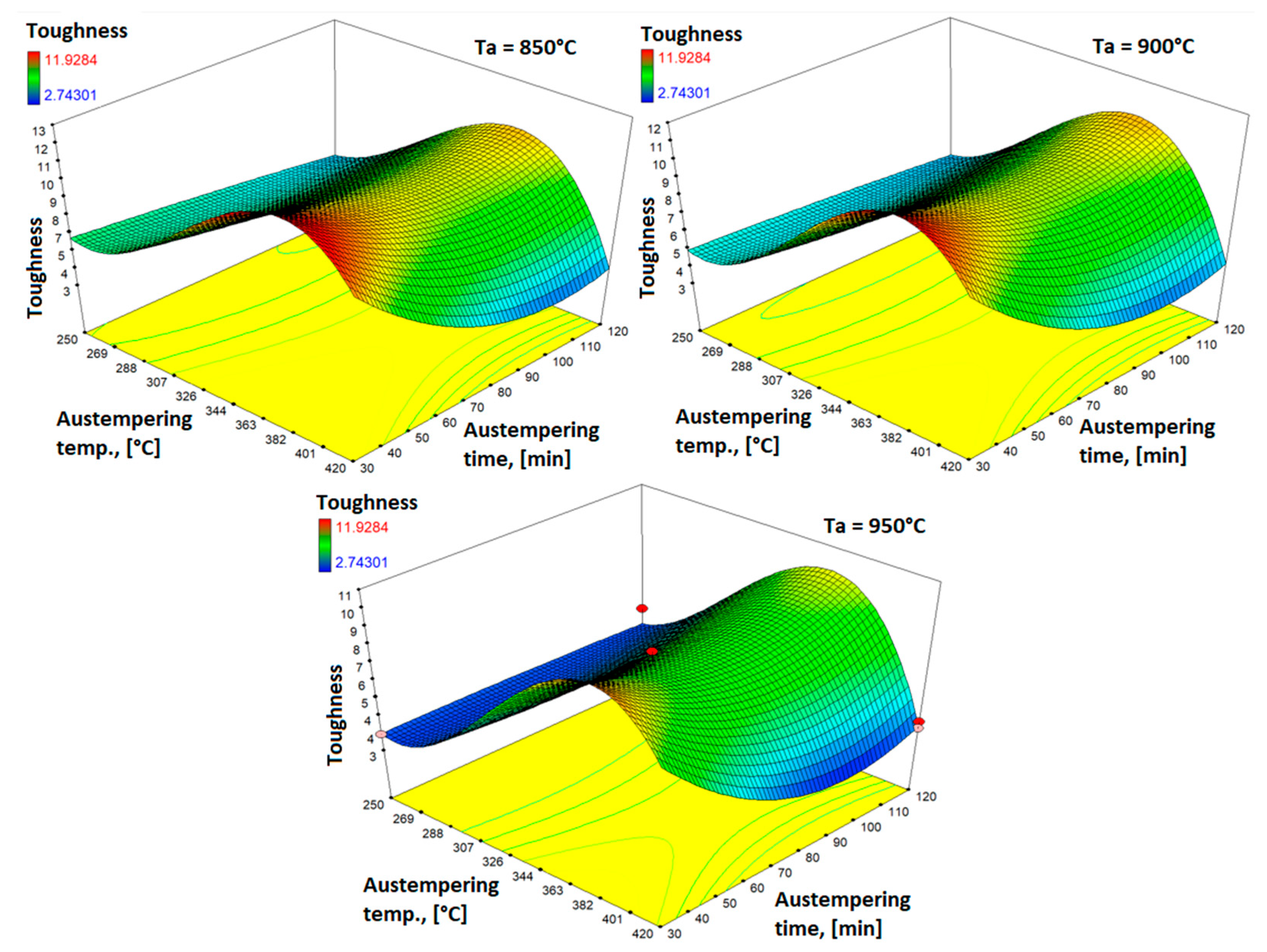
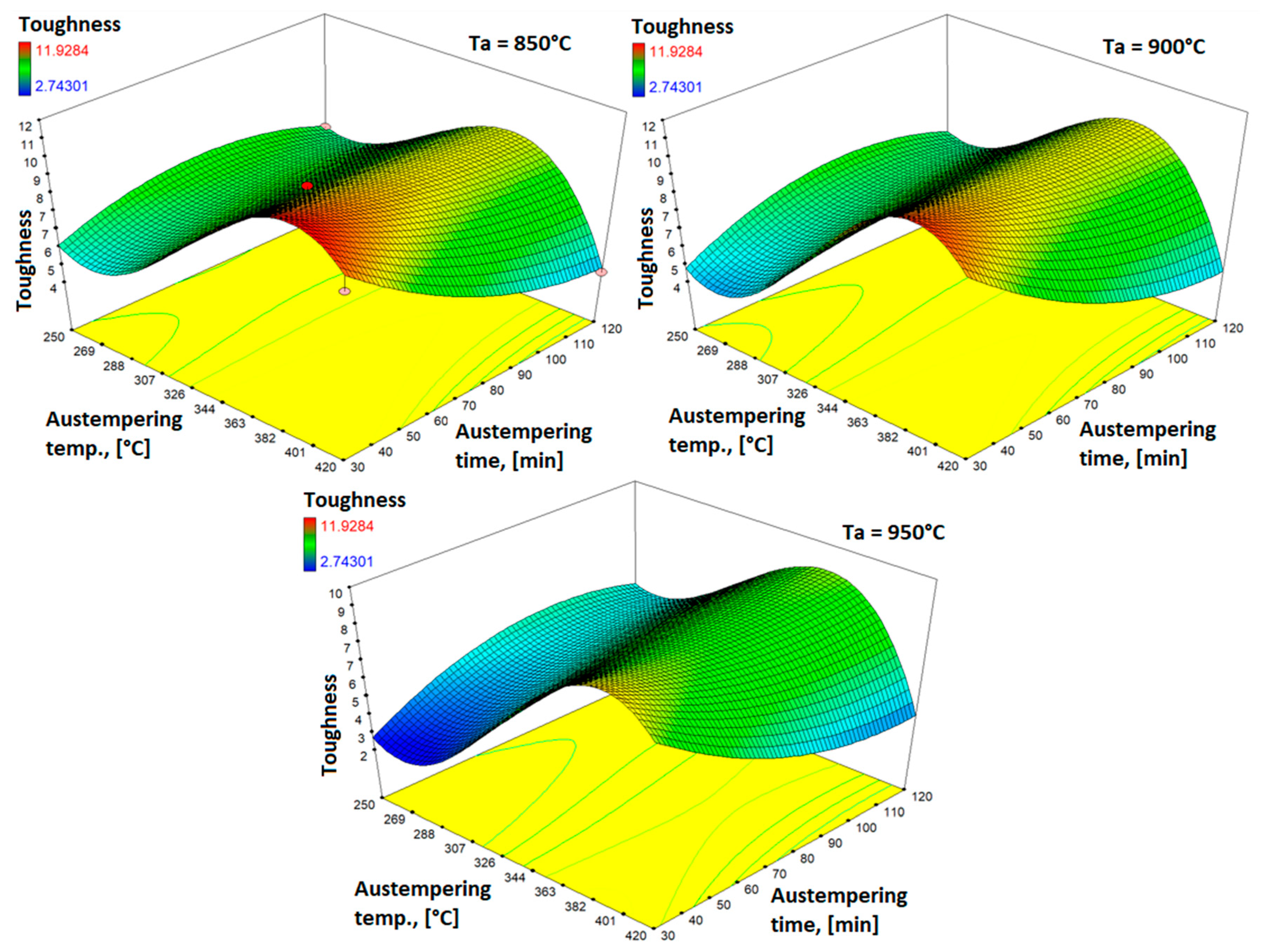
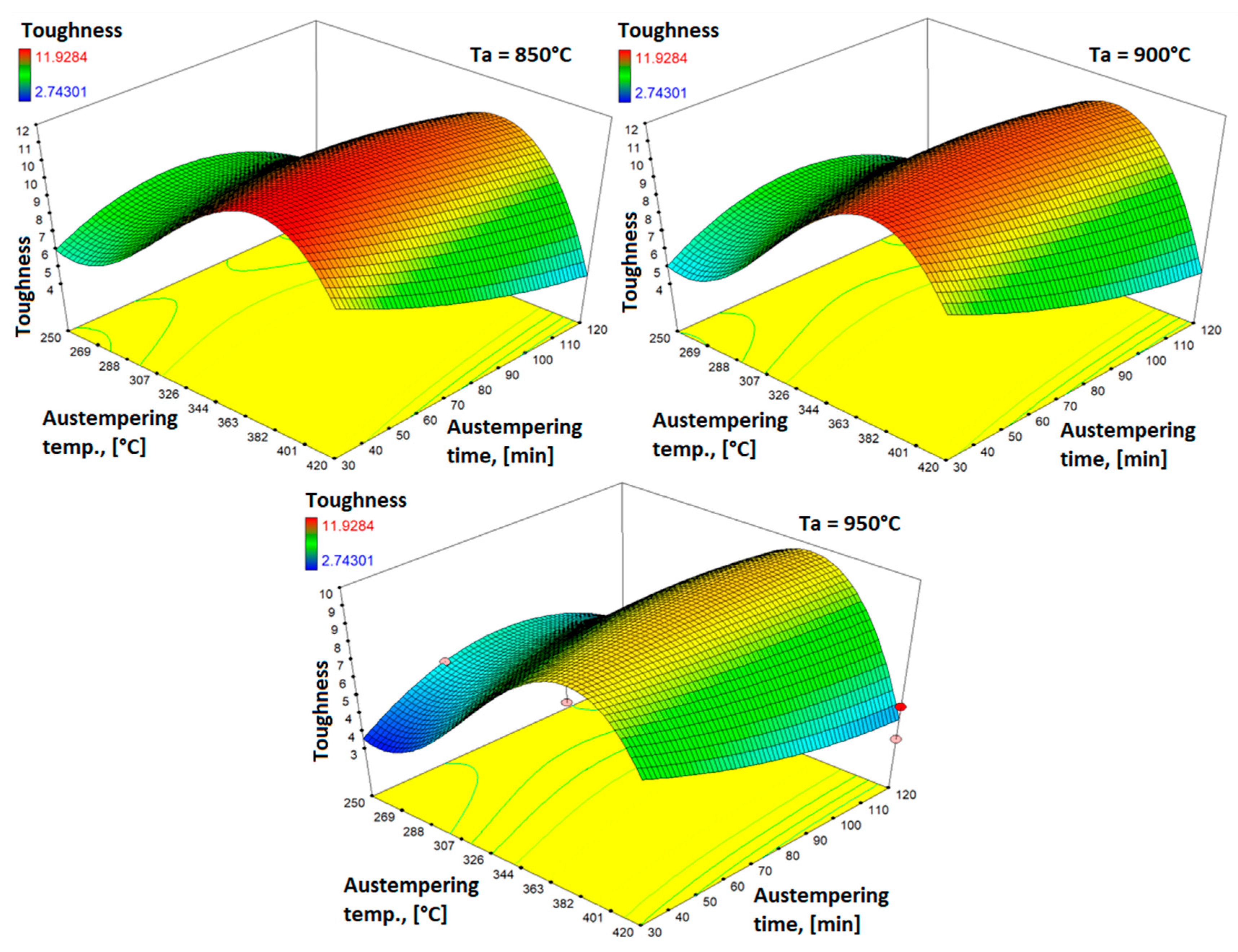
The toughness increases significantly as the austempering temperature rises up to a temperature of around 370 °C, and then decreases. The toughness is a qualitative indicator of the change in the volume fraction of retained austenite with the change in the austempering temperature. The high toughness values achieved with austempered samples at temperatures around 370 °C can be explained by the optimum retained austenite content in the microstructure of the test samples, which has been thoroughly explained in previous research [20].

-

At temperatures above 370 °C, the volume fraction of retained austenite decreases, as the ausferrite decomposes into ferrite and carbides during the second stage of ADI transformation, which leads to a deterioration of the mechanical properties.

-

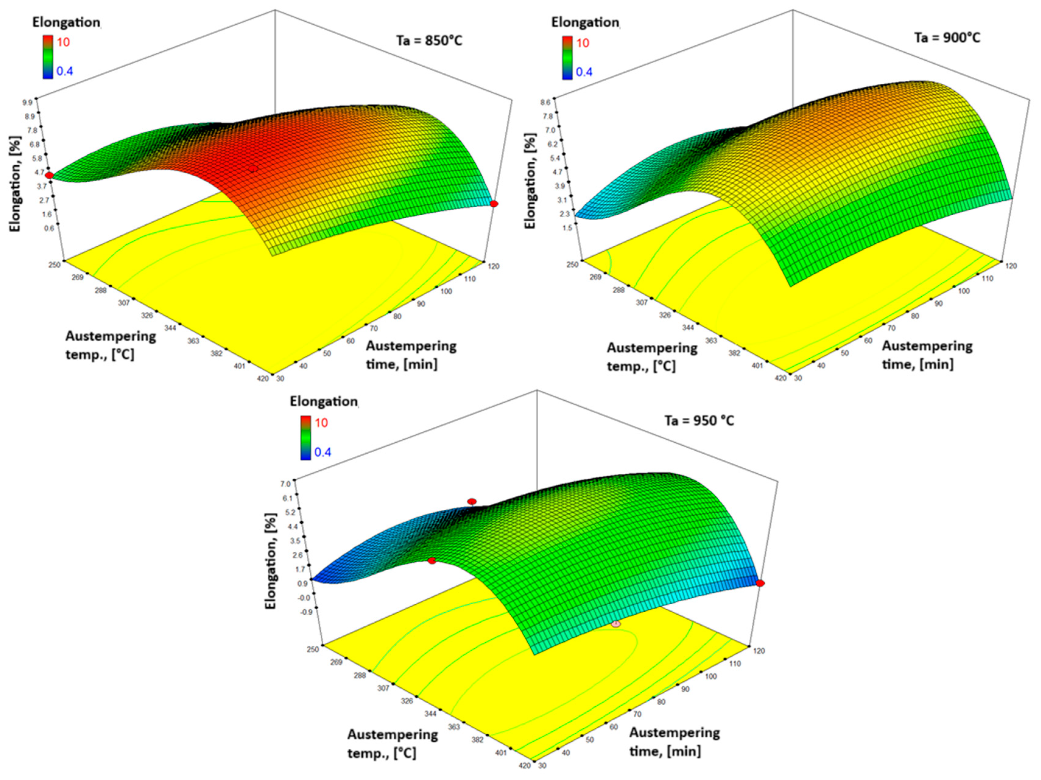
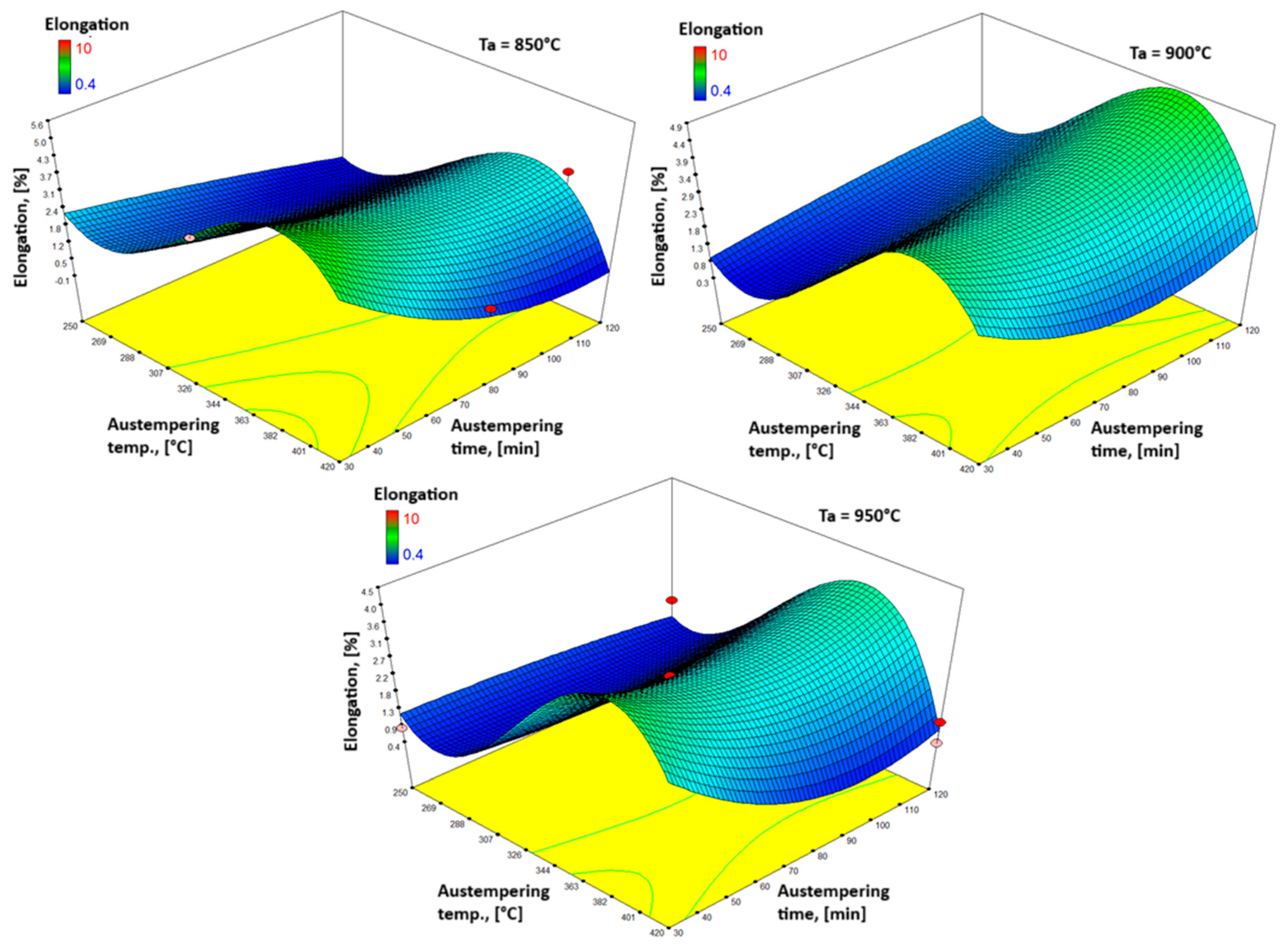
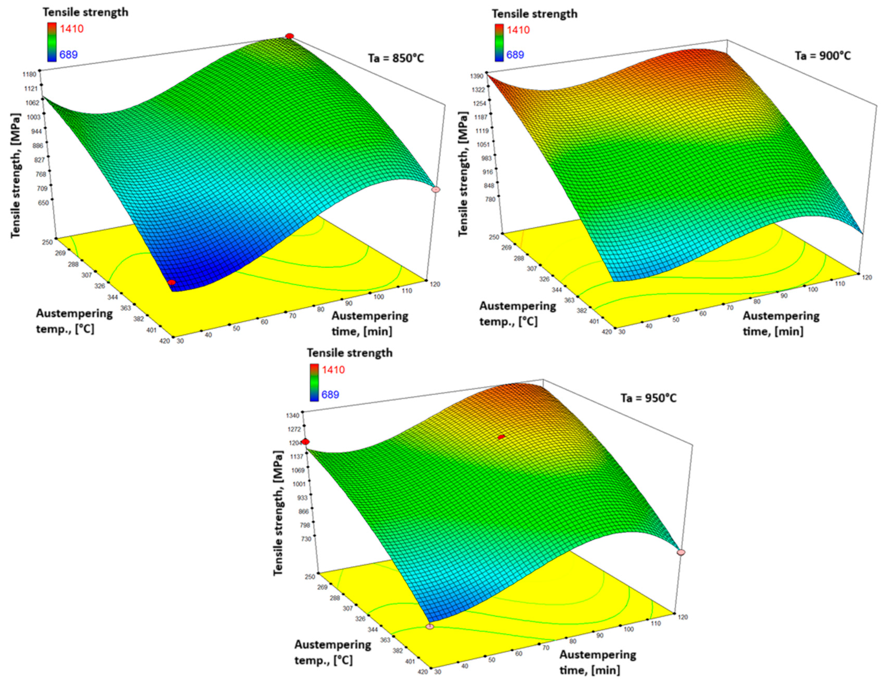
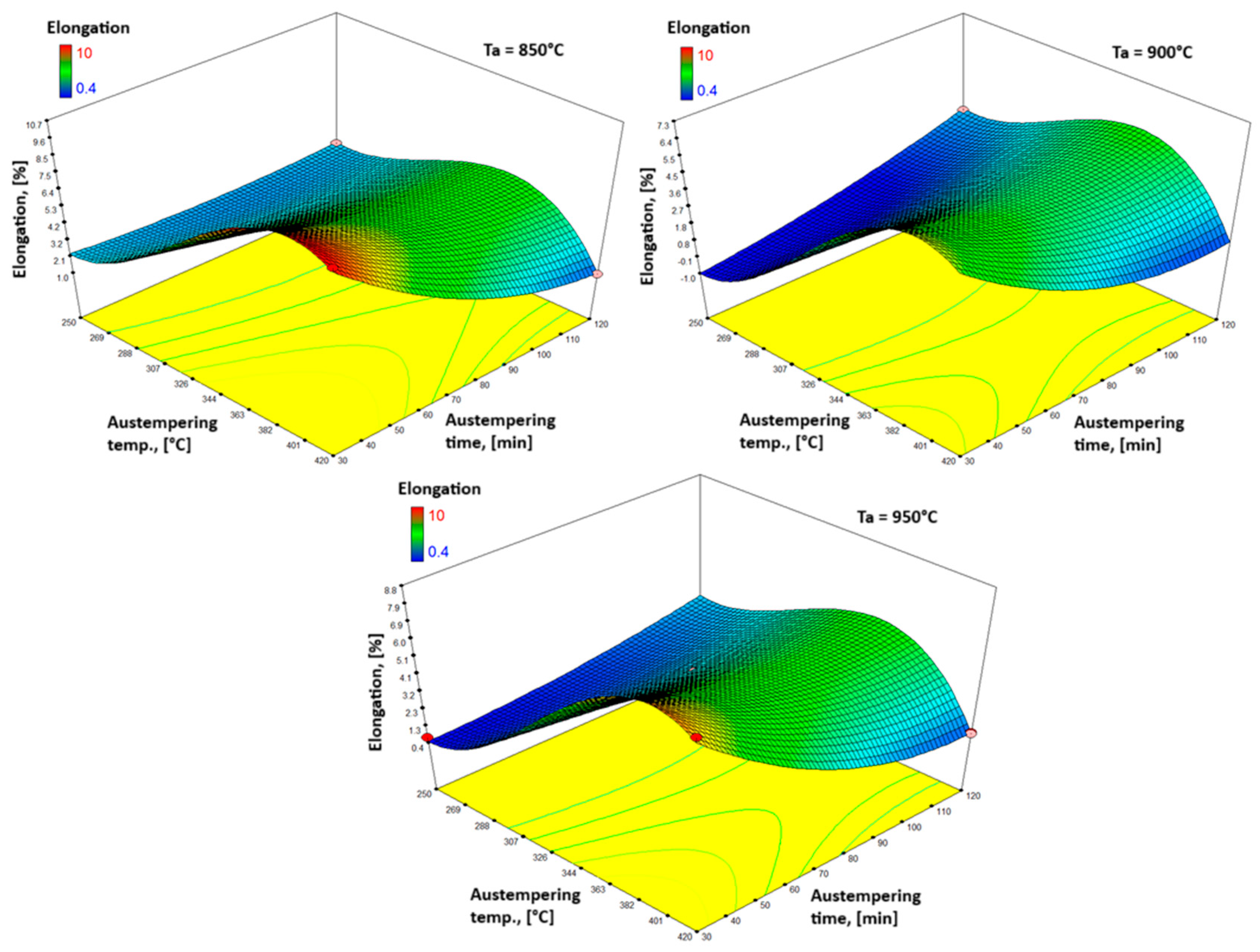
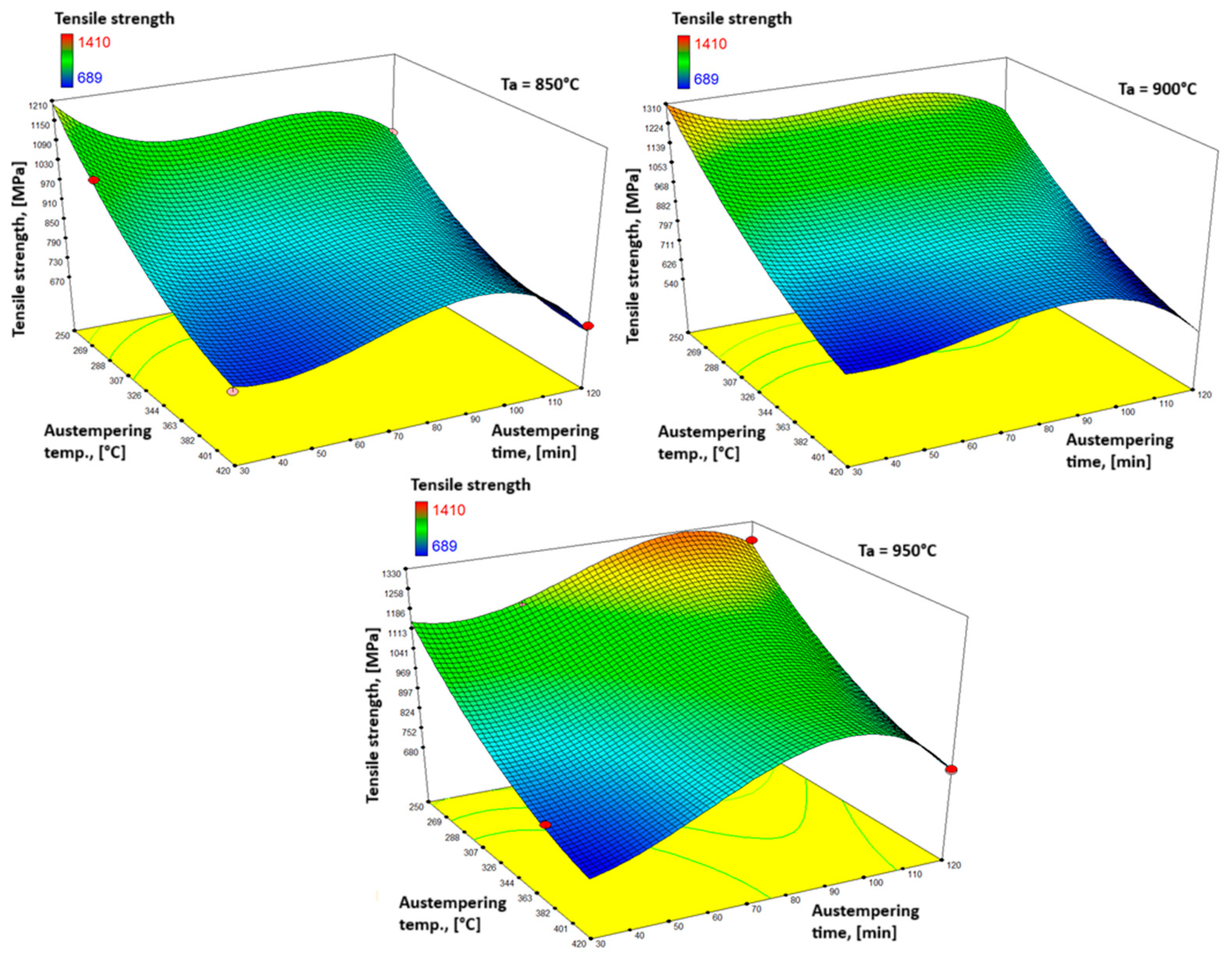
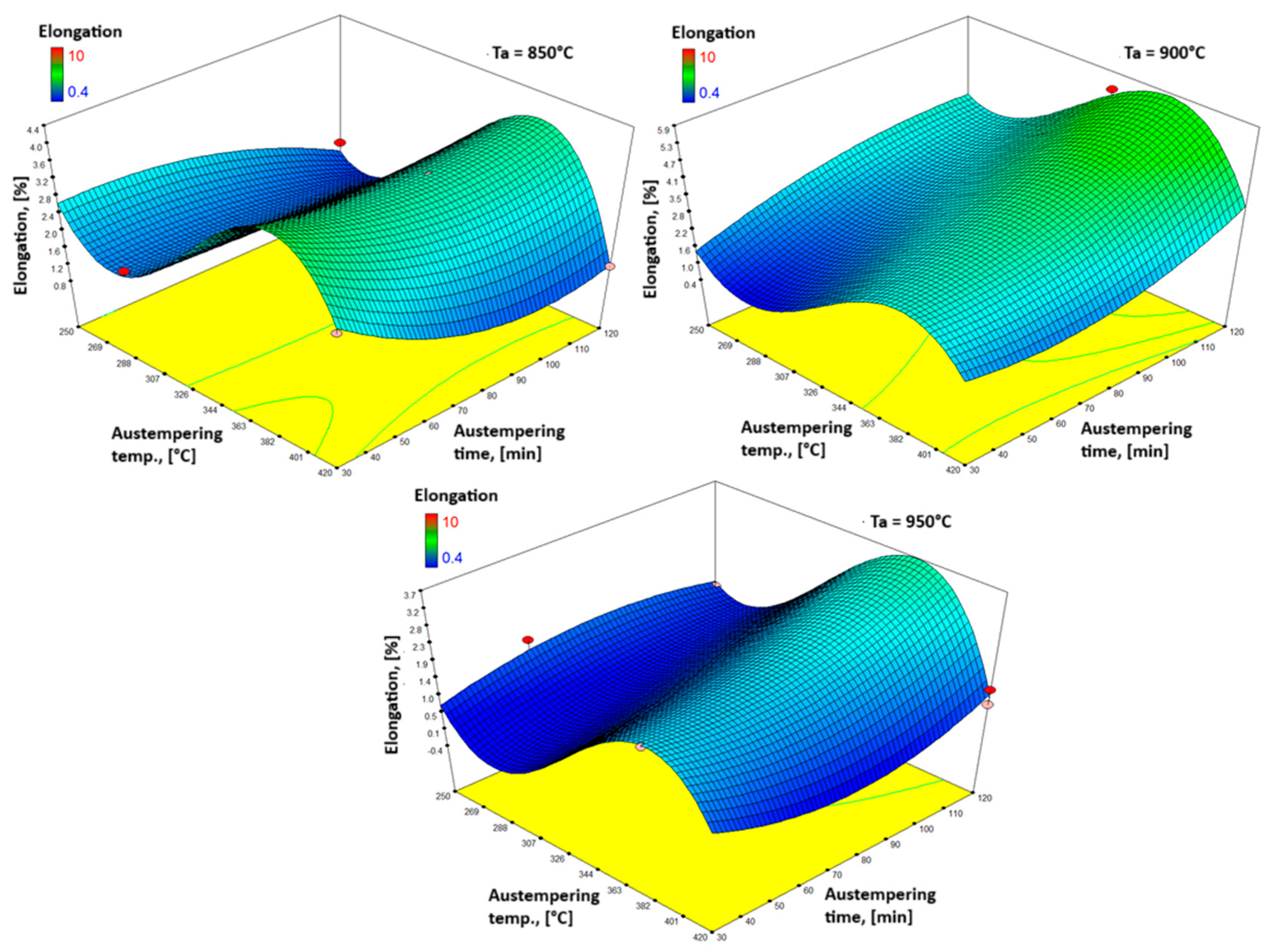
The tensile strength increases significantly with a longer austempering time but decreases as the austempering temperature increases. According to the figures shown in this paper, elongation increases with increasing austempering temperature. The increase can be observed up to a temperature of around 370 °C. Above the austempering temperature of 370 °C, the ductility decreases, qualitatively following the change in the volume fraction of the retained austenite.

-

The high elongation values achieved with samples that were austempered at temperatures around 370 °C can be explained by the optimum volume fraction of retained austenite in the microstructure of the test samples. At temperatures above 370 °C, the volume fraction of retained austenite decreases because the ausferrite decomposes into ferrite and carbides during the second transformation stage. This undesirable transformation leads to a deterioration in the mechanical properties.

-

It is clear from all the response surfaces shown that the toughness also increases with increasing copper content. This is a consequence of the richer initial microstructure of the ductile cast iron with pearlite and carbides, whose decomposition enriches the retained austenite during heat treatment and has a positive effect on toughness. In addition, the toughness decreases with increasing austenitizing temperature and austenitizing time.

-

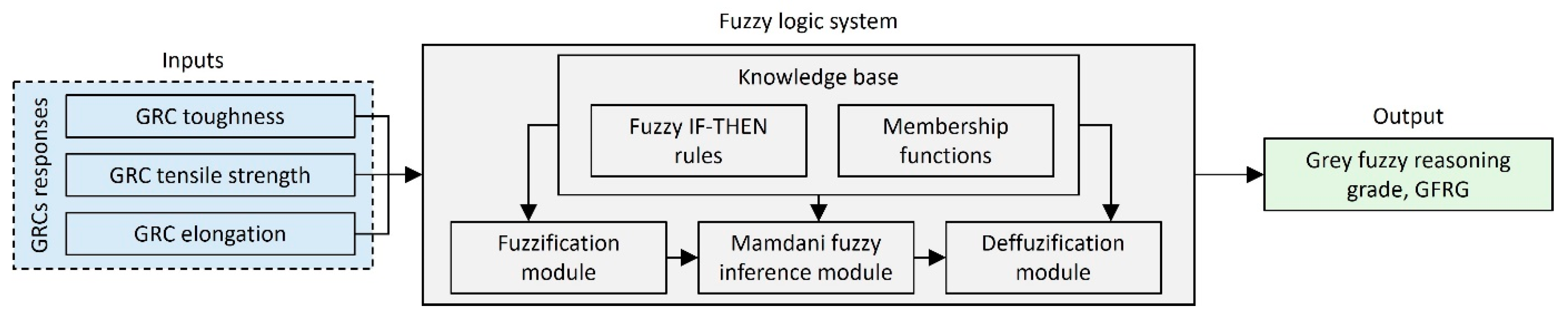
Due to the complexity of the investigated process and the dependencies of the experimental parameters on the mechanical properties, a comprehensive multi-response optimization was performed using the grey fuzzy technique. This technique proved to be a good solution to derive the parameter values that lead to maximum objective functions for the mechanical properties.

-

These input parameters, which correspond to the optimum result of the grey fuzzy optimization, are Austenitizing temperature: 850 °C, Austempering temperature: 384 °C, Austempering time: 42 min, Copper content: 0.031% Cu.

-

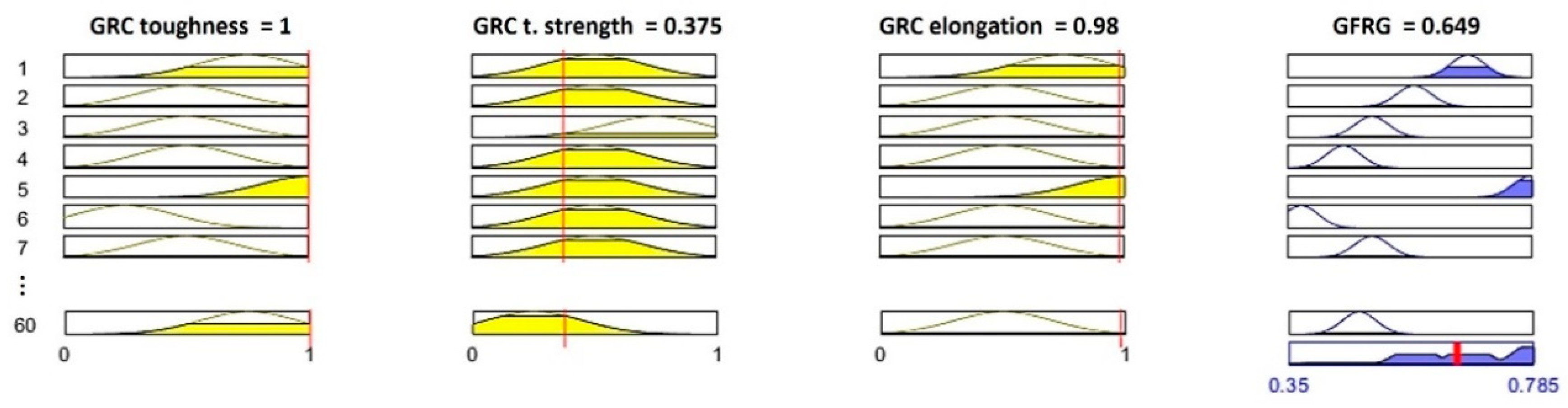
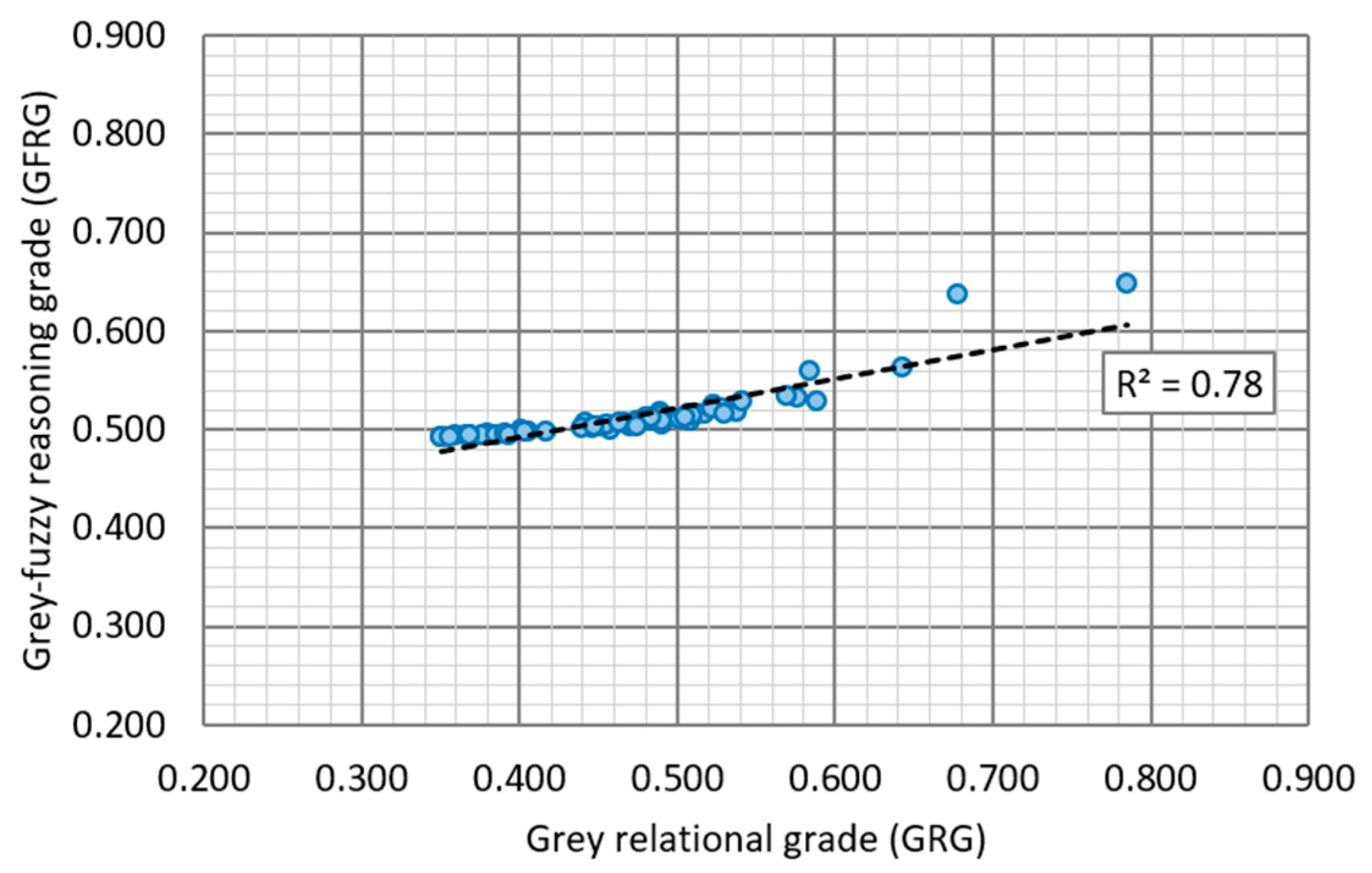
Apart from the fact that the fuzzy logic technique has proven to be a good extension of grey relational analysis, it has also proven to be a good tool to define relationships between experimental parameters and the Grey Fuzzy Reasoning Grade (GFGR).

-

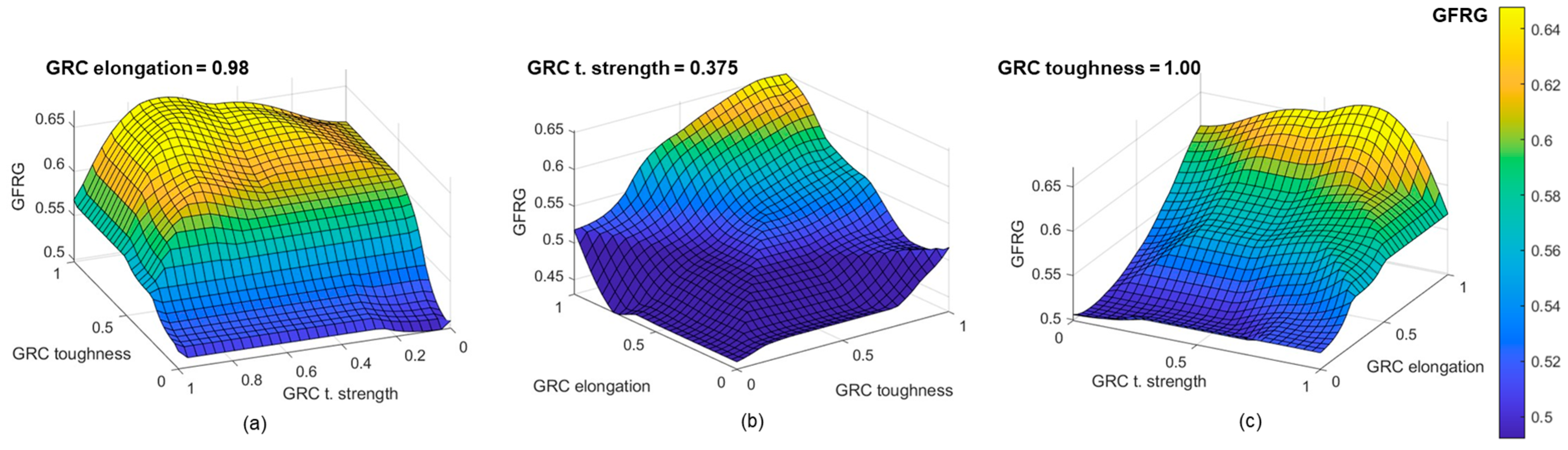
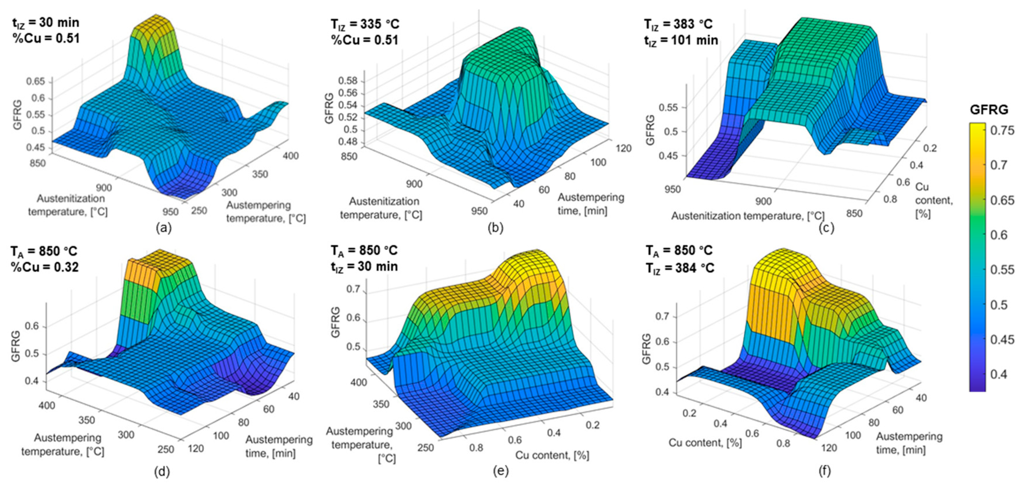
The GFRG transforms the multi-objective optimization into a single-objective optimization problem where the highest values of the GFRG are desirable. Based on the analysis of 3D response surface plots, which visualise the effects of the parameters on the GFRG values, the optimal ranges of parameter levels corresponding to the highest GFRG values were determined.

-

These derived parameter intervals are: Austenitizing temperature: 850–900 °C, austempering temperature: 380–420 °C, Austempering time: 30–50 min, Copper content: 0.031–0.51% Cu.

-

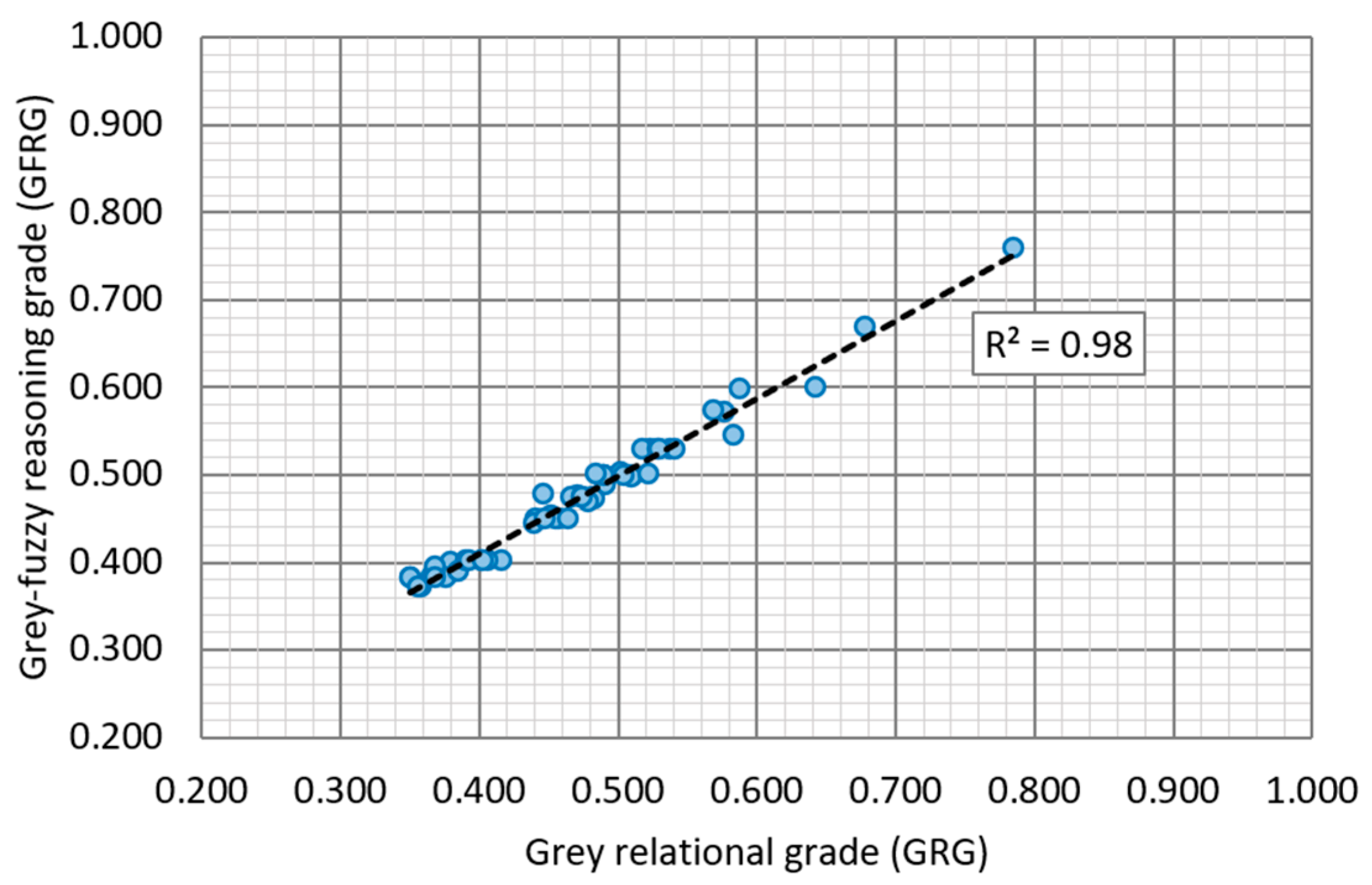
The quality of the fuzzy logic modelling was confirmed by validation measures such as the coefficient of determination (R²) and the mean absolute percentage error (MAPE). It can be concluded that the grey fuzzy technique can be successfully used to solve the problem of optimising the mechanical properties of several ADI alloys.

-

The findings obtained in this work are only valid within the range of the selected parameters. Further investigations in this area will focus on the implementation of additional experimental parameters as well as process reactions, which will then be subjected to further analysis and optimization.

-

Potential engineering application value of the presented work can be found in different industries. In general, ADI can be used in agriculture machinery, excavators, general application industry, gears, construction machinery, food industry, etc. The reason for this are favourable physical, mechanical and technological properties such as: resistance to corrosion, high modulus of elasticity, good castability, favourable strength, possibility of surface hardening, relatively good machinability and economic profitability.

References

1. Labercque, C.; Gagne, M. Ductile Iron—Fifty Years of Continued Development; Rio Tinto Iron & Titanium: Sorel-Tracy, QC, Canada, 1998. [Google Scholar]
2. Abdellah, M.Y.; Alharthi, H.; Alfattani, R.; Suker, D.K.; Abu El-Ainin, H.M.; Mohamed, A.F.; Hassan, M.K.; Backar, A.H. Mechanical Properties and Fracture Toughness Prediction of Ductile Cast Iron under Thermomechanical Treatment. Metals 2024, 14, 352. [Google Scholar] [CrossRef]
3. Behera, G.; Sohala, S.R. Effect of Copper on the Properties of Austempered Ductile Iron Castings. Bachelor’s Thesis, Department of Metallurgical and Materials Engineering, National Institute of Technology, Rourkela, India, 2012. [Google Scholar]
4. Čatipović, N.; Rogante, M.; Avdušinović, H.; Grgić, K. Influence of a Novel Double Tempering Process on the Microstructure and Mechanical Properties of Cu-Alloyed Austempered Ductile Iron with Possible Nano (Micro)-Characterization Using Neutron Beam Techniques. Crystals 2023, 13, 1359. [Google Scholar] [CrossRef]
5. Global Casting Production Trend and Conclusion in 2014. Available online: https://www.pinepacific.com/news_detail.php?idnews=93 (accessed on 2 August 2023).
6. Bendikiene, R.; Ciuplys, A.; Cesnavicius, R.; Jutas, A.; Bahdanovich, A.; Marmysh, D.; Nasan, A.; Shemet, L.; Sherbakov, S. Influence of Austempering Temperatures on the Microstructure and Mechanical Properties of Austempered Ductile Cast Iron. Metals 2021, 11, 967. [Google Scholar] [CrossRef]
7. Akinribide, O.J.; Ogundare, O.D.; Oluwafemi, O.M.; Ebisike, K.; Nageri, A.K.; Akinwamide, S.O.; Gamaoun, F.; Olubambi, P.A. A Review on Heat Treatment of Cast Iron: Phase Evolution and Mechanical Characterization. Materials 2022, 15, 7109. [Google Scholar] [CrossRef] [PubMed]
8. Sidjanin, L.; Smallman, R.E. Metallography of bainitic transformation in austempered ductile iron. Mater. Sci. Technol. 1992, 8, 1095–1103. [Google Scholar] [CrossRef]
9. Elliot, R. The role of research in promoting austempered ductile iron. Heat Treat. Met. 1997, 24, 55–59. [Google Scholar]
10. Landesberger, M.; Koos, R.; Hofmann, M.; Li, X.; Boll, T.; Petry, W.; Volk, W. Phase Transition Kinetics in Austempered Ductile Iron (ADI) with Regard to Mo Content. Materials 2020, 13, 5266. [Google Scholar] [CrossRef] [PubMed]
11. Tyrała, E.; Górny, M.; Kawalec, M.; Muszyńska, A.; Lopez, H.F. Evaluation of Volume Fraction of Austenite in Austempering Process of Austempered Ductile Iron. Metals 2019, 9, 893. [Google Scholar] [CrossRef]
12. Chandler, H. Heat Treaters Guide: Practices and Procedures for Irons and Steels, 2nd ed.; ASTM International: West Conshohocken, PA, USA, 1994. [Google Scholar]
13. Bai, J.; Xu, H.; Wang, Y.; Chen, X.; Zhang, X.; Cao, W.; Xu, Y. Microstructures and Mechanical Properties of Ductile Cast Iron with Different Crystallizer Inner Diameters. Crystals 2022, 12, 413. [Google Scholar] [CrossRef]
14. Hsu, C.-H.; Lin, C.-Y.; You, W.-S. Microstructure and Dry/Wet Tribological Behaviors of 1% Cu-Alloyed Austempered Ductile Iron. Materials 2023, 16, 2284. [Google Scholar] [CrossRef]
15. Sharma, A.; Singh, K.K.; Gupta, G.K. Study on the Effects of Austempering Variables and Copper Addition on Mechanical Properties of Austempered Ductile Iron. In Proceedings of the 6th International & 27th All India Manufacturing Technology, Design and Research Conference (AIMTDR-2016), Pune, India, 16–18 December 2016. [Google Scholar]
16. Wang, B.; Barber, G.C.; Qiu, F.; Zou, Q.; Yang, H. A review: Phase transformation and wear mechanisms of single-step and dual-step austempered ductile irons. J. Mater. Res. Technol. 2020, 9, 1054–1069. [Google Scholar] [CrossRef]
17. Liu, C.; Du, Y.; Wang, X.; Hu, Z.; Li, P.; Wang, K.; Liu, D.; Jiang, B. Mechanical and tribological behavior of dual-phase ductile iron with different martensite amounts. J. Mater. Res. Technol. 2023, 24, 2978–2987. [Google Scholar] [CrossRef]
18. Krawiec, H.; Lelito, J.; Mróz, M.; Radoń, M. Influence of Heat Treatment Parameters of Austempered Ductile Iron on the Microstructure, Corrosion and Tribological Properties. Materials 2023, 16, 4107. [Google Scholar] [CrossRef] [PubMed]
19. EN 1563:2018; Founding—Spheroidal Graphite Cast Irons. Croatia Standards Institute: Zagrzeb, Croatia, 2018. Available online: https://repozitorij.hzn.hr/norm/HRN+EN+1563%3A2018 (accessed on 2 August 2023).
20. EN ISO 6892; Metallic Materials—Tensile Testing—Part 1: Method of Test at Room Temperature. Croatia Standards Institute: Zagrzeb, Croatia, 2019. Available online: https://repozitorij.hzn.hr/norm/HRN+EN+ISO+6892-1%3A2019 (accessed on 2 August 2023).
21. EN ISO 148; Metallic Materials—Charpy Pendulum Impact Test—Part 1: Test Method. Croatia Standards Institute: Zagrzeb, Croatia, 2010. Available online: https://repozitorij.hzn.hr/norm/HRN+EN+ISO+148-1%3A2012 (accessed on 2 August 2023).
22. Design Expert 13 software, State-Ease. Available online: https://www.statease.com/training/quick-start-resources/ (accessed on 2 August 2023).
23. Čatipović, N.; Živković, D.; Dadić, Z.; Ljumović, P. Effect of Copper and Heat Treatment on Microstructure of Austempered Ductile Iron. Trans. Indian Inst. Met. 2021, 74, 1455–1468. [Google Scholar] [CrossRef]
24. Eric, O.; Sidjanin, L.; Miskovic, Z.; Zec, S.; Jovanovic, M.T. Microstructure and toughness of Cu, Ni Mo austempered ductile iron. Mater. Lett. 2004, 58, 2707–2711. [Google Scholar] [CrossRef]
25. Lapin, J.; Klimová, A.; Gabalcová, Z.; Pelachová, T.; Bajana, O.; Štamborská, M. Microstructure and mechanical properties of cast in-situ TiAl matrix composites reinforced with (Ti,Nb)2AlC particles. Mater. Des. 2017, 133, 404. [Google Scholar] [CrossRef]
26. Lapin, J.; Štamborská, M.; Pelachová, T.; Bajana, O. Fracture behaviour of cast in-situ TiAl matrix composite reinforced with carbide particles. Mater. Sci. Eng. A 2018, 721, 1–7. [Google Scholar] [CrossRef]
27. Ruggiero, A.; Khademi, E. Micromechanical Modeling for Predicting Residual Stress–Strain State around Nodules in Ductile Cast Irons. Metals 2023, 13, 1874. [Google Scholar] [CrossRef]
28. Lukic, D.; Cep, R.; Milosevic, M.; Antic, A.; Zivkovic, A.; Todic, V.; Rodic, D. A Grey Fuzzy Approach to the Selection of Cutting Process from the Aspect of Technological Parameters. Appl. Sci. 2022, 12, 12589. [Google Scholar] [CrossRef]
29. Sharma, A.; Kumar, V.; Babbar, A.; Dhawan, V.; Kotecha, K.; Prakash, C. Experimental Investigation and Optimization of Electric Discharge Machining Process Parameters Using Grey-Fuzzy-Based Hybrid Techniques. Materials 2021, 14, 5820. [Google Scholar] [CrossRef]
30. Babu, J.; Madarapu, A.; Paul, L.; Ahmed, A.N.K.; Davim, J.P. Multi-Response Optimization during the High-Speed Drilling of Composite Laminate Using the Grey Entropy Fuzzy Method (GEF). Processes 2022, 10, 1865. [Google Scholar] [CrossRef]
31. Das, B.; Roy, S.; Rai, R.N.; Saha, S.C. Application of grey fuzzy logic for the optimization of CNC milling parameters for Al–4.5%Cu–TiC MMCs with multi-performance characteristics. Eng. Sci. Technol. Int. J. 2016, 19, 857–865. [Google Scholar] [CrossRef]
32. Dragičević, M.; Begović, E.; Ekinović, S.; Peko, I. Multi-Response Optimization in MQLC Machining Process of Steel St50-2 Using Grey-Fuzzy Technique. Tech. Gaz. 2023, 30, 248–255. [Google Scholar]
33. Peko, I.; Nedić, B.; Dunđer, M.; Samardžić, I. Modelling of Dross Height in Plasma Jet Cutting Process of Aluminium Alloy 5083 Using Fuzzy Logic Technique. Tech. Gaz. 2020, 27, 1767–1773. [Google Scholar]
34. Lee, W.K.; Abdullah, M.D.; Ong, P.; Abdullah, H.; Teo, W.K. Prediction of flank wear and surface roughness by recurrent neural network in turning process. J. Adv. Manuf. Technol. 2021, 15, 55–67. [Google Scholar]
35. Hernández-Castillo, I.; Sánchez-López, O.; Lancho-Romero, G.A.; Castañeda-Roldán, C.H. An experimental study of surface roughness in electrical discharge machining of AISI 304 stainless steel. Ing. Investig. 2018, 38, 90–96. [Google Scholar] [CrossRef]
36. Peko, I.; Marić, D.; Nedić, B.; Samardžić, I. Modeling and Optimization of Cut Quality Responses in Plasma Jet Cutting of Aluminium Alloy EN AW-5083. Materials 2021, 14, 5559. [Google Scholar] [CrossRef]
Figure 1. Ductile iron ingot.
Metals 14 00735 g001
Figure 2. Ductile iron samples prepared for heat treatment.
Metals 14 00735 g002
Figure 3. Response surfaces for toughness of alloys with 0.031 wt.% Cu.
Metals 14 00735 g003
Figure 4. Response surfaces for toughness of alloys with 0.32 wt.% Cu.
Metals 14 00735 g004
Figure 5. Response surfaces for toughness of alloys with 0.51 wt.% Cu.
Metals 14 00735 g005
Figure 6. Response surfaces for toughness of alloys with 0.91 wt.% Cu.
Metals 14 00735 g006
Figure 7. Response surfaces for tensile strength of alloys with 0.031 wt.% Cu.
Metals 14 00735 g007
Figure 8. Response surfaces for elongation of alloys with 0.031 wt.% Cu.
Metals 14 00735 g008
Figure 9. Response surfaces for tensile strength of alloys with 0.32 wt.% Cu.
Metals 14 00735 g009
Figure 10. Response surfaces for elongation of alloys with 0.32 wt.% Cu.
Metals 14 00735 g010
Figure 11. Response surfaces for tensile strength of alloys with 0.51 wt.% Cu.
Metals 14 00735 g011
Figure 12. Response surfaces for elongation of alloys with 0.51 wt.% Cu.
Metals 14 00735 g012
Figure 13. Response surfaces for tensile strength of alloys with 0.91 wt.% Cu.
Metals 14 00735 g013
Figure 14. Response surfaces for elongation of alloys with 0.91 wt.% Cu.
Metals 14 00735 g014
Figure 15. Architecture of fuzzy logic system for modelling relations between responses GRCs and GFRG.
Metals 14 00735 g015
Figure 16. Gaussian membership functions for: (a) input: GRC toughness and (b) output: GFRG.
Metals 14 00735 g016
Figure 17. Fuzzy IF-THEN rules viewer for defined inputs and corresponding GFRG.
Metals 14 00735 g017
Figure 18. GFRG results for the experimental trials.
Metals 14 00735 g018
Figure 19. Comparison between calculated GRG and predicted GFRG.
Metals 14 00735 g019
Figure 20. 3D surface plots of GRC mechanical properties responses: (a) toughness and tensile strength, (b) elongation and toughness, (c) tensile strength and elongation effects on GFRG values.
Metals 14 00735 g020
Figure 21. Gaussian membership functions for parameters: (a) austenitization temperature, (b) austempering temperature, (c) austempering time, (d) copper content.
Metals 14 00735 g021aMetals 14 00735 g021b
Figure 22. Comparison between calculated GRG and predicted GFRG.
Metals 14 00735 g022
Figure 23. 3D surface plots of parameters effects: (a) austenitization temperature and austempering temperature, (b) austenitization temperature and austempering time, (c) austenitization temperature and Cu content, (d) austempering temperature and austempering time, (e) austempering temperature and Cu content, (f) Cu content and austempering time on GFRG values.
Metals 14 00735 g023