Abstract
Due to the scarcity of modeling samples and the low prediction accuracy of the matte grade prediction model in the copper melting process, a new prediction method is proposed. This method is based on enhanced generative adversarial networks (EGANs) and random forests (RFs). Firstly, the maximum relevance minimum redundancy (MRMR) algorithm is utilized to screen the key influencing factors of matte grade and remove redundant information. Secondly, the GAN data augmentation model containing different activation functions is constructed. And, the generated data fusion criterion based on the root mean squared error (RMSE) and the coefficient of determination (R2) is designed, which can tap into the global character distributions of the copper melting data to improve the quality of the generated data. Finally, a matte grade prediction model based on RF is constructed, and the industrial data collected from the copper smelting process are used to verify the effectiveness of the model. The experimental results show that the proposed method can obtain high-quality generated data, and the prediction accuracy is better than other models. The R2 is improved by at least 2.68%, and other indicators such as RMSE, mean absolute error (MAE), and mean absolute percentage error (MAPE) are significantly improved.
1. Introduction
Isa furnace copper smelting is one of the main methods of modern thermal copper refining. In the smelting process, matte grade is a critical process indicator for measuring the quality of the smelting process and can guide the adjustment of operating parameters []. A stable matte grade plays a vital role in the subsequent blowing, electrolysis, and sulfuric acid production processes. However, due to the complexity of the Isa furnace melting reaction mechanism, the solid phase, liquid phase, and gas phase coexist in the furnace, resulting in an inability to achieve the real-time detection of matte grade. Existing approaches mostly adopt laboratory testing to detect the value of the matte grade, which results in an inability to adjust the operating parameters in a timely manner []. Therefore, constructing an accurate and effective prediction model for matte grade is of great significance in guiding the production operation of copper melting processes.
The available research mainly inputs the production parameters of the copper smelting process into a data-driven model that can achieve the prediction of matte grade. Shouyi Yu et al. [] proposed a prediction method for matte grade, matte temperature, and iron–silicon ratio in slag in the copper smelting process based on an artificial neural network and achieved the real-time prediction of three main process parameters in the copper smelting process. Weihua Gui et al. [] constructed a matte grade prediction model based on a fuzzy neural network and improved the gradient descent algorithm to enhance the accuracy of matte grade prediction. Chunhua Yang et al. [] proposed an intelligent integrated prediction model for matte grade and verified the effectiveness of the model using industrial data. Xiaobo Peng et al. [] established a dynamic T-S recursive fuzzy neural network prediction model and applied it to the prediction of key parameters in the copper flash melting process. Jianhua Liu et al. [] proposed a prediction method for key process indicators of the copper flash melting process based on projection seeking regression, utilizing an accelerated genetic algorithm for updating model parameters in real time. Xiaolong Zhang et al. [] proposed an adaptive Isa furnace copper melting process prediction method based on generalized maximum entropy regression to improve the prediction accuracy. Maoqi He et al. [] proposed a data-driven modeling method based on the soft measurement of matte grade and predicted matte grade during oxygen-enriched side-blowing melt pool melting. The above matte grade prediction methods mainly integrate traditional machine learning methods to learn the mapping relationship between input variables and matte grade from historical data, so as to predict unknown data. However, in the actual production process of copper smelting, an offline analysis of ore composition and matte grade take a lot of time and money, which leads to the scarcity of modeling samples and limits the development of matte grade prediction technology.
To address the above problem, scholars have proposed data augmentation methods such as geometric transformation, window clipping, adding noise [], FBG [], and generative adversarial networks (GANs) []. In particular, a generative adversarial network (GAN) can learn high-dimensional and complex data distributions without relying on any prior assumptions, which have a wide range of applications in complex industrial fields. Zherui Ma et al. [] proposed a virtual sample generation method based on GAN, which improved the accuracy of hydrogen yield prediction during supercritical water gasification hydrogen production. Xiaochen Hao et al. [] proposed a data augmentation model of calcium oxide in a cement clinker based on the Wasserstein generative adversarial network (WGAN), which solved the problem of low prediction accuracy caused by limited labeled samples. Zhongsheng Chen et al. [] proposed an industrial data generation method based on the conditional generative adversarial network (CGAN), which improved the performance of soft measurement models. Yajun Wu et al. [] combined WGAN with the Gradient Penalty and Extreme Gradient Boosting Algorithm, which expanded the experimental data and established the relationship between the process parameters and relative density of aluminum alloy thin-walled parts. And, the influence of process parameters on the relative density was revealed. Zhongsheng Chen et al. [] proposed a data augmentation method for embedding quantile regression into CGAN and verified the effectiveness of the proposed method through chemical data. Zoujing Yao et al. [] proposed a generative adversarial data filling model with the addition of a soft measurement module, and verification of the proposed method was accomplished with the collected chemical data.
In summary, GAN-based augmentation methods provide a new research direction for matte grade prediction under limited data. However, a GAN with a single activation function cannot fully represent the positive and negative characteristics of copper melting data, resulting in a large distribution discrepancy between the generated data and real data, which reduces the prediction model’s performance. For this reason, a novel matte grade prediction method considering limited data is proposed. The main contributions of this paper are summarized as follows:
- To select the most relevant and the least redundant variable subsets, a maximum relevance minimum redundancy (MRMR) algorithm is introduced to screen the variables, which ensures that the selected variables can effectively capture the change pattern of the matte grade and reduce redundant information.
- Three GAN data augmentation models with different activation functions are constructed, and a data fusion criterion generated based on the root mean squared error (RMSE) and the coefficient of determination (R2) is designed, which can improve the global features’ ability to represent a generative network and the quality of the generated data.
- A matte grade prediction model based on GANs and random forest (RF) is proposed. The prediction method is verified by the production data of a copper smelting enterprise in southwest China. The experimental results show that the proposed method has high prediction accuracy.
2. Theory and Methodology
2.1. Maximum Correlation Minimum Redundancy Algorithm
The maximum relevance minimum redundancy (MRMR) algorithm can maximize the correlation between the input variables and the target variables and minimize the correlation between the input variables simultaneously [].
Assuming that the joint probability density function p(x,y) and the marginal probability density function p(x), p(y) between two variables are known, the expression for the mutual information is shown in Equation (1).
Assuming that S is the optimal subset of input variables and |S| is the number of variables in S, the maximum correlation can be defined as Equation (2).
However, there is a redundancy issue among the variables based on maximum correlation. Therefore, a minimum redundancy constraint is introduced, as shown in Equation (3).
Combining these two constraints, the maximum correlation minimum redundancy can be obtained. The expression is shown in Equation (4).
Assuming that the set of all variables is X, the set of selected variables is Sm−1, where there are m − 1 variables. The incremental search method is used to select the mth variable from the remaining variable set X-Sm−1, which needs to meet the requirements of Equation (4). The expression can be shown in Equation (5).
2.2. The Principle of GAN
The structure of GAN is shown in Figure 1, which mainly consists of a generator and a discriminator [].
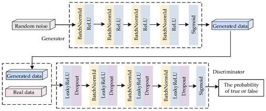
Figure 1.
Generative adversarial network structure.
During training, the generator is responsible for learning the distribution mapping of real data, and its output is shown in Equation (6).
where φG denotes the activation function of the generator; z denotes the random noise sample; and WG and bG denote the weights and biases in the generator.
When the input is a real sample, the output of the discriminator is 1; when the input is a pseudo-sample, the output of the discriminator is 0, as shown in Equations (7) and (8).
where φD denotes the activation function of the discriminator; x denotes a real data sample; and WD and bD denote the weights and biases in the discriminator.
The entire training process of GAN can be regarded as a binary minimax game problem, as shown in Equation (9).
where P(x) denotes the true data distribution; Pz(z) denotes the distribution of noise; and E denotes the expected value.
2.3. RF Model
RF has been widely applied in nonlinear regression prediction []. Assuming that the number of samples in the training set is X and the number of variables is M, the process of prediction using the RF model is shown in Figure 2.
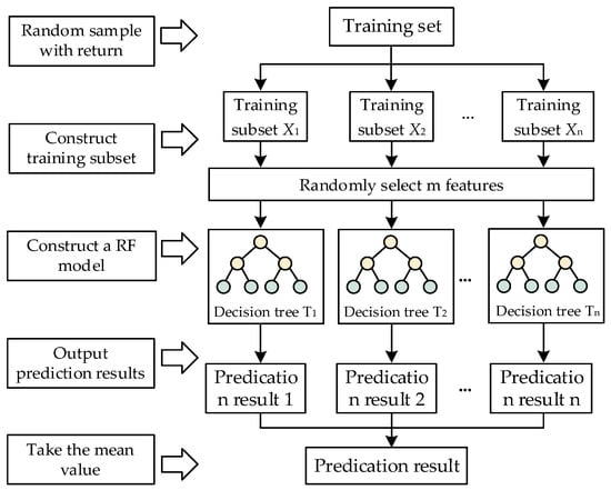
Figure 2.
RF model prediction flowchart.
- A training subset is constructed by randomly selecting x samples from the original training set. And, m variables are randomly selected from the training subset, and the corresponding decision tree is constructed.
- Repeating step (1) n times, a total of n training subsets are obtained, forming n decision trees, and all the decision trees are combined together to obtain an RF model.
- The predictions of all the decision trees were averaged as the final prediction of the random forest regression model.
3. A Matte Grade Prediction Model Incorporating EGAN and RF
The overall architecture of the model is shown in Figure 3. The most valuable information for the prediction task is retained through the MRMR algorithm. The generated data closer to the real data distribution is obtained through GANs and data fusion, and the predicted value of the matte grade is obtained via the RF model.
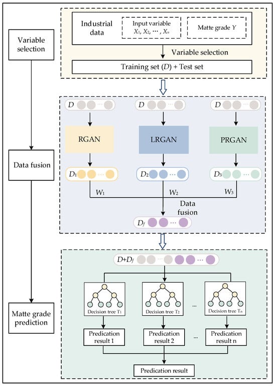
Figure 3.
Overall framework of the matte grade prediction model, fusing the generative adversarial network and random forest.
3.1. Variable Selection Based on MRMR Algorithm
The data in this paper come from the production data of a copper smelting enterprise in southwestern China. And, 17 variables were selected as inputs to the prediction model. Based on the chemical reaction mechanism of copper melting, the 17 variables were categorized into positively and negatively correlated variables, as shown in Table 1.

Table 1.
Input variables for matte grade prediction model.
The MRMR algorithm was applied to select the key variables of matte grade prediction and reduce the influence of redundant variables on the prediction model. Its specific process can be explained as follows:
- The variable Xj is selected from the input variable set X that has the maximum mutual information with the matte grade and placed into the optimal input variable subset S.
- The incremental search method is used to select the variable Xj that satisfies the condition and place it into the optimal input variable subset S.
- Whether the set threshold reached (ψ(D,R) > 0) is determined. If the threshold condition is met, the selected variable is output; otherwise, the second step is performed.
3.2. Data Augmentation and Data Fusion Based on GANs
In the process of matte grade prediction, we have selected many positive correlation variables and negative correlation variables to improve the prediction accuracy, as shown in Table 1. When constructing the generative model, accurately representing the variables features is a significant way to improve the quality of the generated data.
Activation functions are crucial to represent variables features for GANs. Specifically, compared to Sigmoid, Tanh, and Softmax activation functions, ReLU can speed up model training and effectively solve the problem of gradient vanishing. The ReLU activation function is widely used in GAN []. However, ReLU lacks the ability to represent negative features, which makes the generator unable to learn the global features of real data, resulting in a decline in the quality of generated data.
For this reason, relevant scholars have introduced LeakyReLU [] and PreLU [] activation functions into the generator and introduced negative slopes on the basis of ReLU, which can assist the generator to characterize negative features.
The diversity of activation functions has a significant impact on the generator in characterizing data features. In this paper, a comprehensive strategy using multiple activation functions is proposed, which can capture the global variable characteristics of the copper melting data. And, three different activation functions are utilized for data generation, as shown in Table 2.
Table 2.
GAN models with different combinations of activation functions.
According to the data fusion method in Reference [], the three kinds of data are weighted and fused, as shown in Equations (10)–(12).
where RMSEi and R2i represent the root mean square error and the coefficient of determination, respectively. Ci represents the quadratic evaluation index based on the RMSEi and R2i, and the larger the value of Ci, the higher the prediction accuracy of the model. Di and wi represent the different generated data and their corresponding weights, Df represents the weighted fusion data, and m represents the number of different GAN models used.
The generated data are used as the extended data of the training set and then input into the RF model to obtain the corresponding RMSE and R2 and update the weights of the generated data. The data fusion based on RMSE and R2 can obtain new generated data. The steps for data fusion are as follows:
- The key influencing variables of matte grade were obtained by using the MRMR algorithm for variable selection, which was divided into a training set and a test set in the ratio of 8:2.
- The training set D was input into the RGAN model, and the generated data D1 under RGAN were obtained according to a ratio of real data to generated data of 1:1.
- The generated data D1 obtained under the RGAN model were used as the extended data of training set D and fed into the RF model, and the evaluation metrics C1 was computed.
- Steps (2) and (3) were repeated following the same method to obtain the generated data D2 and D3 under LRGAN and PRGAN, respectively, as the extended data for training set D. Then, they were input into the RF model and evaluation indexes C2 and C3 were computed sequentially.
- Weights w1, w2, and w3, corresponding to each GAN model’s generated data, and the weighted fusion of the three generated data were calculated to obtain the final generated data Df.
3.3. Matte Grade Prediction Based on Random Forest
The generated data after weighted fusion were used as the extended data of the real training data to obtain new training data. The new training data were then input into the RF prediction model for model training, and finally, the random forest prediction model with the smallest generalization error was obtained and the trained model was used to predict the data in the test set by adding the prediction results of each decision tree and then taking the average value as the final matte grade prediction, as shown in Equation (13).
where F(x) is the final matte grade prediction result and fi(x) is the matte grade prediction result of the ith decision tree.
4. Experimental Results and Analysis
4.1. Data Sources and Experimental Settings
4.1.1. Copper Smelting Mechanism and Data Sources
The acquisition of the copper concentrate is the primary step. Firstly, the copper ore mined from the mine is crushed and ground. Secondly, the broken ore is separated following a flotation process to extract copper-containing minerals and form the copper concentrate. Then, the copper concentrate is concentrated and dried to increase its copper content and remove excess water. Finally, a copper concentrate with a high copper content is obtained for subsequent Isa furnace smelting.
The top-blowing smelting of the Isa process is a key link in the copper smelting process, and the process is shown in Figure 4. The concentrate raw materials, coal, slagging agent, and flux are mixed and added to the molten pool through the furnace top feeding port. Meanwhile, the spray gun is inserted into the molten pool, and the oxygen-enriched air and diesel oil are blown into the molten pool through the spray gun. The solid, liquid, and gas phases are fully mixed and stirred in the molten pool through the entrainment effect, so that the copper concentrate undergoes a chemical reaction to generate heat and maintain the high-temperature environment in the furnace. Finally, matte and slag enter the depleted electric furnace in the form of molten mixing to achieve the separation of copper and slag []. The main chemical reaction equations in the Isa furnace are as follows.
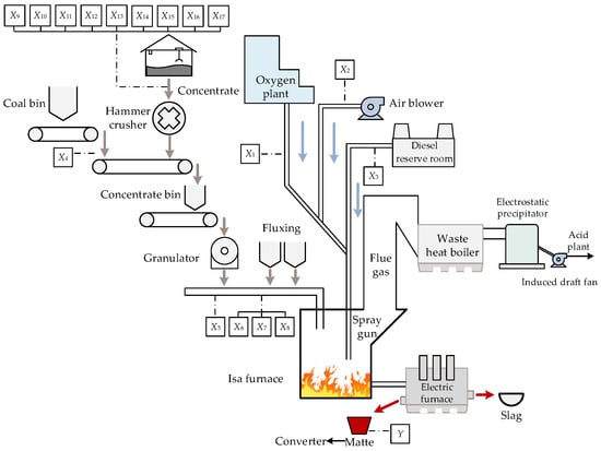
Figure 4.
Isa furnace melting process flow diagram.
- 1.
- Decomposition reaction of sulfides. The main components of copper concentrate are CuFeS2, CuS, FeS2, etc. After the copper concentrate enters the Isa furnace, the decomposition reaction of high-valence sulfides occurs rapidly, as shown in Equations (14)–(16).The FeS and Cu2S produced by the decomposition of the above sulfides will continue to be oxidized or form copper matte, and the resulting S2 will continue to be oxidized into SO2 into the flue gas, as shown in Equation (17).
- 2.
- Oxidation reaction of sulfides. In the Isa furnace, in addition to the decomposition reaction, the sulfide will be directly oxidized, the oxidation reaction will occur, and some will be reduced to high-valence oxides, as shown in Equations (18)–(22).
- 3.
- Reaction between sulfides and oxides. The oxidation reaction in the Isa furnace is intense, and the reaction product will contain a small amount of Cu2O and Fe3O4. In the separation process of matte and slag in the electric furnace, the sulfide in the matte will further react with the metal oxide in the slag, as shown in Equations (23) and (24).
- 4.
- Slagging reaction. The impurities in the molten copper are removed by adding a slagging agent to produce a slagging reaction, as shown in Equations (25) and (26).
The data in this paper come from the production data of a copper smelting enterprise in southwestern China. The input variables are listed in Table 1. And, 1136 sets of data were obtained. Among them, the first 909 sets of data were selected as the training datasets, and the last 227 sets of data were used as the test datasets.
4.1.2. Model Parameter Settings
The parameter settings of the GAN and RF models are crucial for the performance of the models. The parameters of GAN and RF used in this article are shown in Table 3 and Table 4. The experiments were implemented in Python 3.9.7 and PyTorch 1.9.1 with the CUDA 11.2 environment running on a computer with Intel (R) Core (TM) i7-10875H CPU @ 2.30 GHz (8CPUs, NVIDIA GeForce RTX 2060, manufacturer: NVIDIA corporation, Santa Clara, CA, USA) processor, 3.4 GHz 64 G RAM. And, the proposed model uses machine learning libraries such as NumPy, Pandas, and Matplotlib.
Table 3.
GAN model parameters.
Table 4.
RF model parameters.
4.2. Data Preprocessing and Variable Screening
The original data collected from the industrial site have outliers and missing values, and the data need to be preprocessed to improve the data quality. Firstly, in order to avoid the influence of different dimensions of data, the data were normalized, as shown in Equation (27). Secondly, a box plot was used to screen out outliers in the data. The results of the box plot to screen out outliers are shown in Figure 5. Finally, the interpolation method was used to fill the missing values in the data.
where x denotes the data to be normalized; xmin and xmax denote the minimum and maximum values of x, respectively; and denotes the value after normalization.
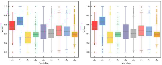
Figure 5.
The box plot screens out the outliers in the data.
Using the MRMR algorithm, 12 key variables required for predicting matte grade were chosen: X1, X2, X3, X4, X5, X6, X9, X10, X11, X12, X15, X16. X7, and X8 were not selected, probably because X6 is sufficient to characterize the main components of the flux silicon, resulting in high redundancy among X7, X8, and X6. Due to the high redundancy between the information contained in X13 and X17 and the information represented by other elements, X13 and X17 were not selected.
4.3. Data Enhancement and Data Fusion Results and Analysis
4.3.1. Quality Evaluation of Generated Data
In this paper, the Pearson correlation coefficient (PCC) is used to measure the similarity between the real data and the generated data, and a higher similarity indicates a higher quality of the generated data []. The results of the PCC between the input variables and matte grade in D1, D2, D3, and D (D1 is the data generated by RGAN, D2 is the data generated by LRGAN, D3 is the data generated by PRGAN, and D is the real data) are shown in Figure 6a.
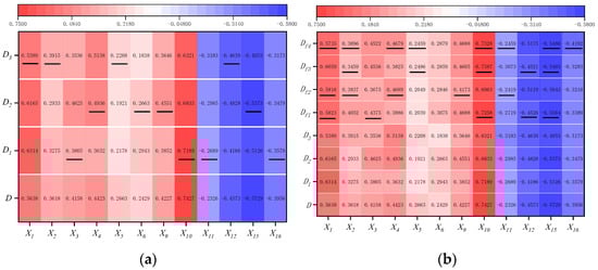
Figure 6.
PPC between input variables and matte grade: (a) PPC between input variables and matte grade in D1, D2, D3, and D; (b) PCC between input variables and matte grade in Df1, Df2, Df3, Df4, D1, D2, D3, and D.
Three different combinations of activation functions are used in the GAN, resulting in different degrees of similarity between the three generated data and the real data. In Figure 6a, the PPCs between variables X3, X10, X11, and X16 and matte grade in D1 are closer to those calculated in D. And, the PPCs between variables X4, X6, X9, and X15 and matte grade in D2 are closer to those calculated in D. Similarly, the PPCs between variables X1, X2, X5, and X12 and matte grade in D3 are closer to those calculated in D.
In summary, the data generated by the GANs with different activation functions can represent some variables similarly to real data. But, none of the GANs with a single activation function fail to globally characterize the positive features and negative features. The generated data and real data have local similarity. Therefore, a data fusion criterion based on RMSE and R2 was further designed to fuse the data generated by the three GANs.
In order to determine the optimum data fusion strategy, four different data fusion experiments were designed, as shown in Table 5.
Table 5.
Different data fusion experiments.
Firstly, the generated data D1 and D2 under Nash equilibrium were obtained using RGAN and LRGAN, respectively. And then, the weights of D1 and D2 were calculated using Equations (10) and (11), respectively. The results are shown in Table 6. Finally, the weighted fusion of D1 and D2 based on RMS and R2 was performed using Equation (12) to obtain the fused data Df1.
Table 6.
Generated data weight calculation results 1.
Similarly, we calculated the correlation weights of the other fusion experiments. And, Df2, Df3, and Df4 were obtained, as shown in Table 7, Table 8 and Table 9.
Table 7.
Generated data weight calculation results 2.
Table 8.
Generated data weight calculation results 3.
Table 9.
Generated data weight calculation results 4.
The PCC between the input variables and matte grade in Df1, Df2, Df3, and Df4 were calculated. And, the variables closest to real data were found in the fused data, as shown in Figure 6b.
From Figure 6b, it can be seen that there are eight process variables X1, X2, X4, X5, X10, X11, X15, and X16 in Df4 with a matte grade. The PPCs are closer to those calculated in D. Df4 is the most similar to the real data. It is indirectly illustrated that the Df4 obtained from the data fusion criterion based on RMSE and R2 can adequately characterize the positive and negative features of copper melting data, thus improving the quality of the generated data.
4.3.2. Visualization of Generated Data
To intuitively evaluate the quality of the data Df4, the frequency distribution histograms of the 12 input variables and matte grade in the real data D and the generated data Df4 are completed, respectively, as shown in Figure 7.
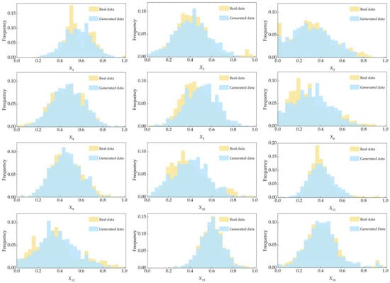
Figure 7.
The frequency distribution histogram of the real data D and the generated data Df4.
Secondly, the normal distribution curves of the 12 input variables and matte grade in the real data D and the generated data Df4 are shown in Figure 8 and Figure 9b; it can be seen that there is a large overlap between the generated data and real data, which further illustrates that the generated data are reliable.
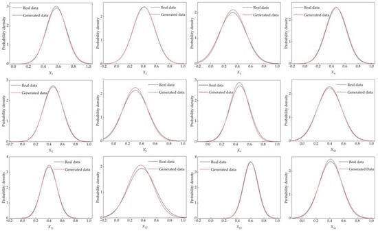
Figure 8.
The normal distribution curve of the generated data Df4 and the real data D.
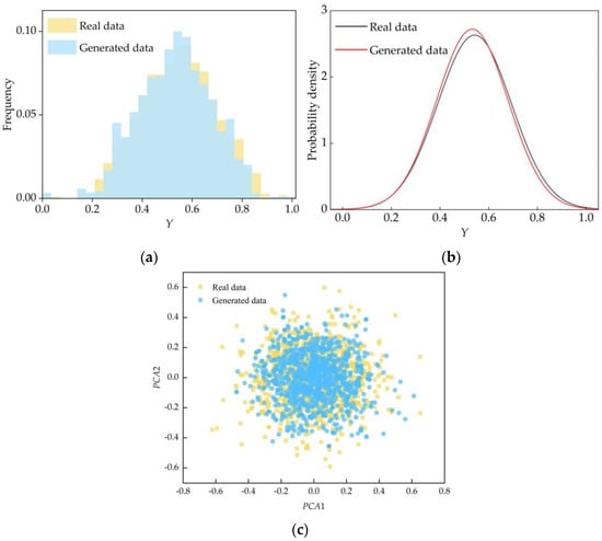
Figure 9.
Comparison of generated data with real data: (a) frequency distribution histogram; (b) normal distribution curve; (c) PCA dimension reduction.
Finally, from the perspective of inter-variable relationships, the 12 input variables of the generated data Df4 and the real data D were reduced to two dimensions using principal component analysis (PCA) dimensionality reduction, as shown in Figure 9c. We can see that the generated data and real data have a large overlap in the middle portion of the graphs, which indicates that the generated data are basically in agreement with real data and further illustrates the accuracy and reliability of the generated data after fusion.
4.4. Prediction Results and Analysis of Matte Grade
4.4.1. Evaluation Index of Matte Grade Prediction Model
There are four model evaluation metrics used in this paper, which are mean absolute error (MAE), mean absolute percentage error (MAPE), RMSE, and R2. MAE is the average value of the prediction error, which reflects how well the problem of offsetting errors can be avoided. RMSE measures the deviation of the predicted value from the true value. MAPE is a relative measure, which reflects the deviation of the predicted value relative to the true value. And, R2 represents the extent to which the independent variable explains the dependent variable. The smaller MAE, RMSE, and MAPE, the smaller the deviation of the predicted value from the true value. The smaller deviation, the better the model prediction effect. The closer the value of R2 is to 1, the stronger the model fitting ability and the better the model prediction effect []. The formulas for the four evaluation indicators are shown in Equations (28)–(31).
where denotes the predicted value; y denotes the true value; is the mean of the real data; and n denotes the number of samples in the test set.
4.4.2. Visualization of Matte Grade Prediction Results
In order to reflect the advantage of RF in matte grade prediction, the RF, Linear Regression (LR), Support Vector Regression (SVR), Long and Short-Term Memory Network (LSTM), and Backpropagation Neural Network (BP) models were used for matte grade prediction. In order to more accurately evaluate the generalization and stability of the model, we used a five-fold cross validation method. The performances of each model on the test set are shown in Table 10, and the results indicate that the RF model has the best prediction performance, with an RMSE of 0.8498, MAE of 0.3691, MAPE of 0.6251, and R2 of 0.7628.
Table 10.
Comparison of matte grade prediction experimental results from different models.
In order to verify the effectiveness of the method proposed in this paper, the ablation experiments conducted in this paper and their results are shown in Table 11.
Table 11.
Comparison of results of ablation experiments.
Firstly, the RF and MRMR_RF methods were used to predict the matte grade, and the experimental results are shown in Figure 10a. In MRMR_RF model, RMSE is reduced by 6.67%, MAE is reduced by 6.61%, MAPE is reduced by 7.17%, and R2 is increased by 2.43%. This shows that the MRMR-based variable screening method can find important input variables and improve the prediction accuracy of the matte grade.
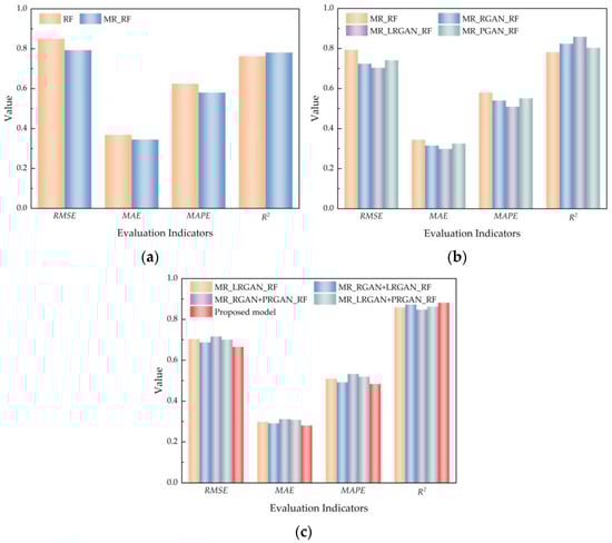
Figure 10.
Comparison of ablation experiments: (a) variable selection experiment comparison; (b) data enhancement experiment comparison; (c) data fusion experiment comparison.
Secondly, MRMR_RGAN_ RF, MRMR_LRGAN_RF, and MRMR_PRGAN_RF were used to predict the grade of matte. The experimental results are shown in Figure 10b. Compared to the MRMR_RF model, the RMSE is reduced by at least 6.52%, the MAE is reduced by at least 5.63%, the MAPE is reduced by at least 5.00%, and the R2 is increased by at least 2.82%, indicating that the GAN-based data enhancement method can effectively improve the prediction accuracy of the matte grade.
Finally, MRMR_RGAN + LRGAN_RF, MRMR_RGAN + PRGAN_RF, MRMR_ LRGAN + PRGAN_RF, and MRMR_EGAN_RF were used to predict the matte grade. The experimental results are shown in Figure 10c. The proposed method has the highest prediction accuracy. Compared to single GAN data enhancement models, RMSE is reduced by at least 5.47%, MAE is reduced by at least 6.03%, MAPE is reduced by at least 5.10%, and R2 is increased by at least 2.68%, which proves that data fusion can further improve the prediction accuracy of the matte grade.
Furthermore, to visualize the distribution of the prediction errors of different models for matte grade, the difference between the predicted value and the real value of the matte grade was calculated, and the error distribution curve is presented in Figure 11a. Compared with other models, the prediction error of MRMR_EGAN_RF is the smallest. The real value and predicted value of the matte grade obtained by different models are taken as horizontal and vertical coordinates, respectively, and the scatter plot is drawn, as shown in Figure 11b. Among them, the blue regression line represents the prediction results of the MRMR_EGAN_RF model. Compared with the prediction results of matte grade obtained by other methods, the scatter plot of the proposed method has a large number of points distributed near y = x, and the predicted matte grade is between 53% and 62%. The prediction accuracy of the proposed method is the highest, which proves the effectiveness of the proposed method.
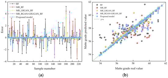
Figure 11.
Visualization of the prediction results: (a) map of the distribution of the prediction error of matte grade; (b) scatter plot of the distribution of the actual and predicted values of matte grade.
4.5. Interpretability Analysis
To improve the interpretability of the prediction results, the SHAP theory is used to explain and analyze the prediction results of the MRMR-EGAN-RF model [].
By using the SHAP method, the contribution of different parameters to predicting the matte grade can be explored. Figure 12a shows the SHAP values for each parameter. The positive/negative SHAP value of each parameter indicates that the parameter promotes/suppresses the predicted matte value, and the color of the dots represents the size of the specific value. For a certain parameter, the wider the horizontal coverage range, the greater the impact of the parameter on the prediction results, so the parameters are more important. The average of the absolute SHAP values of all data were calculated for each parameter for the parameter importance ranking, as shown in Figure 12b.
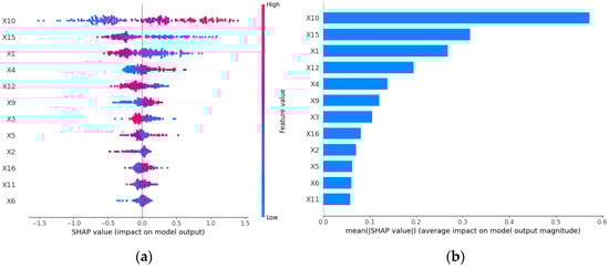
Figure 12.
Parameters importance. (a) SHAP values of different features for different samples. (b) Feature importance ranking by SHAP.
The interpretation of matte grade prediction for two different test groups of samples is shown in Figure 13. The values in the graph intuitively represent the specific impact of each variable on the predicted matte grade. The results indicate that the oxygen concentration and the Cu content in the copper concentrate have a significant positive impact on the predicted matte grade. When the oxygen enrichment concentration and copper content in the copper concentrate are high, it will push the predicted value of the model towards the direction of increasing the base value because a higher oxygen enrichment concentration can improve the oxidation reaction rate. The Isa furnace can often maintain a higher temperature, thereby improving the fluidity of the slag and more effectively removing impurities from the melt, thereby improving the matte grade. The above analysis is consistent with the experimental results, indicating that SHAP theory can improve the interpretability of the prediction models, thereby guiding users to optimize the copper smelting process.
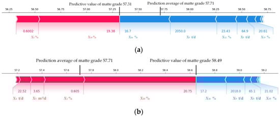
Figure 13.
Contribution of each feature to the local samples. (a) Test sample 1. (b) Test sample 2.
5. Conclusions
Aiming to address the problem of the low prediction accuracy of a matte grade prediction model due to the scarcity of samples in the copper melting process, this paper proposes the MRMR_EGAN_RF model for matte grade prediction. The MRMR algorithm is introduced to select variables that have a great influence on the matte grade. And, we use GANs with different activation functions to enhance the data and fuse different generated data based on RMSE and R2 to improve the quality of the generated data. A matte grade prediction model based on RF is proposed. The actual data collected from the industrial site are utilized to carry out the application validation and comparative analysis. The experimental results show that the proposed method can obtain high-quality generated data, and the prediction accuracy is better than other models. The R2 is improved by at least 2.68%, and other indicators such as RMSE, MAE and MAPE are significantly improved.
In future studies, we will use sensitivity analysis techniques to determine the parameters that have a significant impact on matte grade. Through a weighted analysis of the parameters, a more effective decision-making in the copper smelting process will be completed. At the same time, in order to effectively capture the key information of input variables on matte grade at different time points, we will further explore the time correlation between input variables and matte grade in the copper smelting process, construct a time attention mechanism, and improve the accuracy of matte grade prediction.
Author Contributions
Conceptualization, H.M., Z.L. and B.S.; methodology, H.M., Z.L., B.Y. and J.M.; software, H.M., B.S., B.Y. and J.M.; validation, H.M., Z.L., B.S. and B.Y.; formal analysis, H.M and Z.L.; investigation, Z.L., B.Y. and B.S.; resources, H.M., B.S., B.Y. and J.M.; data curation, Z.L., B.S. and B.Y.; writing—original draft preparation, H.M. and Z.L.; writing—review and editing, H.M. and Z.L.; visualization, H.M. and Z.L.; supervision, B.S. and B.Y.; project administration, Z.L. and B.S.; funding acquisition, J.M. and B.Y. All authors have read and agreed to the published version of the manuscript.
Funding
This research was supported by Yunnan Major Scientific and Technological Projects (grant NO. 202202AG050002).
Data Availability Statement
Since the data is part of the ongoing research, the data set provided in this paper is not easy to obtain.
Acknowledgments
Thanks to Chuxiong Dianzhong Nonferrous Metals Co., Ltd. for providing assistance and resources, and thanks to my classmate Zhang Junjia for his valuable suggestions, making it possible for us to complete this research.
Conflicts of Interest
Author Bo Shu and Bin Yu was employed by the company Chuxiong Dianzhong Nonferrous Metals Co., Ltd. The remaining authors declare that the research was conducted in the absence of any commercial or financial relationships that could be construed as a potential conflict of interest.
References
- Zhao, L.; Zhu, D.F.; Liu, D.F.; Wang, H.T.; Xiong, Z.M.; Jiang, L. Prediction and Optimization of Matte Grade in ISA Furnace Based on GA-BP Neural Network. Appl. Sci. 2023, 13, 4246. [Google Scholar] [CrossRef]
- Wang, G.B.; Yang, Y.B.; Zhou, S.W.; Li, B.; Wei, Y.G.; Wang, H. Data Analysis and Prediction Model for Copper Matte Smelting Process. Metall. Mater. Trans. 2024, 55, 2552–2567. [Google Scholar] [CrossRef]
- Yu, S.Y.; Wang, J.L.; Peng, X.B. Prediction model of craft parameters based on neural network during the process of copper flash smelting. J. Cent. South Univ. (Sci. Technol.) 2007, 38, 523–527. [Google Scholar]
- Gui, W.H.; Wang, L.Y.; Yang, C.H.; Xie, Y.F.; Peng, X.B. Intelligent prediction model of matte grade in copper flash smelting process. Trans. Nonferrous Met. Soc. China 2007, 17, 1075–1081. [Google Scholar] [CrossRef]
- Yang, C.H.; Xie, M.; Gui, W.H.; Peng, X.B. A Prediction Model for Matte Grade in Copper Flash Smelting Process. Inf. Control. 2008, 37, 28–33. [Google Scholar]
- Peng, X.B.; Gui, W.H.; Li, Y.G.; Wang, L.Y.; Chen, Y. Copper flash smelting parameter soft sensor based on dynamic T-S recurrent fuzzy neural network. Chin. J. Sci. Instrum. 2008, 29, 2029–2033. [Google Scholar]
- Liu, J.H.; Gui, W.H.; Xie, Y.F.; Wang, Y.L.; Jiang, Z.H. Key process indicators predicting for copper flash smelting process based on projection pursuit regression. Chin. J. Nonferrous Met. 2012, 22, 3255–3260. [Google Scholar]
- Zhang, X.L.; Yao, S.W.; Hu, J.H.; Dong, R.S.; Wang, H. Adaptive Soft Measurement of Process Parameters of ISA Furnace during Copper Melting Based on Generalized Maximum Entropy Regression. J. Kunming Univ. Sci. Technol. (Nat. Sci. Ed.) 2012, 37, 19–25+67. [Google Scholar]
- He, M.Q.; Yu, G.; Yang, C.; Han, L. Dynamic soft sensor modeling of matte grade in copper oxygen-rich side blow bath smelting process. Measurement 2023, 223, 113792. [Google Scholar]
- Ge, Y.Z.; Xu, X.; Yang, S.R.; Zhou, Q.; Shen, F.R. Survey on Sequence Data Augmentation. J. Front. Comput. Sci. Technol. 2021, 15, 1207–1219. [Google Scholar]
- Kegel, L.; Hahmann, M.; Lehner, W. Feature-based comparison and generation of time series. In Proceedings of the 30th International Conference on Scientific and Statistical Database Management, Bozen-Bolzano, Italy, 9–11 July 2018; pp. 1–12. [Google Scholar]
- Goodfellow, I.; Pouget-Abadie, J.; Mirza, M.; Xu, B.; Warde-Farley, D.; Qzair, S.; Courville, A.; Bengio, Y. Generative adversarial networks. Commun. ACM 2020, 63, 139–144. [Google Scholar] [CrossRef]
- Ma, Z.R.; Wang, J.J.; Feng, Y.S.; Wang, R.K.; Zhao, Z.H.; Chen, H.W. Hydrogen yield prediction for supercritical water gasification based on generative adversarial network data augmentation. Appl. Energy 2023, 49, 120814. [Google Scholar] [CrossRef]
- Hao, X.C.; Dang, H.; Zhang, Y.X.; Liu, L.; Huang, G.L.; Zhang, Y.F.; Liu, J.B. SSP-WGAN-Based Data Enhancement and Prediction Method for Cement Clinker f-CaO. IEEE Sens. J. 2022, 22, 22741–22753. [Google Scholar] [CrossRef]
- Chen, Z.S.; Hou, K.R.; Zhu, M.Y.; Xu, Y.; Zhu, Q.X. A virtual sample generation approach based on a modified conditional GAN and centroidal Voronoi tessellation sampling to cope with small sample size problems: Application to soft sensing for chemical process. Appl. Soft Comput. J. 2021, 21, 107070. [Google Scholar] [CrossRef]
- Wu, Y.J.; Li, Z.X.; Wang, Y.Z.; Guo, W.H.; Lu, B.H. Study on the Process Window in Wire Arc Additive Manufacturing of a High Relative Density Aluminum Alloy. Metals 2024, 14, 330. [Google Scholar] [CrossRef]
- Chen, Z.S.; Zhu, M.Y.; He, Y.L.; Xu, Y.; Zhu, Q.X. Quantile regression CGAN based virtual samples generation and its applications to process modeling. CIESC J. 2021, 72, 1529–1538. [Google Scholar]
- Yao, Z.J.; Zhao, C.H.; Li, Y.L.; Fu, C.; Qiao, H.L. Customized generative adversarial data imputation model for industrial soft sensing. Control. Decis. 2021, 36, 2929–2936. [Google Scholar]
- Gao, F.; Shao, X.Y. Prediction of annual electricity consumption based on feature selection and iJaya-SVR. Control. Decis. 2024, 39, 1039–1047. [Google Scholar]
- Zhang, S.F.; Li, T.M.; Hu, C.H.; Du, D.B.; Si, X.S. Missing data generation method and its application in remaining useful life prediction based on deep convolutional generative adversarial network. Acta Aeronaut. Astronaut. Sin. 2022, 43, 441–455. [Google Scholar]
- Boto, F.; Murua, M.; Gutierrez, T.; Casado, S.; Carrillo, A. Data Driven Performance Prediction in Steel Making. Metals 2022, 12, 172. [Google Scholar] [CrossRef]
- Huang, Q.Y.; Yan, N.; Zhong, X.J. Wind Power Ramping Events Prediction Based On Generative Adversarial Network. Acta Energiae Solaris Sin. 2023, 44, 226–231. [Google Scholar] [CrossRef]
- Hao, X.C.; Liu, L.; Huang, G.L.; Zhang, Y.X.; Zhang, Y.F.; Dang, H. R-WGAN-based multitimescale enhancement method for predicting f-CaO cement clinker. IEEE Trans. Instrum. Meas. 2021, 71, 1–10. [Google Scholar] [CrossRef]
- Ma, J.Y.; Liang, P.W.; Yu, W.; Chen, C.; Guo, X.J.; Wu, J.; Jiang, J.J. Infrared and visible image fusion via detail preserving adversarial learning. Inf. Fusion 2020, 54, 85–98. [Google Scholar] [CrossRef]
- Chang, J.T.; Qiao, Z.X.; Kong, X.G.; Yang, S.K.; Luo, C.W. Novel Product Duration Prediction Method of Complicated Product Based on Multi-Dimensional Nonlinear Feature Reconstruction and Fusion. J. Mech. Eng. 2023, 59, 294–308. [Google Scholar]
- Zhao, H.L.; Lu, T.T.; Yin, P.; Mu, L.Z.; Liu, F.Q. An Experimental and Simulated Study on Gas-Liquid Flow and Mixing Behavior in an ISASMELT Furnace. Metals 2019, 9, 565. [Google Scholar] [CrossRef]
- Yan, L.Q.; Wang, Z.L. Multi-step predictive soft sensor modeling based on STA-BiLSTM-LightGBM combined model. CIESC J. 2023, 74, 3407–3418. [Google Scholar]
- Liu, C.H.; Li, W.L.; Jiao, J.; Wang, J.X.; Zhang, J.N. An Interpretable Cloud Platform Task Termination State Prediction Method. J. Comput. Res. Dev. 2024, 61, 716–727. [Google Scholar]
Disclaimer/Publisher’s Note: The statements, opinions and data contained in all publications are solely those of the individual author(s) and contributor(s) and not of MDPI and/or the editor(s). MDPI and/or the editor(s) disclaim responsibility for any injury to people or property resulting from any ideas, methods, instructions or products referred to in the content. |
© 2024 by the authors. Licensee MDPI, Basel, Switzerland. This article is an open access article distributed under the terms and conditions of the Creative Commons Attribution (CC BY) license (https://creativecommons.org/licenses/by/4.0/).