The Key Process Factors in Prestressed Laser Peen Forming and the Design of Parameters Through an Artificial Neural Network

Abstract

This research investigated the influences of some key factors in the prestressed laser peen forming (PLPF) process, namely, the plate thickness, the coverage ratio, and the prestress, on the deformation of 2024-T351 rectangular plates through experiments and numerical simulations. In the experiments, laser parameters, such as the laser energy and spot size, were kept unchanged, and prestress was applied through a piece of self-developed, four-point-bending equipment. The curvature radius of the samples was measured through a digital radius gauge. A corresponding finite element analysis (FEA) model of PLPF was also established to simulate the full procedure of the PLPF, including prebending, laser shock peening, and spring back. Based on the PLPF experimental results, an artificial neural network (ANN) was trained to help to design the process parameters, including the coverage ratio and the amount of prebending, according to the plate thickness and the target curvature radius. By adding a penalty term to the loss function, the amount of prebending (AOP) can be reduced as much as possible. The validation of the ANN was confirmed by three other PLPF experiments.

1. Introduction

In the manufacturing of complex thin-walled structures, such as integrated panels, in the aerospace industry, shot peen forming (SPF) is a widely used processing method. SPF is a kind of plastic-forming technology, which uses a hard projectile flow to shoot the external surface of the target metal plate. In this process, plastic deformation and compressive residual stress are induced, and the metal plate will bend because the stress gradient in the direction of the plate thickness is not zero. When the deformation is not sufficient, the technique of prestress is often employed to reinforce the forming ability of SPF. The process of SPF assisted by prestress is called prestressed shot peen forming (PSPF). Prestress is generally applied using a certain set of bending equipment. Thus, the process of applying prestress is also called prebending.

Moreover, with the evolution of laser technology, laser shock peening (LSP) is introduced to the plastic-forming process, which is then known as laser peen forming (LPF). The principle of LSP is the interaction between the laser pulse and material, as shown in Figure 1. When a high-energy, short-duration laser pulse irradiates the absorbent layer, the irradiated material will quickly vaporize and become plasma within a few nanoseconds. In this process, the plasma will expand rapidly and form a laser-supported detonation wave. This detonation wave will impact the test plate and leave plastic deformation and residual stress on the surface of and inside the material and is able to cause the target to deform. Similar to PSPF, prestress could also theoretically assist the LPF process, which is then called prestressed LPF (PLPF).

There have been a substantial number of studies on SPF and PSPF in recent decades. Miao et al. discussed the effects of SPF parameters, including prestress, on the bending moment and residual stress of aluminum alloy 2024 plate samples through experiments, in 2010, confirming that prestress is able to help to increase the arc height of deformed plates and reduce the tendency for spherical surfaces to form in PSPF plates [1]. In 2011, they focused on the finite element analysis (FEA) of PSPF. The prestress was directly applied to the plate model as the initial stress [2]. Wang et al. researched the deformation behavior of 8-to-12 mm thick aluminum alloy 7150 plates in PSPF [3]. An experimental study by Wang et al., in 2016, introduced an example of the application of PSPF in the formation of rebar-stiffened integral panels [4]. Xiao et al. discussed the influences of prestress and the coverage ratio on plate deformation in PSPF through experiments and numerical simulations, in which a relation among the crater diameter, shot velocity, and the amount of prestress was established [5]. In 2018, Faucheux et al. reported their research on a method for simulating PSPF with eigenstrains, the validation of which was confirmed through XRD residual stress measurements and optical deformed shape measurements [6]. Faucheux and colleagues researched the effects of prestress and material anisotropy on plate deformation, in 2022. In their research, a series of PSPF experiments were carried out on 4.9 mm long 2024-T3 plates [7].

The research method of LPF is similar to that of SPF. Studies on LPF began in the 1970s. Based on the pioneering research of Anderholm et al., O’Keefe et al., Fabbro et al., and others [8,9,10,11,12,13], studies on laser shock peening (LSP) have been improved, especially in the past two decades, because of the advancements in laser and robot technologies. In 2005, Liu et al. established a method to design an LPF process to form doubly curved shapes through FEA, the validation of which was verified by LPF experiments [14]. Zhou et al. proposed an innovative PLPF process, which uses the thermal effect of lasers to achieve the application of prestress, in 2007 [15]. Hua et al. performed some research on the deformation of aluminum plates in LPF [16]. In brief, in LPF, a metal plate can bend to form a convex or concave surface at different plate thicknesses, fundamentally reflecting the residual stress. However, in 2015, Sticchi et al. focused mainly on the influences of the spot size and material properties on the residual stress [17]. Fang et al. discussed the improvement of the forming ability of LPF by elastic preloading [18]. Hu et al. presented a study about the effect of the prestress on LPF deformation using the eigenstrain-based model [19]. In 2018, Hatamleh et al. reported their research on damping profiles in numerical simulations of LPF [20]. Li et al. also conducted some numerical and experimental research on PLPF, in which the influences of the coverage ratio, spot size, and amount of prebending were discussed [21]. Moreover, Nguyen et al. presented the difference between water-confined and air-confined LPF shockwaves [22]. In 2020, Wang et al. discussed grain refinement in LSP at the microscale according to dislocation dynamics [23]. Xiong et al. also discussed the effects of the confinement and coating on LSP at the microscale [24]. In 2024, Jiang et al. proposed a topology-optimization-based process planning method for LPF to determine peening patterns with multiple process conditions, demonstrating superior results compared to those obtained using a consistent process condition [25]. Abhishek et al. investigated the use of array-type laser shock peening (ALSP) with round spots to reduce residual stress hole generation, finding that the proper parameter selection can minimize this effect, especially for small-impact-radius configurations [26].

In production, the parameters provided by the design department mainly include the thickness and target curvature radius. The production department needs to design the spot array and amount of prebending according to these parameters. This study used an artificial neural network (ANN) to assist in this process. An ANN is a computational model inspired by the human brain’s structure and function. It consists of layers of interconnected nodes or neurons that process information through weighted connections. ANNs are capable of learning from data, making them powerful tools for pattern recognition, classification, and prediction tasks. The applications of ANNs in LPF are still limited. In 2021, Wu et al. predicted laser-shock-induced residual stress through an ANN [27]. In 2023, Sala et al. introduced an ANN using genetic algorithm to predict the deformed shape of LPF [28]. Zhao et al. also published their research about residual stress prediction in LSP [29]. They built a physics-informed machine-learning model and achieved a fairly high accuracy degree.

This research on PLPF is based on previous studies and focuses on the influence of the prestress on the bending deformation of LSP-treated rectangular 2024-T351 plate samples. Moreover, other important process factors in LPF, including the plate thickness and coverage ratio, are also discussed. Based on the experimental data (100 groups in total), a simple but effective ANN is built to design the process parameters. The results and findings in this research can be used to guide the industrial application of PLPF.

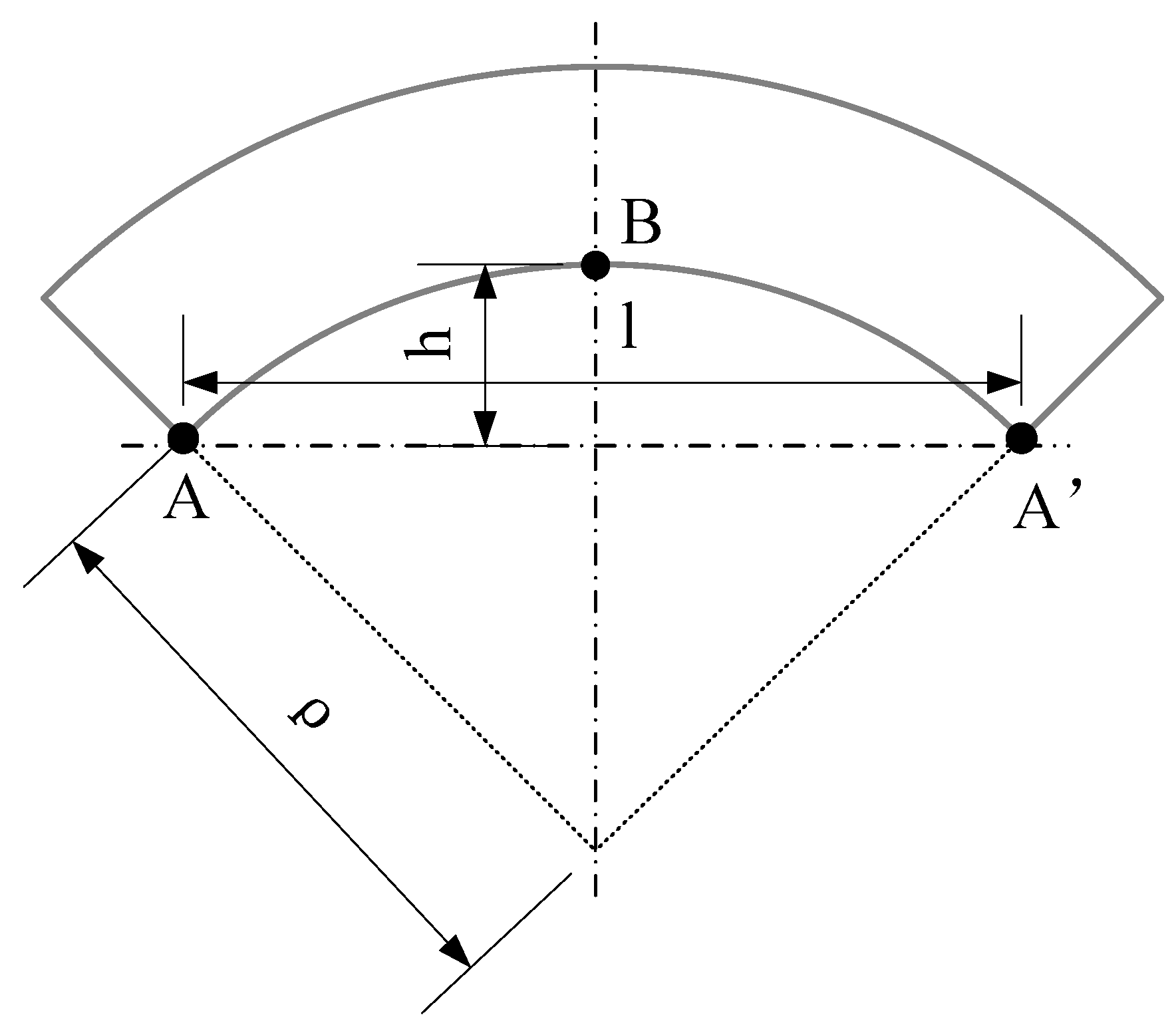
2. Mechanics of Prebending

Generally, prestress is applied to a metal sheet workpiece through bending. Consequently, the process of prestressing could also be called prebending. In this research, a piece of four-point-bending equipment was developed and adopted, the schematic of which is shown in Figure 2. The part of the plate between the two movable holders is theoretically pure bending (Figure 3). Thus, in the elastic range, the stress in the thickness direction is linearly distributed, and on the top surface, the tensile stress reaches its maximum. The amount of prebending (AOP) is defined as the ratio of the magnitude of the tensile stress on the top surface (${\sigma }_t$) (also the maximum stress in the section) to the tensile yield stress (${\sigma }_s$). Obviously, the AOP should be no larger than 100% to ensure that prebending is an elastic process.

$$AOP={\displaystyle \frac{{\sigma }_t}{ {\sigma }_s}} \times 100\%.$$

(1)

In the experiment, the AOP was characterized by the curvature radius of the test plate after prebending. In elastic mechanics, the bending curvature at the mid-surface ($k$) is linear to the bending moment ($M$) as follows:

$$k={\displaystyle \frac{M}{EI}}.$$

(2)

where $E$ is the modulus of elasticity, and $I$ is the moment of inertia. On the other hand, because the shape of the section of the test plate is rectangular,

$${\sigma }_t={\displaystyle \frac{M}{I}}\times {\displaystyle \frac{t}{2}}.$$

(3)

where $t$ is the thickness of the plate, and $k_t$ is the curvature of the top surface. For thin plates, $k_t\approx k$. By substituting Equation (2) into Equation (3), Equation (4) is obtained as follows:

$${\sigma }_t={\displaystyle \frac{1}{2}}{k}_{t}Et.$$

(4)

The radius of curvature (${\rho }_t$) is

$${\rho }_t={\displaystyle \frac{1}{k_t}}={\displaystyle \frac{Et}{2{\sigma }_t}}.$$

(5)

Thus, the AOP can also be defined via the curvature radius as follows:

$$AOP={\displaystyle \frac{{\rho }_s}{{\rho }_t}}\times 100\%.$$

(6)

In this research, the material of the test plates was aluminum alloy 2024-T351, which has been widely used in the aerospace industry. After uniaxial tensile tests, the yield strength (${\sigma }_s$) of the material was 369 MPa. Additionally, the ${\rho }_s$ values of plates of different thicknesses can be calculated.

Moreover, the coverage ratio (CR) in LPF ($\eta$) is defined in Equation (7) and is shown in Figure 4, where $r_0$ is the spot radius, and $d$ is the spot distance. The distances of the laser spot in the longitudinal and transverse directions are equal in this research.

$$\eta ={\displaystyle \frac{\pi r_0^2}{d^2}}\times 100\%.$$

(7)

Through prebending, the material at the top surface could be considered to be in a uniaxial tensile stress state. This makes it easier for plastic deformation to occur in the prebending direction. Theoretically, prebending induces mechanical anisotropy in the material.

3. Experimental Research on LPF

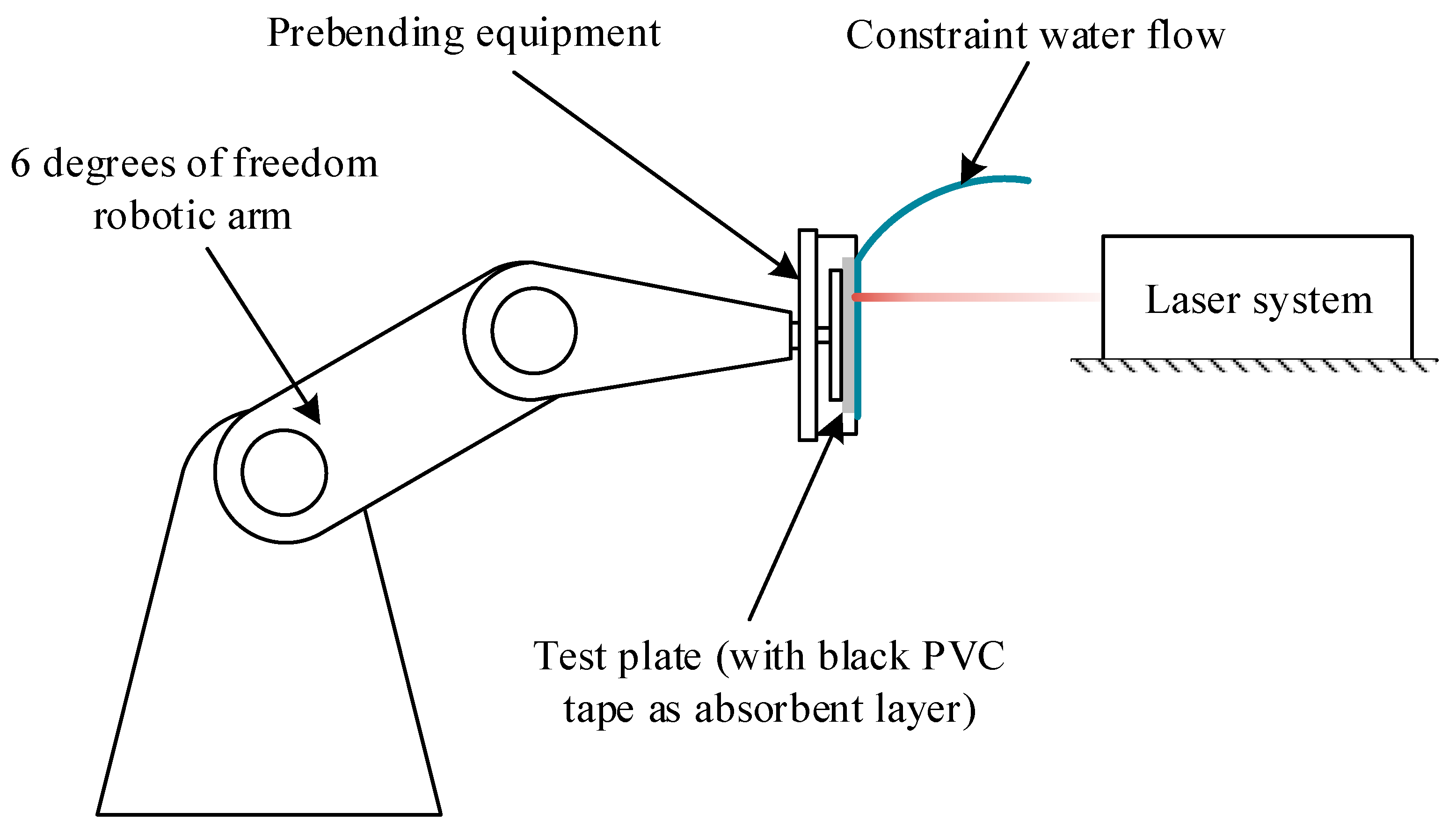
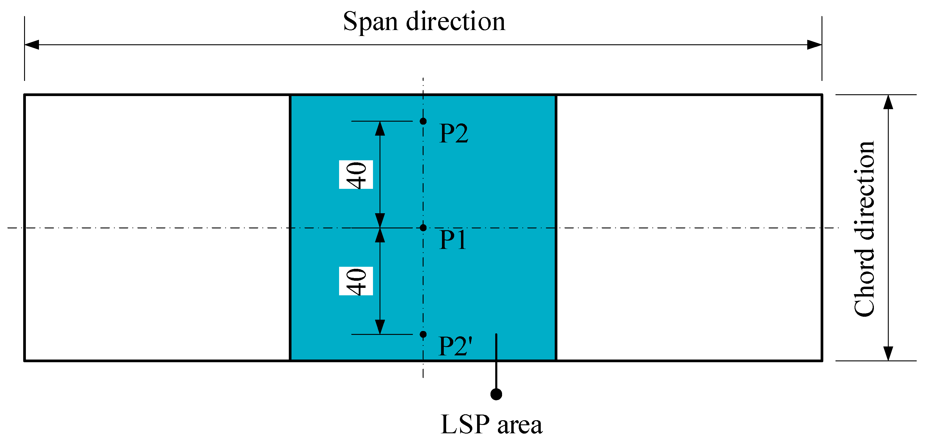
3.1. Experimental Design

This research aimed to determine the effect of prestressing on LPF. Thus, the main variable was the amount of prebending, AOP. In addition, the influences of the plate thickness and coverage ratio were also discussed. The other variables involved in this research were the plate thickness ($t$) and the coverage ratio ($\eta$). The laser parameters, such as the laser energy, laser pulse width, and spot size, were kept constant. The laser parameters are listed in

Table 1. Laser parameters.

$\mathbf{Laser} \mathbf{Energy}, {\mathit{E}}_{\mathit{l}\mathit{a}\mathit{s}}$	$\mathbf{Full} \mathbf{Width} \mathbf{at} \mathbf{Half} \mathbf{Maximum} \left(\mathbf{FWHM}\right) \mathbf{of} \mathbf{Laser} \mathbf{Pulse}, \mathit{\tau }$	$\mathbf{Spot} \mathbf{Radius}, {\mathit{r}}_0$	$\mathbf{Laser} \mathbf{Wavelength}, \mathit{\lambda }$
75 J	20 ns	5 mm	1063 nm

. The laser power density was limited to a lower level to ensure that the absorbent material within the LSP-treated area was not burnt out and that the surface of the sample was not ablated by the laser pulse. If there is no requirement for surface quality, a stronger laser pulse can be applied, and the forming ability will be stronger. The main independent variables are listed in

Table 2. Main independent variables in the LPF experiment.

$\mathbf{Plate} \mathbf{Thickness}, \mathit{t}$ (mm)	$\mathbf{Spot} \mathbf{Distance}, \mathit{d}$ (mm)	$\mathbf{Coverage} \mathbf{Ratio}, \mathit{\eta }$	AOP
4; 6; 8; 10; 12	7.0; 10.0; 11.2; 12.5; 15.0	160.3%; 78.5%; 62.1%; 50.3%; 34.9%	0; 50%; 75%; 100%

. In Table 2, the coverage ratio is dependent on the spot distance; thus, there are actually only three main variables: the plate thickness, spot distance, and AOP. A group of complete experiments based on the variable-control method was conducted, for a total of 100 experiments.

The experiments were carried out on 300 × 100 mm² 2024-T351 rectangular plates, as shown in Figure 5. The specimens were cut using wire electrical discharge machining from a 55 mm thick rolled 2024-T351 plate and then milled to the target size. In order to avoid the problem of the anisotropy of the material, the orientation of all the specimens was consistent. The span direction of the specimens was perpendicular to the rolling direction. The 100 × 100 mm² area in the middle was the LSP area as well as the pure bending section.

The prebending equipment was self-designed and made of 40# carbon structural steel to ensure its stiffness. The supplier of this equipment is the process equipment institute of AVIC Xi’an Aircraft Industry Co., Ltd. (Xi’an, China). It can be used in both LPF and SPF. Figure 6 shows a photograph of the equipment with the test plate being prestressed. In the photo in Figure 7, the radius of curvature of the 4 mm plate for an experiment with an AOP of 50% was measured. A digital radius gauge was adopted to measure the radii of curvature of the prestressed and LSP-treated test plates. The digital radius gauge contains a digital micrometer indicator and a series of rigid bridges with a standard span.

The experiments were conducted at AECC Beijing Institute of Aeronautical Materials, Beijing, China. The LSP device, as shown in Figure 8, was equipped with a Nd:YAG solid laser system, which could output five circular flat-top laser pulses per second. The laser system was fixed, and the prebending equipment, together with the test piece, was held and moved by a robotic arm. The absorbent layer in LSP was black PVC tape, which is used to absorb the laser energy and generate a plasma explosion, and the constraint layer was a water flow film to confine the plasma explosion and intensify the shock pressure.

3.2. Experimental Results and Discussion

The dependent variable measured in this experiment was the curvature radius along the span direction of the test plate, namely, the prebending direction. Figure 9 shows the positions of the three measurement points, P1, P2, and P2′. P1 was located at the center of the LSP area; P2 and P2′ were symmetrical about the spanwise axis, and the distance between them was 80 mm. They were located at the back surface of the test plate because the front surface was filled with LSP craters. The span of the bridge on the radius gauge was 60 mm. The average of the three measured values was the final measured value.

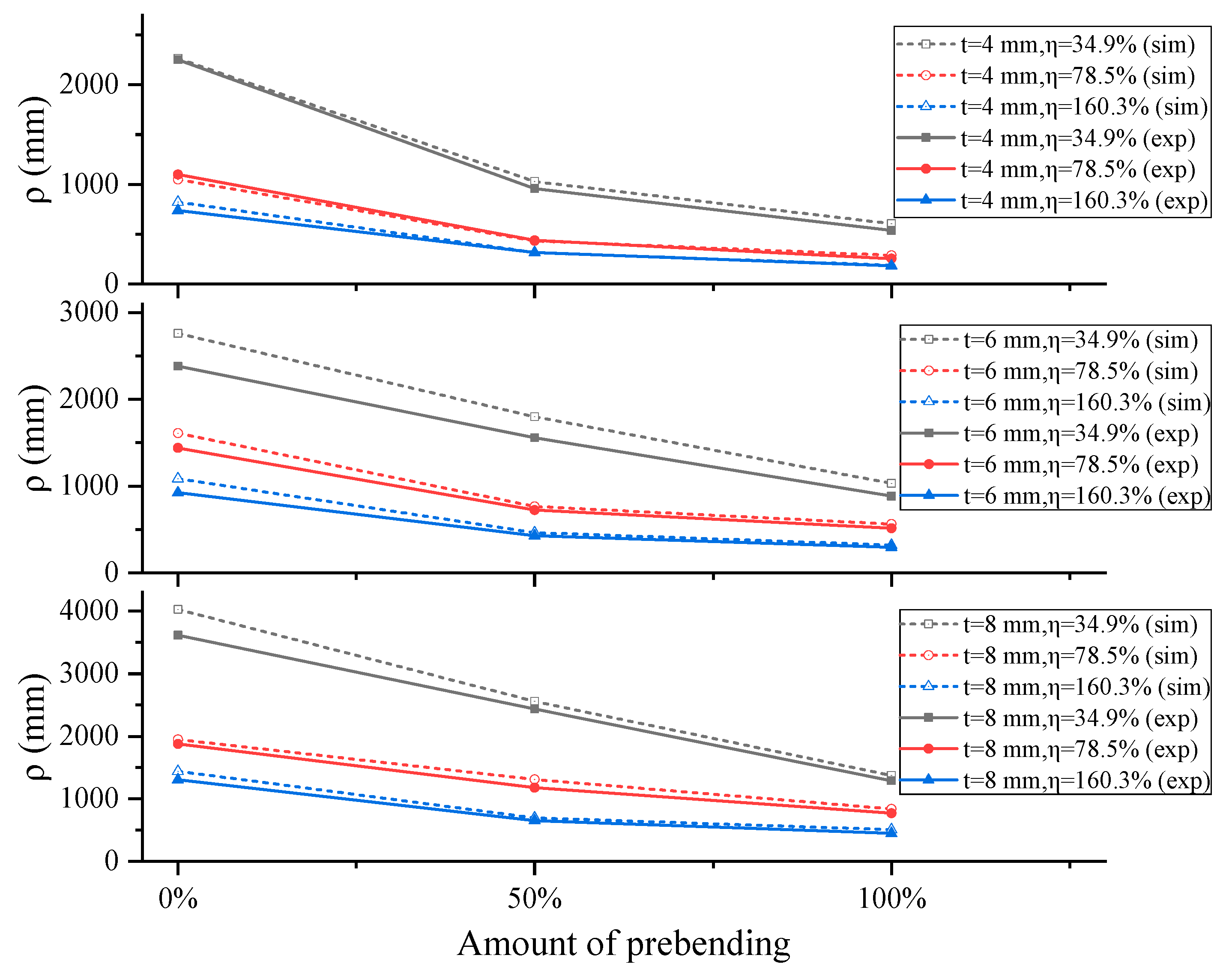
3.2.1. Influence of Prestress

Generally, the process of prestressing was proven to be effective through the results of the experiments. Figure 10 shows the change in the curvature radius with respect to the AOP. With increasing AOP, the curvature radius of the deformed plate markedly decreased. Under most conditions, the radius when the AOP = 100% is 30–40% of that when the AOP = 0. The effect of the prestress was more significant when the AOP changed from 0 to 50% than when it changed from 50% to 100%.

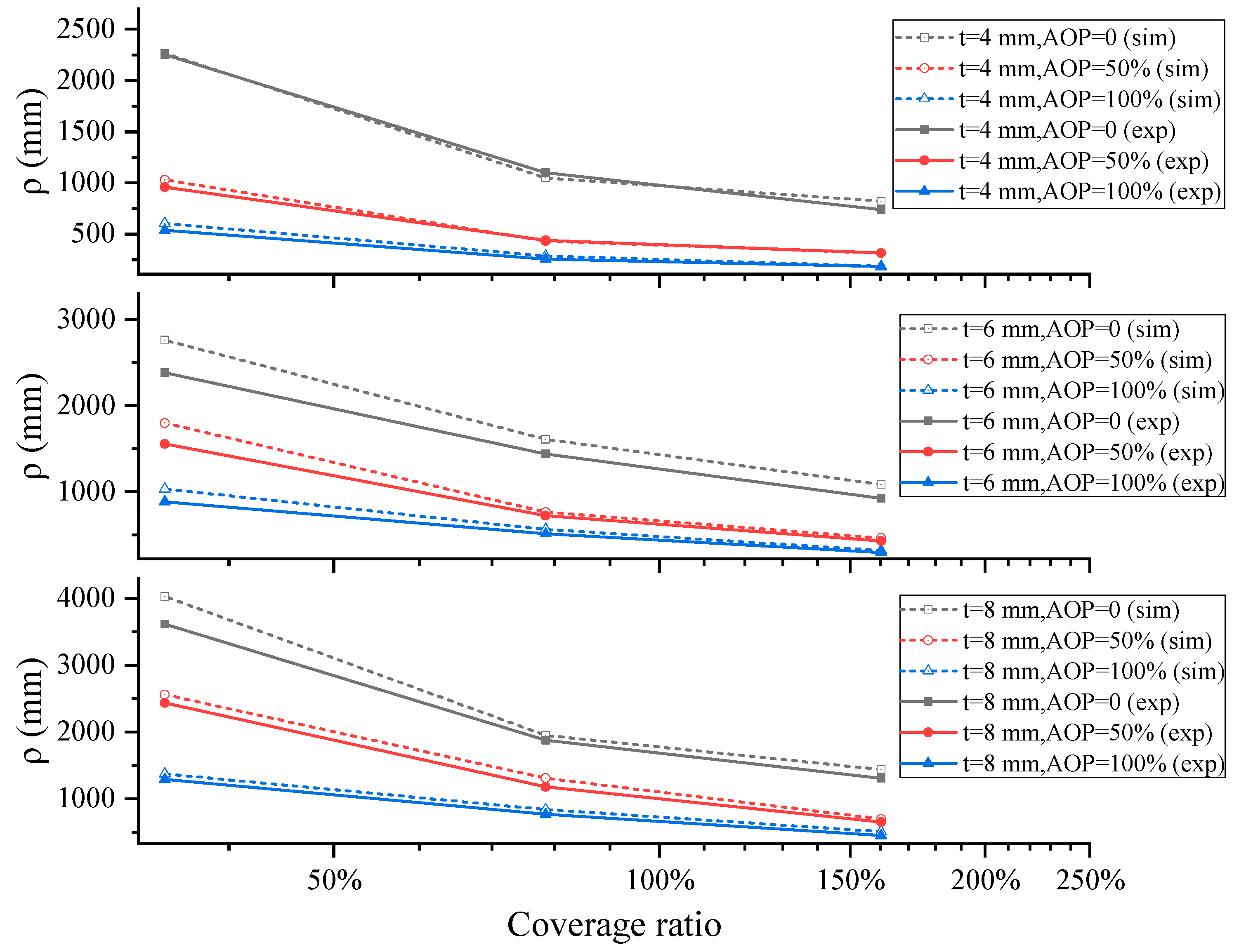
3.2.2. Influence of the Coverage Ratio

The influence of the coverage ratio is shown in Figure 11. With increasing coverage ratio, the curvature radius apparently decreased. In Figure 11, the AOP = 50–100% lines were close to each other and were separated from the AOP = 0 line. It could also be concluded that with increasing AOP, the effect decreased. When the other parameters were kept constant, the radius when the AOP = 100% was 30–40% of the radius when the AOP = 0. At the same time, the number of abnormal points that do not conform to the general trend is highest in Figure 11, and their distribution is relatively random. This indicates that the CR may be a variable that is difficult to control, and its influence on deformation exhibits a certain degree of uncertainty.

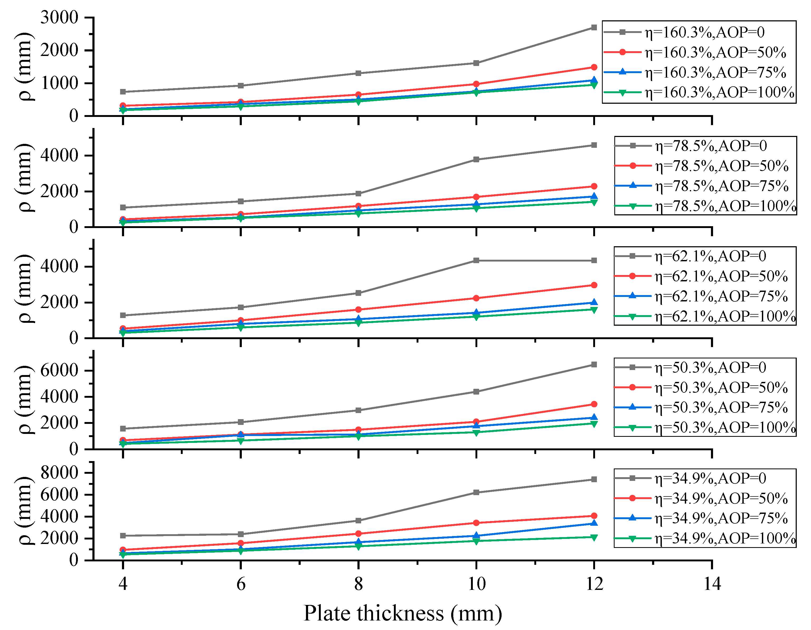
3.2.3. Influence of Plate Thickness

Figure 12 shows that thicker plates are harder to deform, while prebending can significantly increase the forming ability of the LPF. When the AOP increased from 0 to 100%, the curvature radius of the 12 mm thick plate decreased about 67.5% on average. However, for thinner plates, prebending appears to be more effective. For a 4 mm thick plate, the curvature radius at AOP = 1 decreases to approximately 24.5% of that at AOP = 0.

3.2.4. Discussion

Notably, there were several abnormal data points. These points did not follow the overall rule of the change. This phenomenon was mostly caused by the residual stress of the sample processing, including plate rolling and machining. Moreover, the AOP was difficult to control during the actual experiment. In the LSP process, as the residual stress is induced and the plate gradually deforms, the moment of the prebending changes. Consequently, the AOP actually changes during the laser shock process, which may introduce uncertainty to the eventual deformation.

4. Finite Element Analysis

Although the LSP process uses laser processing, because the laser irradiation time is very short, only at the nanosecond level, heat conduction cannot be completed in such a short duration. In addition, because of the absorbent layer used in LSP, the laser will not be directly irradiated to the surface of the metal workpiece, and the water flow constraint layer also plays a role in heat dissipation. Therefore, the effect of the temperature is ignored in this FEA model, and LSP is considered to be a mechanical process.

4.1. Numerical Model of Laser Shock Pressure

This section introduces the variation in the distribution and magnitude of the laser shock pressure ($P$) with time. Assuming that the spatial and temporal amplitude functions are $p_s(r,\theta )$ (in the cylindrical coordinate system) and $p_t\left(t\right)$ and that the maximum laser shock pressure is $P_0$, $P$ can be described by the following equation:

$$P=P_0·p_s\left(r,\theta \right)·p_t\left(t\right).$$

(8)

4.1.1. Determination of P₀

The widely used formula for calculating $P_0$ was first proposed by Peyre et al. in 1996 [12], as follows:

$$P_0\left(GPa\right)=0.01\sqrt{{\displaystyle \frac{\alpha }{2\alpha +3}}}\sqrt{Z\left(g·{\mathrm{c}\mathrm{m}}^{-2}·s^{-1}\right)}\sqrt{I_0\left(\mathrm{G}\mathrm{W}·{\mathrm{c}\mathrm{m}}^{-2}\right)}.$$

(9)

In Equation (9), $\alpha =0.1–0.2$ is the efficiency of the laser energy transferring to the shock pressure, $Z$ is the reduced shock impedance, and $I_0={\displaystyle \frac{E_{las}}{\pi {r_0}^2·\tau }}$ is the laser power density. For simplification, $P_0$ is often given as Equation (10) [30].

$$P_0\left(GPa\right)=K\sqrt{I_0\left(\mathrm{G}\mathrm{W}·{\mathrm{c}\mathrm{m}}^{-2}\right)}.$$

(10)

For different confinements, absorbents, laser wavelengths, and target materials, the value of $K$ is also variable. Hfaiedh et al. reported that K = 1.65 when $I_0=3~8 \mathrm{G}\mathrm{W}·{\mathrm{c}\mathrm{m}}^{-2}$, and the confinement is water for aluminum 2050-T8 plates [30], which is similar to the current situation. Consequently, it was decided that K = 1.65 in this research.

4.1.2. Spatial Distribution of the Shock Pressure (p_s)

On the other hand, the output laser beam is a flat-top beam, which is transferred from a Gaussian beam generated by a Nd:YAG solid laser through optical elements. This procedure follows the law of the conservation of energy, indicating that the laser intensity on a certain section, $I(z,r)$, is as follows:

$$I\left(z,r\right)=I_{max}{\int }_0^{2\pi }d\theta {\int }_0^{\omega \left(z\right)}{e}^{-{\displaystyle \frac{2r^2}{{\omega \left(z\right)}^2}}}dr={A\pi {\omega \left(z\right)}^2·I}_{max}.$$

(11)

where $I_{max}$ is the maximum laser intensity, $r$ is the distance of a point on the section from the optical axis, $z$ is the location of the section on the optical axis, and $\omega \left(z\right)$ is the radius of the section. $A$ is the average amplitude of the flat-top beam. By solving Equation (11), $A\approx 0.787$; thus,

$$p_s\left(r,\theta \right)=\sqrt{A}\approx 0.887.$$

(12)

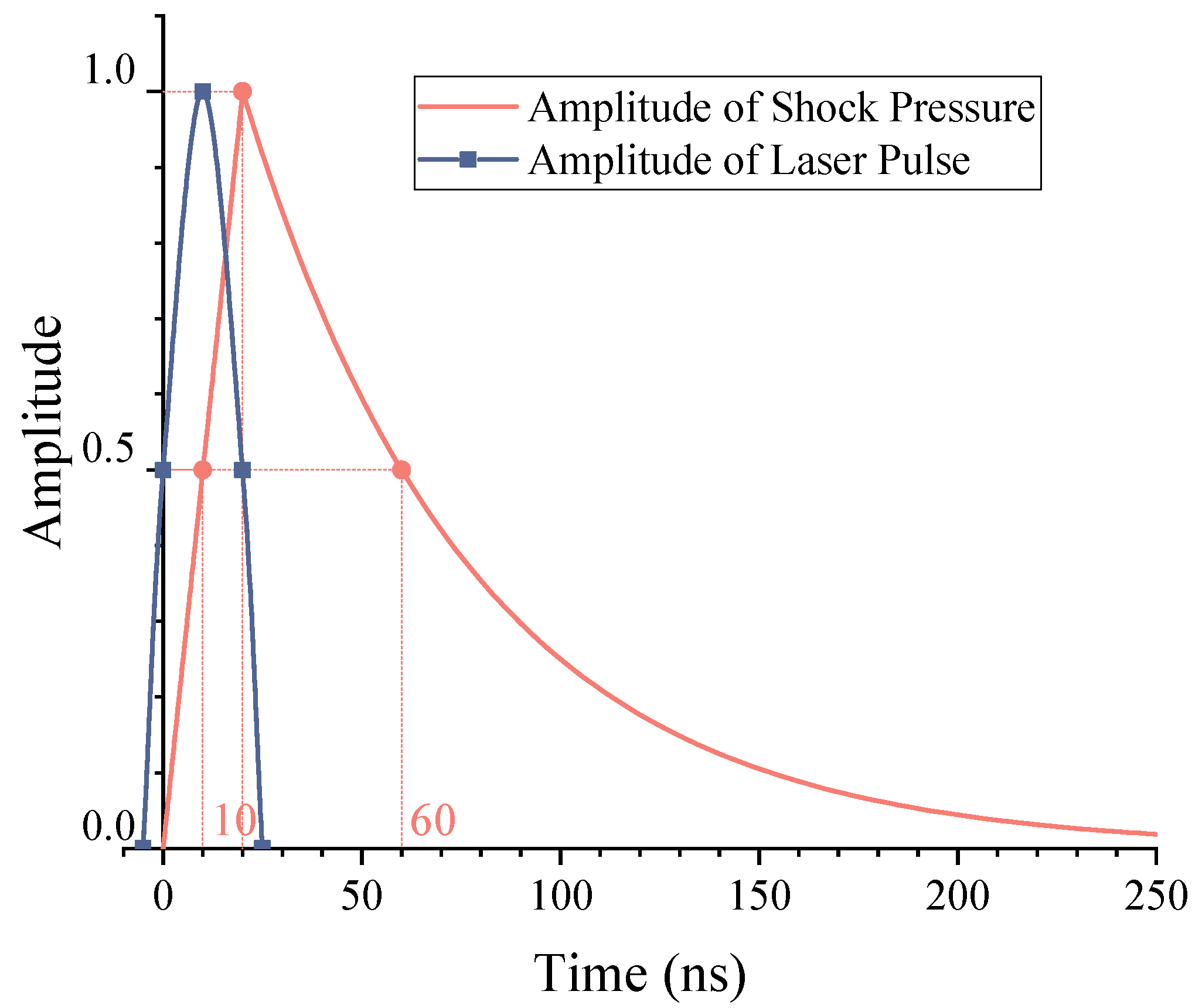
4.1.3. Temporal Distribution of the Shock Pressure (p_t)

Many studies have been conducted to determine the variation in laser shock pressure with time. Generally, the curve of $p_t\left(t\right)$ has a rapid ascending part and a slow descending part. In this research, to describe this rule, a piecewise function (Equation (13)) was adopted, in which $C_1$, $C_2$, and $C_3$ are undetermined coefficients ($C_1,C_2,C_3>0$), composed of a linear ascending part when $0<t\le \tau$ and an exponential descending part when $t>\tau$.

$$p_t\left(t\right)=\left\{\begin{array}{c}{\displaystyle \frac{1}{C_1}}{\tau }_{las} \left(0<t\le \tau \right)\\ \exp \left[-C_2\left(t-C_3\right)\right] \left(t>\tau \right)\end{array}\right..$$

(13)

Hfaiedh considered that the FWHM of the shock pressure is 2–3 times that of a laser pulse [30]; thus, the FWHM of the shock pressure was set at $50 \mathrm{n}\mathrm{s}$, which is 2.5 times that of $\tau$. Consequently, the following set of equations can be obtained:

$$\left\{\begin{array}{c}{p}_t\left(\tau \right)={\displaystyle \frac{1}{C_1}}\tau =1\\ p_t\left(\tau \right)=\exp \left[-C_2\left(\tau -C_3\right)\right]=1\\ p_t\left(3\tau \right)=\exp \left[-C_2\left(3\tau -C_3\right)\right]=0.5\end{array}\right..$$

(14)

By solving Equation (14), $p_t\left(t\right)$ can be determined (i.e., Equation (15)). Figure 13 presents the amplitude curves of the laser pulse and shock pressure. It should be noted that the curve of the laser pulse is given qualitatively and only to perform the time order of the laser pulse and pressure pulse.

$$p_t\left(t\right)=\left\{\begin{array}{c}{\displaystyle \frac{1}{\tau }}t \left(0<t\le \tau \right)\\ \exp \left(-{\displaystyle \frac{\ln \left(2\right)}{2\tau }}\left(t-\tau \right)\right) \left(t>\tau \right)\end{array}\right..$$

(15)

4.2. Material Properties of 2024-T351

The strain rate could reach ${10}^{-6} {\mathrm{s}}^{-1}$ in LSP. Consequently, the Johnson–Cook plasticity model was classically adopted to describe the dynamic behaviors of metallic materials in the LSP procedure. The flow stress of the J-C model ($\overline{\sigma }$) is given by Equation (16), in which $A$ is the initial yield stress, $B$ is the work-hardening modulus, ${\overline{\epsilon }}^{pl}$ is the equivalent plastic strain, $n$ is the work-hardening coefficient, $C$ is the strain rate sensitivity, ${\dot{\overline{\epsilon }}}^{pl}$ is the equivalent plastic strain rate, and ${\dot{\epsilon }}_0$ is the reference strain rate. For 2024-T351, the J-C model parameters are listed in

Table 3. Johnson–Cook parameters of 2024-T351 [31].

${\mathit{\sigma }}_{\mathit{s}}$ (MPa)	$\mathit{B}$ (MPa)	$\mathit{n}$	$\mathit{C}$	${\dot{\mathit{\epsilon }}}_0$ (s−1)
369	684	0.73	0.0083	1

. Other necessary material properties include the elastic modulus at $72.6 \mathrm{G}\mathrm{P}\mathrm{a}$, Poisson’s ratio at 0.33, and the density at $7700 \mathrm{k}\mathrm{g}/{\mathrm{m}}^3$.

$$\overline{\sigma }=\left[{\sigma }_s+B{\left({\overline{\epsilon }}^{pl}\right)}^n\right]\left[1+Cln\left({\displaystyle \frac{{\dot{\overline{\epsilon }}}^{pl}}{{\dot{\epsilon }}_0}}\right)\right].$$

(16)

4.3. FEA Model of PLPF

FEA was carried out in Abaqus/CAE 2022. As shown in Figure 14, the 1/4 FEA model included two holders, which were analytical rigid bodies, and the test plate, a 3D deformable body. The symmetry planes were XY and YZ. The meshes in the LSP area were refined to 0.4 mm in the X and Z directions and 0.2 mm in the Y direction. For the 4 mm plate, a total of 447,500 cubic elements were created.

FEA contains three main steps:

(1)

Prebending: The movable holder moves upward, contacts the test plate, and finally pushes the plate to meet the target AOP, as shown in Figure 14(a2,b). In this step, the static, implicit solver is invoked;

(2)

LSP treatment: The states of strain and stress and the deformation condition of the prebent plate are transferred to the model of this step through the predefined field function. Laser shock pressure is applied to the surface of the LSP area through the Abaqus Fortran subscript VDLOAD. This procedure uses the dynamic, explicit solver;

(3)

Spring back: The shape, stress, and strain of the plate after the LSP treatment are also transmitted through the predefined field. With all the constraints of the holders removed, a static analysis is used to calculate the final condition of the test plate.

The LSP parameters used in the FEA were the same as those used in the experiments. However, not all the experiments were simulated. In

Table 4. Main independent variables in the LPF simulation.

$\mathbf{Plate} \mathbf{Thickness}, \mathit{t}$ (mm)	$\mathbf{Spot} \mathbf{Distance}, \mathit{d}$ (mm)	$\mathbf{Coverage} \mathbf{Ratio}, \mathit{\eta }$	AOP
4; 6; 8	7.0; 10.0; 15.0	160.3%; 78.5%; 34.9%	0; 50%; 100%

, the parameters used in the simulation are presented. In total, 27 groups of simulations were conducted.

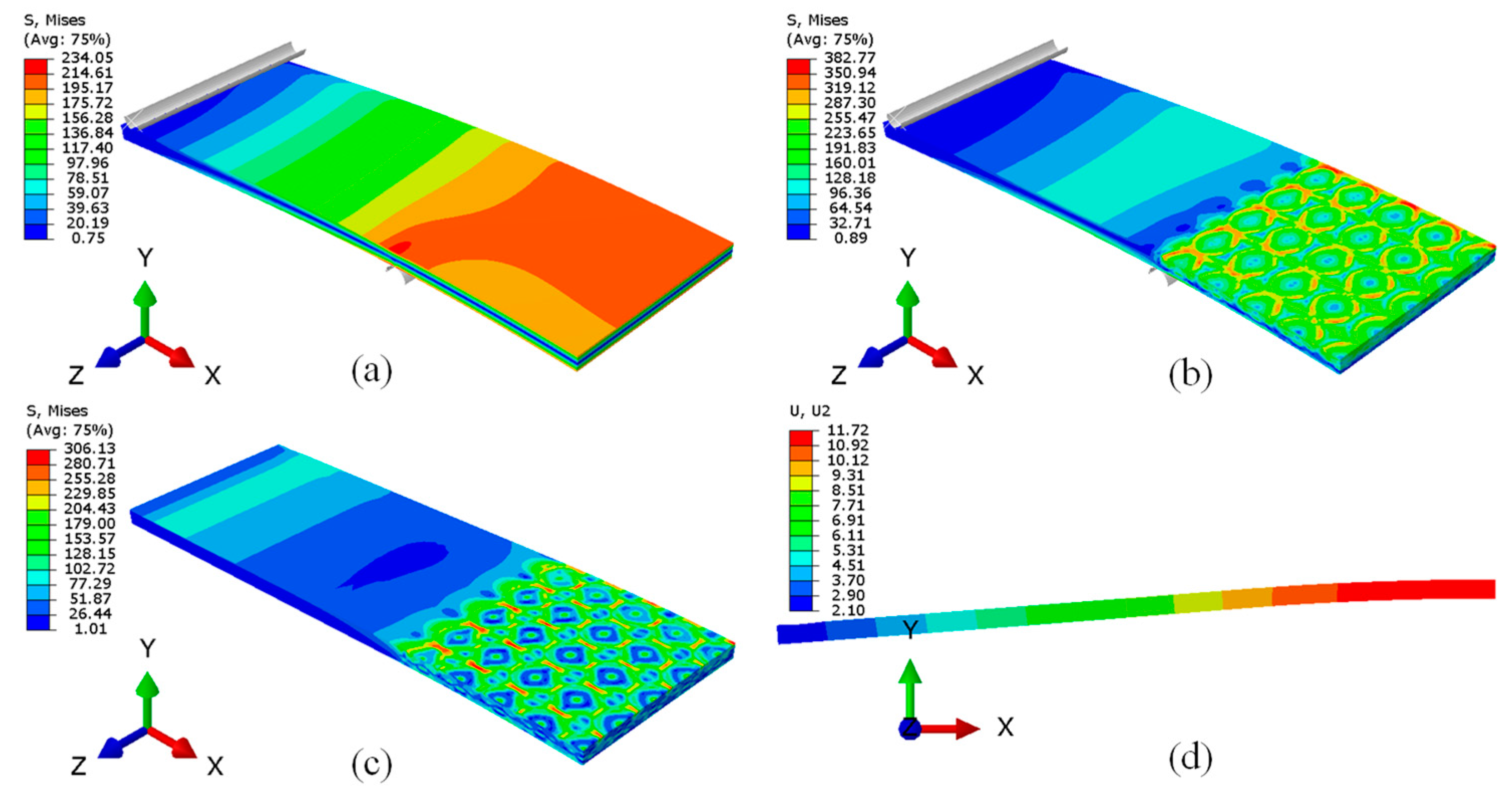
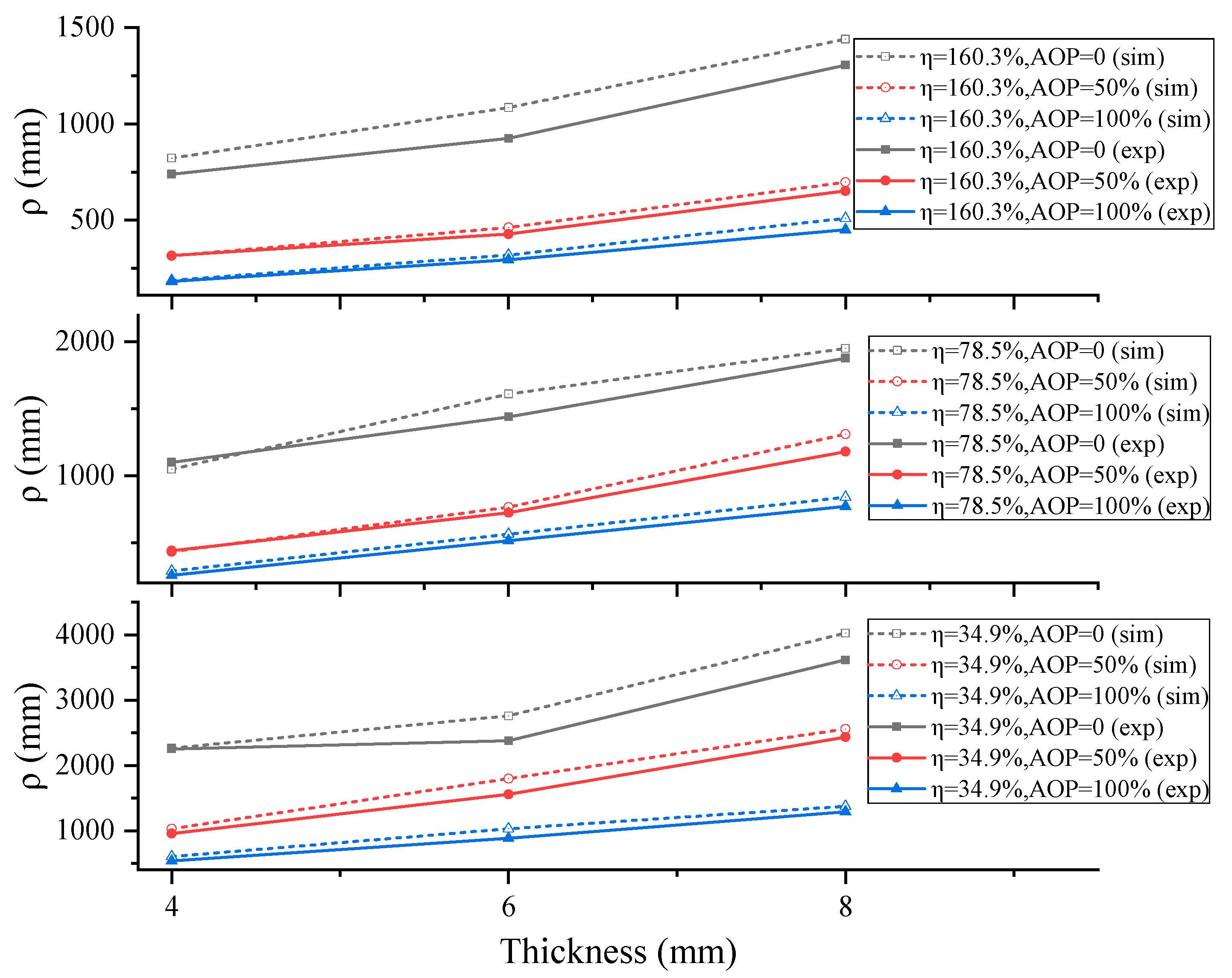
4.4. Simulation Results and Discussion

In Figure 15, an example of the stress contours after the completion of each step and the final displacement contour are displayed. The plate thickness is 4 mm, the coverage ratio is 78.5%, and the AOP is $50\%$. In Figure 15a, the maximum stress appears at the contact position of the plate and holder. The stress on the top surface is about 195 MPa, which is half of ${\sigma }_s$. This agrees with the AOP. From Figure 15b,c, as the constraint of the prebending equipment on the plate is removed, the plate rebounds, and the stress value decreases. The final deformation of the plate is shown in Figure 15d. This research mainly focusses on the deformation condition of the plates after the treatment with PLPF, more specifically, the curvature radius. As for the digital radius gauge, the calculation of the simulated plate curvature radius was also based on the arc height, as shown in Figure 16, where $l$ is the deformed distance between $A$ and $A^{\prime }$, the two borders of the LSP area; the arc height is $h$, and $\rho$ is the curvature radius. According to the Pythagorean theorem, Equation (17) can be obtained. Because $h^2$ can be considered as an infinitely small quantity compared with ${\rho }^2$ and is ignored, the solution of Equation (17) is $\rho ={\displaystyle \frac{l^2}{8h}}$. Consequently, the values of ${\displaystyle \frac{l}{2}}$ and $h$ were extracted from the output database (.ODB) file, and the curvature radii of a total of 27 groups of simulations were calculated.

$${\left({\displaystyle \frac{1}{2}}l\right)}^2+{\left(\rho -h\right)}^2={\rho }^2.$$

(17)

According to the FEA results, the curvature radius values were calculated and drawn in Figure 17, Figure 18 and Figure 19. The change rule of $\rho$ is generally the same as that of the experimental results. With increasing AOP and coverage ratio and decreasing plate thickness, the curvature radius tends to decrease, which is favorable for deformation. However, the simulation results tend to be larger than the experimental results. When the AOP is small (AOP = 0), the simulation results are not reliable. To further analyze the relative error of the simulation results, the average errors of every single independent variable were calculated and are listed in

Table 5. Average relative errors of simulation results.

$\mathbf{Plate} \mathbf{Thickness}, \mathit{t}$ (mm)	Relative Error	AOP	Relative Error	$\mathbf{Coverage} \mathbf{Ratio}, \mathit{\eta }$	Relative Error
4	5.90%	0	9.67%	0.35	10.16%
6	12.08%	0.5	6.79%	0.79	7.71%
8	8.55%	1	10.07%	1.6	8.65%

. The average error of all the data is 8.84%. It can be found that for smaller AOPs and higher coverage ratios, the simulation error tends to be larger. It is speculated that the reason is related to the clamping of the specimen by the prebending equipment. For the case of the AOP = 0, there is a certain force between the movable holder and the specimen when the specimen is clamped. Otherwise, the specimen may fall off from the holder during the LSP process. Consequently, the actual AOP is slightly greater than zero. Without the influence of gravity in the FEA, there will be no such problem, so AOP = 0 in the simulation.

5. PLPF Parameter Design Assisted by an ANN

During the production of thin-walled components via LPF, there can be various combinations of process parameters to achieve the desired curvature radius. Generally, to attain the same curvature radius, a higher CR corresponds to a smaller AOP. A larger AOP typically requires more complex processing equipment, whereas a higher CR implies longer processing times. Moreover, while keeping the laser parameters constant, to achieve the same curvature radius, reducing the AOP will necessarily increase the CR. From the perspective of reducing production costs, compared to extending the processing time, increasing the complexity of the prebending process is more unacceptable. Consequently, considering these characteristics of LPF, the optimization goals for process parameter design are to either maximize the CR or minimize the AOP.

Based on the data collected from the LPF experiment, an artificial neural network was constructed based on a multi-layer perceptron (MLP) and trained to calculate the CR and AOP according to the given design targets (curvature radius and plate thickness). Evidently, this is a regression problem with constraints. The development process was carried out using PyCharm 2022.1.2, with the help of the open-source Python machine-learning libraries PyTorch 1.12.0 and Scikit-learn 1.1.2 and the open-source Python development library Numpy.

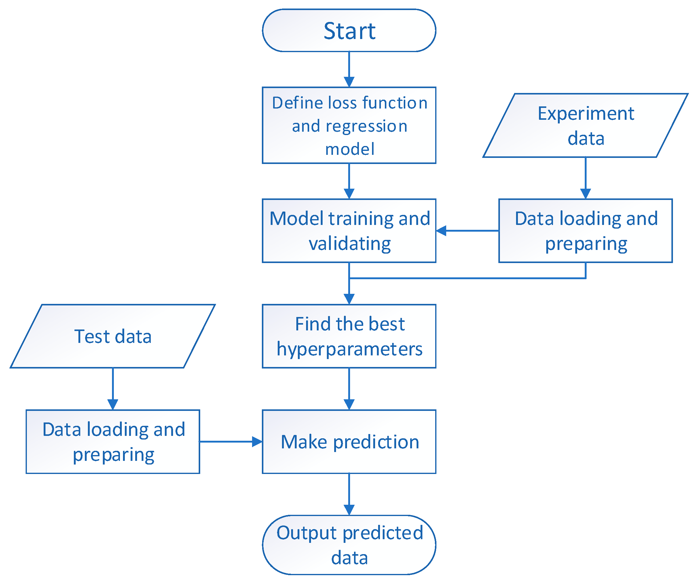
5.1. Code Structure Overview

The flowchart of the program is shown in Figure 20. This code implements a regression task on a specific dataset by defining a custom loss function, constructing a neural network model, training the model, evaluating the model’s performance, and, ultimately, outputting the optimal hyperparameters along with their corresponding predictions. By running multiple experiments, the code enables users to identify the best-performing models within the given hyperparameter ranges.

The code consists of several key components:

(1)

Defining a loss function and a regression model: This defines a custom loss function that includes mean-square-error (MSE) terms, a regularization term, and an AOP penalty term, tailored to meet the needs of optimizing the LSP process. The expression of the loss function ($L$) is shown in Equation (18), in which ${MSE}_{CR}$ and ${MSE}_{AOP}$ are the MSEs of the coverage ratio and AOP. $R$ is the regularization term, and $\lambda$ is the weight of $R$. Herein, the LASSO regularization method was adopted, $w_{AOP}$ is the AOP penalty term, and $\alpha$ is the weight of the AOP.

$$L={MSE}_{CR}+{MSE}_{AOP}+\lambda \cdot R+\alpha \cdot w_{AOP}.$$

(18)

In addition, a fully connected ANN model, which contains two inputs, two outputs, and three hidden layers, was also defined for this regression task. Every layer was made up of 64 cells;

(2)

Data loading and preparing: This reads the original data from an Excel file, splits the data into training and testing sets, and converts them to PyTorch tensors. These data are normalized to [0, 1];

(3)

Model training and validating: This is used to train ANN models of different hyperparameters;

(4)

Finding the best hyperparameters: Within these models, the best model with the smallest total loss is chosen for prediction tasks;

(5)

Making predictions: This uses the best model to make predictions according to the test data.

The ANN program can output the predicted values of the CR and AOP, as well as the corresponding hyperparameter values and the total loss under three optimization objectives (maximizing the CR, minimizing the AOP, and minimizing the total loss).

5.2. Prediction Results and Experimental Verification

To verify the accuracy of the ANN predictions, three different combinations of target values, i.e., the plate thickness and the curvature radius, were designed, and experiments based on the predictions in these three scenarios were conducted. The target parameters, prediction results, and experimental results are shown in

Table 6. Prediction and verification experimental results.

Number	Target Parameters		Predicted Parameters		Experimental Results of Radius (mm)	Relative Error to Target Radius
	Thickness (mm)	Curvature Radius (mm)	Coverage Ratio	AOP
1-MinLoss	4	555	64.23%	68.54%	561.29	1.13%
1-MinAOP	4	555	75.12%	54.46%	584.63	5.34%
1-MaxCR	4	555	75.12%	54.46%	584.63	5.34%
2-MinLoss	5	1600	51.68%	9.04%	1621.3	1.33%
2-MinAOP	5	1600	50.21%	8.93%	1675.6	4.73%
2-MaxCR	5	1600	75.12%	54.46%	779.31	51.29%
3-MinLoss	8	1200	62.29%	72.68%	1233.2	2.77%
3-MinAOP	8	1200	75.12%	54.46%	1273.0	6.08%
3-MaxCR	8	1200	75.12%	54.46%	1273.0	6.08%

. “MinLoss” indicates that the optimization objective is to minimize the total loss, “MinAOP” means that the optimization objective is to minimize the AOP, and “MaxCR” represents that the optimization objective is to maximize the CR.

According to the error between the ANN predictions and experimental results, it was confirmed that the ANN can precisely predict the process parameters, and the prediction accuracy can reach about 99%. Minimizing the total loss can obtain the most accurate prediction results, but it often leads to a relatively larger AOP. Additionally, the outcomes of minimizing the AOP and maximizing the CR are not effective enough, and in different testing datasets, there have been numerous identical prediction results, indicating a certain degree of overfitting. This may be because of an insufficient data amount and the inefficiency of the optimization algorithm.

6. Discussion and Conclusions

In this study, a large number of PLPF experiments were designed and completed. At the same time, based on the actual prebending process and LPF process, an FEA model was designed, and its effectiveness was verified through experiments. In addition, an ANN for PLPF process parameter design was successfully designed with high prediction accuracy.

Through experimental and numerical research on PLPF, it can be concluded that prestress has a significant effect on improving deformation in the LPF process.

Compared with FEA, ANNs have advantages in both accuracy and efficiency. The calculation time of the FEA depends on factors such as the model complexity, mesh size, constraints, and computer configuration. In this study, it takes several to tens of hours to complete the FEA, and there is a large error between the calculation and experimental results. In order to obtain more reliable results, it is necessary to further increase the computational cost. Using an ANN for predictions, the model-training time only takes a few minutes, and the prediction can almost be completed in an instant.

The forming process of SPF and PSPF is not easy to control, and the forming accuracy is often low. The surface quality of the workpiece after SPF processing is also poor, but the processing efficiency is very high, and the large area can be processed in a short time. In contrast, the parameters of each laser shock of LPF are programmable, and it is easier to combine them with artificial intelligence to achieve high-precision forming, but the processing time is too long. Therefore, in the foreseeable future, LPF and PLPF will be used more as a supplement to SPF to deal with difficult-to-form structures and occasions where high forming accuracy is required. An intelligent process design of PLPF is also the goal of further research.

References

1. Miao, H.Y.; Demers, D.; Larose, S.; Perron, C.; Lévesque, M. Experimental study of shot peening and stress peen forming. J. Mater. Process Technol. 2010, 210, 2089–2102. [Google Scholar] [CrossRef]
2. Miao, H.Y.; Larose, S.; Perron, C.; Lévesque, M. Numerical simulation of the stress peen forming process and experimental validation. Adv. Eng. Softw. 2011, 42, 963–975. [Google Scholar] [CrossRef]
3. Wang, M.T.; Zeng, Y.S.; Bai, X.P.; Huang, X. Deformation Rule of 7150 Aluminum Alloy Thick Plate by Pre-Stress Shot Peen Forming. Adv. Mater. Res. 2014, 1052, 477–481. [Google Scholar] [CrossRef]
4. Wang, M.; Zeng, Y.; Huang, X.; Lv, F.; Chinesta, F.; Cueto, E.; Abisset-Chavanne, E. Research on deformation of 7050 aluminum alloy panels with stiffeners by pre-stress shot peen forming. AIP Conf. Proc. 2016, 1769, 200011. [Google Scholar] [CrossRef]
5. Xiao, X.D.; Wang, Y.J.; Zhang, W.; Wang, J.B.; Wei, S.M. Numerical research on stress peen forming with prestressed regular model. J. Mater. Process Technol. 2016, 229, 501–513. [Google Scholar] [CrossRef]
6. Faucheux, P.A.; Gosselin, F.P.; Lévesque, M. Simulating shot peen forming with eigenstrains. J. Mater. Process Technol. 2018, 254, 135–144. [Google Scholar] [CrossRef]
7. Faucheux, P.A.; Miao, H.Y.; Lévesque, M.; Gosselin, F.P. Peen forming and stress peen forming of rectangular 2024–T3 aluminium sheets: Curvatures, natural curvatures and residual stresses. Strain 2022, 58, e12405. [Google Scholar] [CrossRef]
8. Anderholm, N.C. Laser-Generated Stress Waves. Appl. Phys. Lett. 1970, 16, 113–115. [Google Scholar] [CrossRef]
9. O’Keefe, J.D.; Skeen, C.H.; York, C.M. Laser-induced deformation modes in thin metal targets. J. Appl. Phys. 1973, 44, 4622–4626. [Google Scholar] [CrossRef]
10. Fairand, B.P.; Clauer, A.H. Laser generation of high-amplitude stress waves in materials. J. Appl. Phys. 1979, 50, 1497–1502. [Google Scholar] [CrossRef]
11. Peyre, P.; Fabbro, R. Laser shock processing: A review of the physics and applications. Opt. Quant. Electron. 1995, 27, 1213–1229. [Google Scholar] [CrossRef]
12. Peyre, P.; Fabbro, R.; Merrien, P.; Lieurade, H.P. Laser shock processing of aluminium alloys. Application to high cycle fatigue behaviour. Mater. Sci. Eng. A Struct. Mater. Prop. Microstruct. Process. 1996, 210, 102–113. [Google Scholar] [CrossRef]
13. Berthe, L.; Fabbro, R.; Peyre, P.; Tollier, L.; Bartnicki, E. Shock waves from a water-confined laser-generated plasma. J. Appl. Phys. 1997, 82, 2826–2832. [Google Scholar] [CrossRef]
14. Liu, C.; Yao, Y.L. FEM-Based Process Design for Laser Forming of Doubly Curved Shapes. J. Manuf. Process 2005, 7, 109–121. [Google Scholar] [CrossRef]
15. Zhou, J.; Huang, S.; Du, J.; Chen, Y.; Sun, Y. Laser Pre-Stressed Compound Peen Forming of Plate. Chin. J. Lasers 2007, 34, 861–865. [Google Scholar]
16. Hua, D.; Yun, W.; Lan, C. Laser shock forming of aluminum sheet: Finite element analysis and experimental study. Appl. Surf. Sci. 2010, 256, 1703–1707. [Google Scholar] [CrossRef]
17. Sticchi, M.; Staron, P.; Sano, Y.; Meixer, M.; Klaus, M.; Rebelo Kornmeier, J.; Huber, N.; Kashaev, N. A parametric study of laser spot size and coverage on the laser shock peening induced residual stress in thin aluminium samples. J. Eng. 2015, 2015, 97–105. [Google Scholar] [CrossRef]
18. Fang, G.; Yao, Z.; Hu, Y. Modeling Research for Plate Pre-Loading of Laser Peening Forming. Mach. Des. Res. 2013, 29, 80–83. [Google Scholar]
19. Hu, Y.X.; Li, Z.; Yu, X.C.; Yao, Z.Q. Effect of elastic prestress on the laser peen forming of aluminum alloy 2024-T351: Experiments and eigenstrain-based modeling. J. Mater. Process Technol. 2015, 221, 214–224. [Google Scholar] [CrossRef]
20. Hatamleh, M.I.; Mahadevan, J.; Malik, A.; Qian, D. Variable Damping Profiles Using Modal Analysis for Laser Shock Peening Simulation. J. Manuf. Sci. Eng. 2018, 140, 051006. [Google Scholar] [CrossRef]
21. Li, Q.; Wan, M.; Li, W.; Huang, X.; Zeng, Y. Finite element simulation of laser shock peening forming under prestressed loading. J. Plast. Eng. 2018, 25, 21–26. [Google Scholar]
22. Nguyen, T.T.P.; Tanabe, R.; Ito, Y. Comparative study of the expansion dynamics of laser-driven plasma and shock wave in in-air and underwater ablation regimes. Opt. Laser Technol. 2018, 100, 21–26. [Google Scholar] [CrossRef]
23. Wang, C.; Wang, L.; Wang, C.; Li, K.; Wang, X. Dislocation density-based study of grain refinement induced by laser shock peening. Opt. Laser Technol. 2020, 121, 105827. [Google Scholar] [CrossRef]
24. Xiong, Q.; Shimada, T.; Kitamura, T.; Li, Z. Atomic investigation of effects of coating and confinement layer on laser shock peening. Opt. Laser Technol. 2020, 131, 106409. [Google Scholar] [CrossRef]
25. Jiang, J.; Li, Z.; Hu, Y.; Chen, S.; Song, Y.; Hu, L. Density-based topology optimization of multi-condition peening pattern for laser peen forming. Int. J. Mech. Sci. 2024, 267, 108968. [Google Scholar] [CrossRef]
26. Abhishek; Panda, S.S.; Kumar, S. Numerical Investigation of Residual Stress Field Induced by Array-Type Laser Shock Peening. JOM 2024, 76, 759–775. [Google Scholar] [CrossRef]
27. Wu, J.J.; Li, Y.H.; Zhao, J.B.; Qiao, H.C.; Lu, Y.; Sun, B.Y.; Hu, X.L.; Yang, Y.Q. Prediction of residual stress induced by laser shock processing based on artificial neural networks for FGH4095 superalloy. Mater. Lett. 2021, 286, 129269. [Google Scholar] [CrossRef]
28. Sala, S.T.; Körner, R.; Huber, N.; Kashaev, N. On the use of machine learning and genetic algorithm to predict the region processed by laser peen forming. Manuf. Lett. 2023, 38, 60–64. [Google Scholar] [CrossRef]
29. Zhao, W.; Pang, Z.C.; Wang, C.X.; He, W.F.; Liang, X.Q.; Song, J.D.; Cao, Z.Y.; Hu, S.; Lang, M.; Luo, S.H. Hybrid ANN-physical model for predicting residual stress and microhardness of metallic materials after laser shock peening. Opt. Laser Technol. 2025, 181, 111750. [Google Scholar] [CrossRef]
30. Hfaiedh, N.; Peyre, P.; Song, H.; Popa, I.; Ji, V.; Vignal, V. Finite element analysis of laser shock peening of 2050-T8 aluminum alloy. Int. J. Fatigue 2015, 70, 480–489. [Google Scholar] [CrossRef]
31. Lesuer, D. Experimental Investigations of Material Models for Ti-6A1-4V and 2024-T3; 1999. Available online: https://digital.library.unt.edu/ark:/67531/metadc623770/m2/1/high_res_d/11977.pdf (accessed on 13 April 2025).
Disclaimer/Publisher’s Note: The statements, opinions, and data contained in all the publications are solely those of the individual author(s) and contributor(s) and not of MDPI and/or the editor(s). MDPI and/or the editor(s) disclaim(s) responsibility for any injury to people or property resulting from any ideas, methods, instructions, or products referred to in the content.
Figure 1. Principle of laser shock peening.
Metals 15 00445 g001
Figure 2. Principle of four-point bending.
Metals 15 00445 g002
Figure 3. The diagrams of the force and bending moment. ( t is the plate thickness, F is the support reaction of the holder to the plate, 3 a is the length of the sample and M is the bending moment).
Metals 15 00445 g003
Figure 4. Definition sketch of the coverage ratio ( r 0 is the spot radius and d is the spot distance).
Metals 15 00445 g004
Figure 5. Test plate and laser shock peening (LSP) area ( t is the plate thickness).
Metals 15 00445 g005
Figure 6. Prebending equipment and test plate.
Metals 15 00445 g006
Figure 7. Measurement of the amount of prebending (AOP).
Metals 15 00445 g007
Figure 8. LSP device.
Metals 15 00445 g008
Figure 9. The loacations of radius measurement points P1, P2, and P2′.
Metals 15 00445 g009
Figure 10. Change in the curvature radius with the amount of prebending (AOP).
Metals 15 00445 g010
Figure 11. Change in curvature radius with the coverage ratio.
Metals 15 00445 g011
Figure 12. Change in the curvature radius with the plate thickness.
Metals 15 00445 g012
Figure 13. Amplitude curves of the laser pulse and shock pressure.
Metals 15 00445 g013
Figure 14. The FEA models of different steps of PLPF for a 4 mm test plate. (a1,a2) Prebending; (b) LSP; (c) spring back.
Metals 15 00445 g014
Figure 15. Stress contours (unit: MPa) after each step (ac) and final displacement contour (d) (unit: mm).
Metals 15 00445 g015
Figure 16. Calculation of curvature radius for simulation results ( A and A are the two borders of the LSP area, l is the deformed distance between A and A , h is the arc height, and ρ is the curvature radius).
Metals 15 00445 g016
Figure 17. Change in the curvature radius with the amount of prebending (simulations and experiments).
Metals 15 00445 g017
Figure 18. Change in the curvature radius with the coverage ratio (simulations and experiments).
Metals 15 00445 g018
Figure 19. Change in the curvature radius with the plate thickness (simulations and experiments).
Metals 15 00445 g019
Figure 20. The flowchart of the program.
Metals 15 00445 g020