Numerical Predictions of Uniform CO₂ Corrosion in Complex Fluid Domains Using Low Reynolds Number Models

Abstract

To get the knowledge of local corrosion, thinning is useful for developing targeted inspection plans for pipe components in the oil/gas industry. Aiming at this object, this work presents a computer fluid dynamics (CFD) method to predict CO₂ aqueous corrosion in complex fluid domains. The processes involved in CO₂ aqueous corrosion, including flow dynamics, mass transfer, chemical reactions, and electrochemical reactions, are modeled and simulated by a commercial CFD software of Fluent V15.0 (Version, manufacturer, city, country). Mass transfer in the straight pipe flow and jet impinging flow are simulated using three low-Reynolds-number turbulent models (Abe–Kondoh–Nagano k − ε model, Change–Hsieh–Chenk k − ε model, and k − ε shear stress transport model). The flow domains are meshed by grids with the first near-wall node at the position at y⁺ = 0.1. Comparisons between simulations and experimental data show the Abe–Kondoh–Nagano model provides the best predictions of near-wall flow and mass transfer. Thus, it is used to predict CO₂ aqueous corrosion. Corrosion rates of dissolved CO₂ in straight pipes and a jet impinging are predicted. The predicted corrosion rates are compared with experimental data and results derived from commercial software, Multicorp V5.2.105. The results show that predicted corrosion rates are reasonable. The locations of the highest corrosion rate for a jet impinging system are revealed.

1. Introduction

CO₂ gas in the presence of liquid water is a main cause of corrosion in oil/gas production and transport. Predictions of uniform CO₂ corrosion have received much attention in the past few decades. Many models, including empirical models as well as semi-empirical models [1,2,3,4,5] and mechanistic models [6,7,8,9,10,11,12,13,14], have been developed for the effects of species, water chemistry, flow, pH, water cut, temperature, and film on the overall corrosion rate.

Nesic et al. [6] presented a mechanistic model for uniform CO₂ corrosion with no protective film based on several individual electrochemical reactions, such as hydrogen ion reduction, carbolic acid reduction, water reduction, oxygen reduction, and iron dissolution. The corrosion rate can be calculated from the combination of the active current density and the diffusion-limited current density. Moreover, the latter is directly related to the mass transfer coefficient, which can be derived from the experience model of Berger and Hau [15]. Anderko [7] similarly calculated the uniform corrosion rate of selected metals in CO₂ aqueous solution. Later, Nesic and coworkers extended the model to the corrosion of high-pressure CO₂ in the presence of acetic acid (HAC) [8] and corrosion of CO₂ corrosion with hydrogen sulfide [9,10,11]. Employing these models, open source software for the prediction of uniform CO₂ corrosion was developed [12].

In the layer adjacent to a wall, electrochemical reactions on the surface consume depolarizers and produce ferrous ion. Variations in the concentrations of certain species could be reduced by homogeneous chemical reactions in the layer and molecular diffusion from the bulk to the layer. The reactions and diffusion process provide “buffers” for depolarizers and enhance the corrosion rate. Considering coupling among electrochemical reactions, chemical reactions, and diffusion processes, Nordsveen et al. [13] proposed a comprehensive mechanistic model of uniform CO₂ corrosion, covering homogenous chemical reactions in bulk and films, electrochemical reactions on a surface, species diffusion between bulk and a surface, the migration process, and the growth kinetics of films. A one-dimensional (1D) finite difference method was applied to solve the transport equations with boundary conditions derived from electrochemical reaction dynamics and convective terms substituted by turbulent diffusion terms. Additionally, Song [14] also proposed a mechanistic model of uniform CO₂ corrosion considering the effect of the O₂ and cathode protection. Electrochemical reactions, homogenous reactions, and species transport were also included in the model, but they were solved with analytical methods. Prediction models of uniform CO₂ corrosion were reviewed by Nesic [16] and his coworkers [17].

The above models were validated under certain corrosion conditions. However, they are only “point” models since the experience mass transfer coefficient and the turbulent diffusion coefficient in these models are derived from experiments on straight pipes or rotating cylinder systems, where flow is independent of space. In domains with a complex geometry, flow varies greatly in space and affects local mass transfer. Moreover, the coupling of mass transfer, homogenous reactions, and electrochemical reactions cannot be directly solved employing analytical methods or 1D difference methods. The use of the computational fluid dynamics (CFD) method is a good option for the simulation of complex flow, chemical reactions, and mass transfer in 2D/3D domains. Recently, authors [18] presented numerical predictions of H₂S corrosion of carbon steel in a rotating cylinder system by the CFD method.

Note that the mass transfer boundary is far thinner than the hydrodynamics boundary layer in turbulent flow when the Schmidt number is high. Low Reynolds number (LRN) turbulent models and fine mesh grids near a wall are required to calculate turbulent transport across the entire near-wall region. Nesic [19,20] used the LRN k − ε model of Lam and Bremhorst (LB) to calculate the local mass transfer coefficient with a fine mesh of y⁺ = 0.1 at the first node adjacent to a wall. Xiong [21] used three LRN k − ε models (the LB, Abe–Kondoh–Nagano (AKN), and Hwang–Lin models), the LRN k − ω model, and the k − ω shear stress transport (SST) model to predict mass transfer with a high Schmidt number in a fully developed pipe flow and a flow through an orifice. Wang [22] used the AKN model to investigate the effect of mass transfer on the corrosion rate and surface concentrations throughout the entrance region of mass transfer. The Change–Hsieh–Chen (CHC) model makes good predictions of flow and heat transfer [23,24].

The present work contributes to a CFD predicting uniform CO₂ corrosion in steady single-phase turbulent flow in domains with 2D/3D geometry shapes. Three LRN models (the AKN, CHC, and SST models) are used to predict flow and mass transfer in straight pipes and a jet impinging geometry. The predictions are validated with experimental data. Predictions of uniform CO₂ corrosion are implemented by user defined functions (UDFs) suitable for the Fluent (V15.0, Ansys Corp., Canonsburg, PA, USA) package. Predictions of uniform corrosion for a CO₂ solution in straight pipes and a jet impinging geometry are presented and validated with experimental data and results obtained using Ohio University’s MultiCorp software package (V5.2.105, Institute for Corrosion and Multiphase Technology, Athens, OH, USA). This work could easily be extended to corrosion predictions for domains with complex 3D geometry.

2. Models

2.1. Transport Model

The time-average momentum and species transport equations are:

$$\rho U_j\frac{\partial U_i}{\partial x_j}=-\frac{\partial p}{\partial x_i}+\frac{\partial }{\partial x_j}\left[\mu \left(\frac{\partial U_i}{\partial x_j}+\frac{\partial U_j}{\partial x_i}\right)-\overline{\rho u_i^{\prime }{u}_j^{\prime }}\right]$$

(1)

$$\rho U_j\frac{\partial C}{\partial x_j}=\frac{\partial }{\partial x_j}\left[\rho \Gamma \frac{\partial C}{\partial x_j}-\overline{\rho u_j^{\prime }C}\right]$$

(2)

According to the Boussinesq eddy viscosity approximation, the Reynolds stresses are defined by:

$$-\overline{\rho u_i^{\prime }{u}_j^{\prime }}={\mu }_t\left(\frac{\partial U_i}{\partial x_j}+\frac{\partial U_j}{\partial x_i}\right)-\frac{2}{3}\rho k{\delta }_{ij}$$

(3)

Meanwhile, the turbulent mass flux is given by:

$$-\overline{\rho u_j^{\prime }C}=\rho {\Gamma }_t\frac{\partial C}{\partial x_j}$$

(4)

where ${\Gamma }_t=\frac{{\mu }_t}{\rho S{c}_t}$ and $S{c}_t$ is fixed at 0.9 in this work [18]. The LRN turbulent models emphasize on modelling the turbulent transport across the entire near-wall region and get widely applied to predictions of mass transfer. The AKN, CHC, and SST models are selected because of their robust and accurate predictions of flow and mass transfer in the near wall zone [21,22,23,24]. The steady-state governing equations of LRN $k-\epsilon$ models can be written as:

$$\rho U_j\frac{\partial k}{\partial x_j}=\frac{\partial }{\partial x_j}\left[\left(\mu +{\sigma }_k{\mu }_t\right)\frac{\partial k}{\partial x_j}\right]+P_k-\rho \epsilon +D$$

(5)

$$\rho U_j\frac{\partial \epsilon }{\partial x_j}=\frac{\partial }{\partial x_j}\left[\left(\mu +{\sigma }_{\epsilon }{\mu }_t\right)\frac{\partial \epsilon }{\partial x_j}\right]+C_{\epsilon 1}{f}_{\epsilon 1}\frac{\epsilon }{k}{P}_k-\rho C_{\epsilon 2}{f}_{\epsilon 2}\frac{{\epsilon }^2}{k}+E$$

(6)

where $P_k={\mu }_t\frac{\partial U_j}{\partial x_i}\left(\frac{\partial U_j}{\partial x_i}+\frac{\partial U_i}{\partial x_j}\right)$ and ${\mu }_t=\rho C_{\mu }{f}_{\mu }\frac{k^2}{\epsilon }$. The other parameters are given in

Table 1. Constants and boundary conditions of the LRN $k-\epsilon$ models [24,25].

Model	${\mathit{C}}_{\mathit{\mu }}$	${\mathit{\sigma }}_{\mathit{k}}$	${\mathit{\sigma }}_{\mathit{\epsilon }}$	${\mathit{C}}_{\mathit{\epsilon }\mathbf{1}}$	${\mathit{C}}_{\mathit{\epsilon }\mathbf{2}}$	${\mathit{\epsilon }}_{\mathit{w}}$	${\mathit{k}}_{\mathit{w}}$
AKN	0.09	1/1.4	1/1.4	1.50	1.90	$v\left(\frac{{\partial }^{2}k}{\partial y^2}\right)$	0
CHC	0.09	1.0	1/1.3	1.44	1.92	$v\left(\frac{{\partial }^{2}k}{\partial y^2}\right)$	0

and

Table 2. Damping function of the LRN $k-\epsilon$ models [24,25].

Model	${\mathit{f}}_{\mathit{\mu }}$	${\mathit{f}}_{\mathit{\epsilon }\mathbf{1}}$	${\mathit{f}}_{\mathit{\epsilon }\mathbf{2}}$	$\mathit{D}$	$\mathit{E}$
AKN	${\left[1-\exp \left(-R{e}_{\epsilon }/14\right)\right]}^2\left[1+\frac{5}{R{e}_T^{0.75}}\exp \left\{-{\left(\frac{R{e}_T}{200}\right)}^2\right\}\right]$	1	${\left[1-\exp \left(-\frac{R{e}_{\epsilon }}{3.1}\right)\right]}^2\left[1-0.3\exp \left\{-{\left(\frac{R{e}_T}{6.5}\right)}^2\right\}\right]$	0	0
CHC	${\left[1-\exp \left(-0.0215R{e}_y\right)\right]}^2$ $\left[1+31.66/R{e}_T^{5/4}\right]$	1	$\left[1-0.01\exp \left(-R{e}_T\right)\right]$ $\left[1-\exp \left(-0.0631R{e}_y\right)\right]$	0	0

.

For the SST model, the steady-state governing equations are [26]:

$$\rho U_j\frac{\partial k}{\partial x_j}=\frac{\partial }{\partial x_j}\left[\left(\mu +{\sigma }_k{\mu }_t\right)\frac{\partial k}{\partial x_j}\right]+\widehat{G_k}-Y_k$$

(7)

$$\rho U_j\frac{\partial \omega }{\partial x_j}=\frac{\partial }{\partial x_j}\left[\left(\mu +{\sigma }_{\omega }{\mu }_t\right)\frac{\partial \omega }{\partial x_j}\right]+G_{\omega }-Y_{\omega }+D_{\omega }$$

(8)

where ${\mu }_t=\frac{\rho k}{\omega }\frac{1}{\max \left(\frac{1}{{\alpha }^{\ast }},\frac{S{F}_2}{a_1\omega }\right)}$, $\widehat{G_k}=\min \left(P_k,10\rho {\beta }^{\ast }k\omega \right)$, $Y_k=\rho {\beta }^{\ast }k\omega$, $G_{\omega }=\frac{\gamma }{{\nu }_t}{P}_k$, $Y_{\omega }=\rho \beta {\omega }^2$, $D_{\omega }=2\left(1-F_1\right)\frac{\rho {\sigma }_{\omega 2}}{\omega }\frac{\partial k}{\partial x_j}\frac{\partial \omega }{\partial x_j}$, $S=\sqrt{2S_{ij}{S}_{ij}}$, $S_{ij}=\frac{1}{2}\left(\frac{\partial U_i}{\partial x_j}+\frac{\partial U_j}{\partial x_j}\right)$, $F_2=\tan \mathrm{h}\left(ar{g}_2^2\right)$, $ar{g}_2=max\left(\frac{2\sqrt{k}}{0.09\omega y},\frac{500\mu }{y^2\omega }\right)$, $F_1=\tan \mathrm{h}(ar{g}_1^4$, $ar{g}_1=min\left[max\left(\frac{\sqrt{k}}{0.09\omega y},\frac{500\mu }{y^2\omega }\right),\frac{4\rho k}{{\sigma }_{\omega 2}C{D}_{kw}{y}^2}\right]$, and $C{D}_{k\omega }=max\left(2\rho \frac{1}{{\sigma }_{\omega 2}}\frac{1}{\omega }\frac{\partial k}{\partial x_j}\frac{\partial \omega }{\partial x_j},{10}^{-10}\right)$. The constants in the SST model are mixtures of corresponding parameters in the standard $k-\epsilon$ model and the $k-\omega$ model. The general blend functions for constants $\left(\phi \equiv {\sigma }_k,{\sigma }_{\omega },\beta ,\gamma \right)$ are defined as:

$$\phi ={\phi }_1{F}_1+\left(1-F_1\right){\phi }_2$$

(9)

The empirical constants are ${\sigma }_{k1}=0.85$, ${\sigma }_{k2}=1.0$, ${\sigma }_{\omega 1}=0.5$, ${\sigma }_{\omega 2}=0.856$, $a_1=0.31$, ${\beta }_1=0.075$, ${\beta }_2=0.0828$, ${\gamma }_1=0.5532$, ${\gamma }_2=0.4404$, ${\beta }^{\ast }=0.09$, ${\alpha }_1=5/9$, and ${\alpha }^{\ast }=1$ for high-Reynolds number flow [21,26].

2.2. Chemical Reactions

After CO₂ dissolves in water, a small fraction of the CO₂ is hydrated to give carbonic acid, which then dissociates into hydrogen and bicarbonate ions. The latter ion dissociates again into hydrogen ion and carbonate ion. Such homogeneous reactions produce buffers of carbonic acid and hydrogen ion, which directly get charged on metal surfaces and increase the corrosion rate.

The homogenous dissociation reactions are fast enough that involved species are in a state of chemical equilibrium, while the CO₂ hydration reaction is rather slow and could lead to local non-equilibrium in solution. The main chemical reactions and related constants are given in

Table 3. Equilibrium (K), forward (K_f), and backward (K_b) reaction rate coefficients (K = K_f/K_b).

Reactions	Constant	Source
CO2 + H2O <----> H2CO3	$K_{hy}=2.58\times {10}^{-3}$	[13]
	$K_{f,ca}={10}^{195.3-27.6171ln{T}_K-11715/T_K}$ s−1	[27]
H2CO3 <----> HCO3− + H+	$K_{ca}=\exp \left[233.516-11974.383T_K{}^{-1}-36.506ln{T}_K+\left(-45.080T_K{}^{-1}+2131.319T_K{}^{-2}+6.714T_K{}^{-1}ln{T}_K\right)\left(P_{CO2}-P_{ref}\right)+\left(0.0083939T_K{}^{-1}-0.40154T_K{}^{-2}-0.0012402T_K{}^{-1}ln{T}_K\right){\left(P_{CO2}-P_{ref}\right)}^2\right]$ M	[28]
	$K_{f,ca}={10}^{5.71+0.0526T_C-2.94\times {10}^{-4}{T}_C^2+7.91T_C^3}$ s−1	[13]
HCO3− <----> CO32− + H+	$K_{bi}=\exp \left[-151.182-0.0886956T_K-1362.259T_K{}^{-1}+27.798ln{T}_K+\left(-29.514T_K{}^{-1}+1389.015T_K{}^{-2}+4.4196T_K{}^{-1}ln{T}_K\right)\left(P_{CO2}-P_{ref}\right)+\left(0.00322T_K{}^{-1}-0.16445T_K{}^{-2}-0.00047367T_K{}^{-1}ln{T}_K\right){(P_{CO2}-P_{ref})}^2\right]$ M	[28]
	$K_{f,bi}={10}^9$ s−1	[13]
H2O <----> HO− + H+	$K_{wa}={10}^{-\left(29.3868-0.0737549T_K+7.47881\times {10}^{-5}{T}_K^2\right)}$ M2	[13]
	$K_{b,wa}=7.85\times {10}^{10}$ M−1s−1	[13]

Notes: $T_K$—Kelvin temperature (K), $T_C$—Celsius temperature (°C), $P_{CO2}$—CO₂ partial pressure (bar), $P_{ref}=1 \mathrm{bar}$.

.

2.3. Electrochemical Reactions

The main electrochemical reactions at the cathode electrode surface in the CO₂ corrosion system are hydrogen ion reduction and carbonic acid direct reduction. When pH < 4, hydrogen reduction is the main cathodic reaction, while H₂CO₃ reduction becomes important when 4 < pH < 6. Water reduction cannot be neglected if $P_{CO2}$ << 1 and pH > 5. Dissolution of iron in water is the dominant anodic reaction and is considered to be a pH-dependent reaction with a multi-step mechanism [29]. Nesic [16] showed that the dissolution of iron is also affected by the presence of CO₂.

Electrochemical reactions at a metal surface involve the exchange of electrons, and the rate can thus be expressed by the electrical current density on each electrode. The charge-transfer current density can be calculated using the Tafel equation as [13].

$$i=\pm i_0\times {10}^{\pm \frac{V_{mix}-V_{rev}}{b}}$$

(10)

A negative sign applies for cathodic reactions while a positive sign applies for anodic reactions. Meanwhile, the exchange current of the electrode (revised from [13]) is defined as:

$$i_0=i_{0,ref}{\left(\frac{C_{H^{+}}}{C_{H^{+},ref}}\right)}^{a_1}{\left(\frac{C_{H_{2}C{O}_3}}{C_{H_{2}C{O}_3,ref}}\right)}^{a_2}\times e^{-\frac{∆H}{R}\left(\frac{1}{T_K} - \frac{1}{T_{ref}}\right)}$$

(11)

The electrochemical reactions and key parameters are given in

Table 4. Parameters of exchange current equations for electrochemical reactions [13].

Electrochemical Reaction	${\mathit{i}}_{0, \mathit{r}\mathit{e}\mathit{f}}$	${\mathit{C}}_{{\mathit{H}}^{+}, \mathit{r}\mathit{e}\mathit{f}}$	${\mathit{a}}_1$	${\mathit{C}}_{{\mathit{H}}_2\mathit{C}{\mathit{O}}_3, \mathit{r}\mathit{e}\mathit{f}}$	${\mathit{a}}_2$	$\mathbf{∆}\mathit{H}$	${\mathit{T}}_{\mathit{r}\mathit{e}\mathit{f}}$	${\mathit{V}}_{\mathit{r}\mathit{e}\mathit{v}}$	$\mathit{b}$
$2H^{+}+2e\to H_2$	0.03	10−4	0.5	N/A	0	30	298.16	$-\frac{2.303R{T}_K}{F}$ pH	$\frac{2.303R{T}_K}{0.5F}$
$2H_{2}C{O}_3+2e\to 2HC{O}_3^{-}+H_2$	0.06	10−5	–0.5	10−4	1	57.5	298.16	$-\frac{2.303R{T}_K}{F}$ pH	$\frac{2.303R{T}_K}{0.5F}$
$Fe-2e\to F{e}^{2+}$	1	10−4 for $P_{C{O}_2}=0$ and $\mathrm{pH}\le 4$, or $P_{C{O}_2}>0$ and $\mathrm{pH}\le 5$	0.5	N/A	0	50	298.16	−0.488	$\frac{2.303R{T}_K}{1.5F}$
	$\sqrt{10}$	N/A for $P_{C{O}_2}>0$ and $\mathrm{pH}>5$	0	N/A	0	50	298.16	−0.488	$\frac{2.303R{T}_K}{1.5F}$
	1	N/A for $P_{C{O}_2}=0$ and $\mathrm{pH}>4$	0	N/A	0	50	298.16	−0.488	$\frac{2.303R{T}_K}{1.5F}$

.

2.4. Transport Equations

In CO₂ aqueous solutions, reactions of hydration and dissociation result in productions of species. Source terms should be appended to the species transport equations. The difference in diffusion speeds of ions in solutions leads to a charge imbalance and builds a potential gradient that forces ions to move to their opposites. The process is called electro-migration. Considering migration and homogenous reactions, the steady-state mass transport equation revised from Equation (2) is:

$$U_j\frac{\partial C_k}{\partial x_j}=\frac{\partial }{\partial x_j}\left[\left({\Gamma }_k+{\Gamma }_t\right)\frac{\partial C_k}{\partial x_j}\right]+z_k{\mu }_{k}F\frac{\partial }{\partial x_j}\left[c_k\frac{\partial V}{\partial x_j}\right]+R_k$$

(12)

However, in most instances, the migration is rather smaller than other items in Equation (12), and it can thus be neglected in calculations. Temperature not only accelerates chemical and electrochemical reactions involved in the corrosion process, but also improves mass transfer. The diffusion coefficient is determined by [13]:

$${\Gamma }_k={\Gamma }_{k,ref}\times \frac{T_K}{T_{ref}}\times \frac{{\mu }_{H_{2}O,ref}}{{\mu }_{H_{2}O}}$$

(13)

where $T_{ref}=293.15$ K and ${\mu }_{H_{2}O}={\mu }_{H_{2}O,ref}\times {10}^{\frac{1.3272\times \left(293.15-T_K\right)-0.001053\times {\left(298.15-T_K\right)}^2}{T_K-168.15}}$. Meanwhile, water density is also dependent of temperature. It is given by [13]:

$$\rho =753.596+1.87748\times T_K-0.003564\times T_K{}^2$$

(14)

2.5. Source Terms

Homogeneous chemical reactions lead to local sources of species in solution. The source terms in the species transport Equation (12) are determined by the net productions of species. The terms are given in

Table 5. Source terms for species involved in homogenous reactions.

Species	Source Term
CO2	$-(K_{f,hy}{C}_{C{O}_2}-K_{f,hy}/K_{hy}\times C_{H_{2}C{O}_3})$
H2CO3	$K_{f,hy}{C}_{C{O}_2}-\frac{K_{f,hy}}{K_{hy}}\times C_{H_{2}C{O}_3}-\left(K_{f,ca}{C}_{H_{2}C{O}_3}-K_{f,ca}/K_{ca}\times C_{HC{O}_3^{-}}\times C_{H^{+}}\right)$
HCO3−	$K_{f,ca}{C}_{H_{2}C{O}_3}-\frac{K_{f,ca}}{K_{ca}}\times C_{HC{O}_3^{-}}\times C_{H^{+}}-\left(K_{f,bi}{C}_{HC{O}_3^{-}}-K_{f,bi}/K_{bi}\times C_{C{O}_3^{2-}}\times C_{H^{+}}\right)$
CO32-	$-(K_{f,bi}{C}_{HC{O}_3^{-}}-K_{f,bi}/K_{bi}\times C_{C{O}_3^{2-}}\times C_{H^{+}})$
H+	$K_{f,hy}{C}_{C{O}_2}-\frac{K_{f,hy}}{K_{hy}}\times C_{H_{2}C{O}_3}-\left(K_{f,ca}{C}_{H_{2}C{O}_3}-K_{f,ca}/K_{ca}\times C_{HC{O}_3^{-}}\times C_{H^{+}}\right)$ $+K_{f,ca}{C}_{H_{2}C{O}_3}-\frac{K_{f,ca}}{K_{ca}}\times C_{HC{O}_3^{-}}\times C_{H^{+}}-\left(K_{f,bi}{C}_{HC{O}_3^{-}}-K_{f,bi}/K_{bi}\times C_{C{O}_3^{2-}}\times C_{H^{+}}\right)$ $+K_{wa}-K_{b,wa}\times C_{O{H}^{-}}\times C_{H^{+}}$
OH−	$K_{wa}-K_{b,wa}\times C_{O{H}^{-}}\times C_{H^{+}}$

.

Some source terms of species involved in dissociation reactions are huge and nonlinear, and thus must be treated implicitly. Otherwise, the results will not be convergent.

2.6. Boundary Conditions

The mixture, $E_{mix}$, in Equation (10) is unknown. It can be determined by the charge balance at one point on corroded walls. The equation is [13]:

$$i_a={\displaystyle \sum }_k{i}_c$$

(15)

For the species involved in electrochemical reactions, such as H⁺, H₂CO₃, and Fe²⁺, the flux is:

$$N_k=\frac{i_k}{n_{k}F}$$

(16)

If species do not participate in electrochemical reactions, their flux is zero. It should be mentioned that HCO₃⁻ is produced when H₂CO₃ is directly reduced on a metal wall. Thus, the wall flux of HCO₃⁻ is the negative value of the wall flux of H₂CO₃.

3. Numerical Simulations of Mass Transfer and Corrosion

First, the selected LRN turbulent models are evaluated according to their predictions of mass transfer in fully developed pipe flow and in jet impinging flow. Then, the best model is determined and used to predict corrosion rates. The corrosion process of dissolved CO₂ involves chemical reactions, electrochemical reactions, migration, and transportation. To simplify the scenario, only reactions in pure CO₂ solution are considered; film growth is not considered. Predictions of dissolved CO₂ corrosion are implemented by UDFs.

3.1. Mass Transfer Validation

The pipe is modeled using 2D axisymmetric geometry. The Schmidt number is fixed at 1396, which is the largest of Schmidt number of species involved in CO₂ solution at room temperature. The Reynolds number is firstly fixed at 44,000, which is the same value as that used in direct numerical simulation (DNS) by Wu and Moin [30], so that flow predictions made using LRN models can be compared with the DNS results. Later, the Reynolds number is varied from 10,000 to 100,000 to investigate the effect of flow velocity on mass transfer.

The inlet and outlet boundaries are set as periodic boundaries so that pipe flow approaches fully developed flow after a certain number of iterations. There is only one species in flow. The concentration at the pipe center is defined as ${\mathrm{C}}_{\mathrm{b}}=1$. The wall concentration is given as ${\mathrm{C}}_{\mathrm{w}}=0$. The near-wall mesh has 120 cells in the wall normal direction, with the first node at the y⁺ = 0.1 position and the cell height increasing ratio of 1.2. The coupling of velocity and pressure is solved by the SIMPLE algorithm. The QUICK difference scheme is used to discretize of momentum, species, turbulent kinetic energy, and turbulent dissipation rate equations.

The law of wall is predicted by the LRN models. The dimensionless axial velocity profile is computed and compared with DNS data [30] (Figure 1). The results show that the CHC model over predicts the axial velocity in the buffer region and the logarithmic region while the SST model under predicts the axial velocity in the logarithmic region. The AKN model matches the DNS data best. It makes a slight over prediction in the buffer region and a slight under prediction in the logarithmic region.

The friction factor is estimated using the LRN models (

Table 6. Validation of friction factors and Stanton numbers derived from the LRN models.

Models	Friction Factor		Stanton Number
	$\mathit{f}=8{\mathit{U}}_{\mathit{\tau }}^2/{\mathit{U}}_{\mathit{m}}^2$	Relative Error (%)	$\mathit{S}\mathit{t}={\mathit{k}}_{\mathit{d}}/{\mathit{U}}_{\mathit{m}}$$(\times {10}^5)$	Relative Error (%)
Baseline	0.0216 (Wu and Moin [30])	---	2.887 (Berger and Hau [15])	---
AKN	0.0285	5.81	2.70	−6.54
SST	0.0264	4.81	1.52	−47.4
CHC	0.0198	−8.26	1.68	−41.7

). The CHC model gives a lower estimation of the friction factor, $f$, and its prediction of $U_z^{+}$ ($U_z^{+}=U_z/U_{\tau }$) is thus higher than DNS data. The AKN and SST models provide a more accurate prediction of $f$ than the CHC model with a relative error less than 6%; thus, the axial velocity profiles of the AKN and SST models are closer than the CHC model to DNS data.

Assuming that the mass transport between the first node (y⁺ = 0.1) and wall is molecular diffusion, the local mass transfer coefficient is determined as [22]:

$$k_d=\frac{\Gamma \left(C_{fc}-C_w\right)}{y_0\left(C_b-C_w\right)}$$

(17)

The empirical mass transfer coefficient can be derived from Berger and Hau’s model [15]:

$$St=\frac{k_d}{U_m}=0.0165R{e}^{-0.14}S{c}^{-0.67}$$

(18)

The Stanton number is determined and compared with the empirical value (Table 6). The results show that the AKN model accurately predicts the Stanton number with a relative error of 6.54% while the SST and CHC models estimate the Stanton number with relative errors even greater than 40%. In the viscous sublayer (y⁺ < 5), the species concentration changes appreciably [21]. Except in the near-wall sublayer (y⁺ < 0.2), where molecular diffusion controls mass transfer [20], turbulent transport is significant and dominates in the viscous sublayer. The ratio of turbulent viscosity over laminar viscosity is predicted using the LRN models and compared with the ratio derived from DNS data [30] as shown in Figure 2. The turbulent diffusion coefficient, (${\Gamma }_t=\Gamma \frac{Sc}{S{c}_t}\frac{{\nu }_t}{\nu }$), is nearly four or five orders of magnitude greater than the laminar diffusion coefficient in the region of 1 < y⁺ < 5. All LRN models under predict the turbulence viscosity in the viscous sublayer; thus, they will also under predict the turbulent diffusion coefficient and mass transfer coefficient. The smaller the distance to the wall, the lower the predictions. The AKN model provides the most accurate prediction of mass transfer since its estimated turbulent viscosity is closest to DNS data. The SST model gives the lowest predictions of turbulence viscosity and mass transfer estimation. The CHC model provides predictions that are intermediate of those of the other two models.

The effect of flow velocity on mass transfer is also simulated using the LRN models. The predicted Stanton number are compared with the results derived from the Berger and Hau’s model [15] (Figure 3). The distance between the closest node and wall is adjusted to ensure y⁺ = 0.1 when the velocity is changed. The results show that the AKN model still provides the best prediction of mass transfer. Its predicted Stanton number is lower than that derived from the model of Berger and Hau, with a relative error between 4% and 10%, for 10,000 < Re < 100,000. The values obtained using the SST and CHC models are less than those for Berger and Hau’s model, with the relative error ranging from 40% to 50%.

Meanwhile, mass transfer between an impinging turbulent jet of water and a flat surface has been predicted by the three LRN models. The nozzle diameter, $d$, is 0.156” and the nozzle height, $H$, is 0875” (Figure 4). The geometry is modelled by a 2D symmetric domain. Fine grids are arranged in the jet impinging domain and near-wall zone. Numerical predictions of the local Sherwood Number with Sc = 900 and Re = 25,800 are achieved and compared with experimental data [31] (Figure 5). The results show all LRN models correctly claim the trend of the local Sherwood number varying with the dimensionless distance, $x/d$. Results of the AKN model are closest to the experimental data. Obviously, the AKN model is the best choice for the prediction of mass transfer and is selected to predict CO₂ corrosion.

3.2. Corrosion Predictions

Predictions of dissolved CO₂ corrosion are carried out and compared with experimental data for straight pipes (d = 15 mm and 105 mm) and a simplified jet impinging, which is modified from reference [32] ($H=10 \mathrm{mm}, d=7 \mathrm{mm}$). A 2D axisymmetric geometry is built for the straight pipe. The inlet and outlet of the pipe are treated as the periodic boundary. We simplify the outlet geometry of the jet impinging in reference [32] and make fluid directly impact on the flat. A 3D geometry is created for the simplified jet impinging (Figure 6). The flat with a width of 40 mm and a length of 20 mm is opposite to the nozzle. Its upper surface is treated as a corroded wall. Mesh independence is checked and ensured in numerical predictions. The y⁺ value of the node closest to the corroded wall is close to 0.1 in all numerical cases. Important parameters of corrosion predictions are listed in

Table 7. Fluid parameters of numerical predictions [13].

Parameters	Value
Reference water viscosity (${\mu }_{H_{2}O,ref}$)	1.002 × 10−3 (kg·m−1s−1)
Reference diffusion coefficient of CO2 (${\Gamma }_{C{O}_2,ref}$)	1.96 × 10−9 (m2s−1)
Reference diffusion coefficient of H2CO3 (${\Gamma }_{H_{2}C{O}_3,ref}$)	2.0 × 10−9 (m2s−1)
Reference diffusion coefficient of HCO3− (${\Gamma }_{HC{O}_3^{-},ref}$)	1.105 × 10−9 (m2s−1)
Reference diffusion coefficient of CO32− (${\Gamma }_{C{O}_3^{2-},ref}$)	0.92 × 10−9 (m2s−1)
Reference diffusion coefficient of OH− (${\Gamma }_{O{H}^{-},ref}$)	5.26 × 10−9 (m2s−1)
Reference diffusion coefficient of H+ (${\Gamma }_{H^{+},ref}$)	9.312 × 10−9 (m2s−1)
Reference diffusion coefficient of Fe2+ (${\Gamma }_{F{e}^{2+},ref}$)	0.72 × 10−9 (m2s−1)

.

Predictions of CO₂ corrosion are made using UDFs with the AKN model under steady-state flow conditions. The predicted corrosion rates are compared with experimental data, which are derived from polarization and weight loss measurements based on a mixed control corrosion process of the combination of charge control and mass diffusion control. In other words, the rate of the corrosion process is jointly controlled by the surface electrochemical reaction and the transport of species to and from the surface. At the beginning of iterations, the wall concentrations of hydrogen ion and carbonic acid decrease quickly. After a number of iteration steps, they reduce very slowly. If the residuals of all flow variables reach 10⁻⁴ and the relative error of surface concentrations between two adjacent iterations is less than 10⁻³, the calculation is considered to be convergent.

Firstly, the corrosion rates of CO₂ solutions in a straight pipe of carbon steel with a diameter of 15 mm are predicted. The flow velocity varies from 1 to 10 m/s. The pH value changes from 4 to 6. The temperature is fixed at 20 °C and the CO₂ pressure is fixed at 1 bar. Predictions are compared with experimental data [33] (Figure 7, Figure 8 and Figure 9). The results show that the predicted corrosion rates are slightly higher than experimental data, especially when the velocity is lower than 8 m/s. As the flow velocity reduces, mass transfer slows and becomes the controlling step in the corrosion. Thus, the corrosion rate will be more easily affected by flow with low velocity than flow with high velocity. The predicted corrosion rates follow the trends. All predicted profiles change sharply in the low-velocity zone, but hardly vary in the high-velocity zone. Meanwhile, the effect of flow on corrosion is more pronounced for low pH since the dominant cathodic reaction is direct H⁺ ion reduction, which is under mass transfer control. The predicted profile of the corrosion rate at pH = 4 is sharper than those at pH = 5 and 6. It is concluded that the numerical predictions correctly reflect the effect of flow on CO₂ corrosion.

The corrosion rates at various temperatures are predicted and compared with results obtained using the Multicorp software (Figure 10). With an increase in temperature, the corrosion rate increases because the temperature accelerates all process involved in corrosion. Both results correctly reflect the temperature’s effect. However, the AKN model gives lower corrosion rates than the Multicorp software. The relative error of predicted corrosion rates is approximately 20–40% for temperatures ranging from 20–80 °C.

The corrosion rates under T_c = 60 °C, P_CO2 = 3 bar, and U_m = 0.2, 1, 2 m/s are predicted and compared with experimental data [8] as well as Multicorp results (Figure 11). Good agreement is seen between predictions and Multicorp data. The predicted corrosion rates do not change greatly with a change in velocity. This is reasonable since, under tested conditions, corrosion is mainly controlled by the CO₂ hydration rate, which is insensitive to velocity. The experimental corrosion rate under U_m = 2 m/s is dispersive. Its lower bound matches the predictions. We think the lower bound is reasonable since corrosion is not sensitive to velocity under tested conditions.

The flow in the jet impinging with an impact angle of 90°and a flow velocity of 3 m/s is simulated by the AKN model (Figure 12). A flow stagnation zone appears in the center of the flat. The corrosion rate is highly related to flow velocity. Thus, the maximum corrosion rate is not in the center. Later, the corrosion rates of the jet impinging under T_c = 22 °C, P_CO2 = 1 bar, and pH = 5.11 are predicted with the same flow conditions. The corrosion rates on the central line (x direction) are given and compared with experimental data [32] (Figure 13). Because of fluctuations of the mass transfer rate, concentrations of H⁺ and H₂CO₃ change with positions on the corroded wall. The positions with the maximum corrosion rate are around 0.6*d from the center of the corroded wall. Good agreement is also achieved between predictions and experiments, except the tested corrosion rate on the center point of the corroded wall, which is far less than its neighbor and predicted value. According to Figure 5, mass transfer performance does not change much around the center point. Ion concentrations as well as corrosion rates around the center should be similar. Thus, we think the tested data on the center is not as good as others. Moreover, we can also draw a conclusion that a circle with a radius of 0.6*d and a circle center on the wall center is the most serious corrosion zone in the jet impinging system.

Figure 14 shows the main species concentrations vary with normal distance from the corroded wall at the position with a maximum corrosion rate. The concentration of H₂CO₃ changes faster with the normal distance from the corroded wall than the concentration of H⁺. It denotes that H₂CO₃ is the main depolarizer and plays a greater role in corrosion.

It can be concluded that the predictions of CO₂ corrosion using the AKN model are reasonable and reliable.

4. Conclusions

(1)

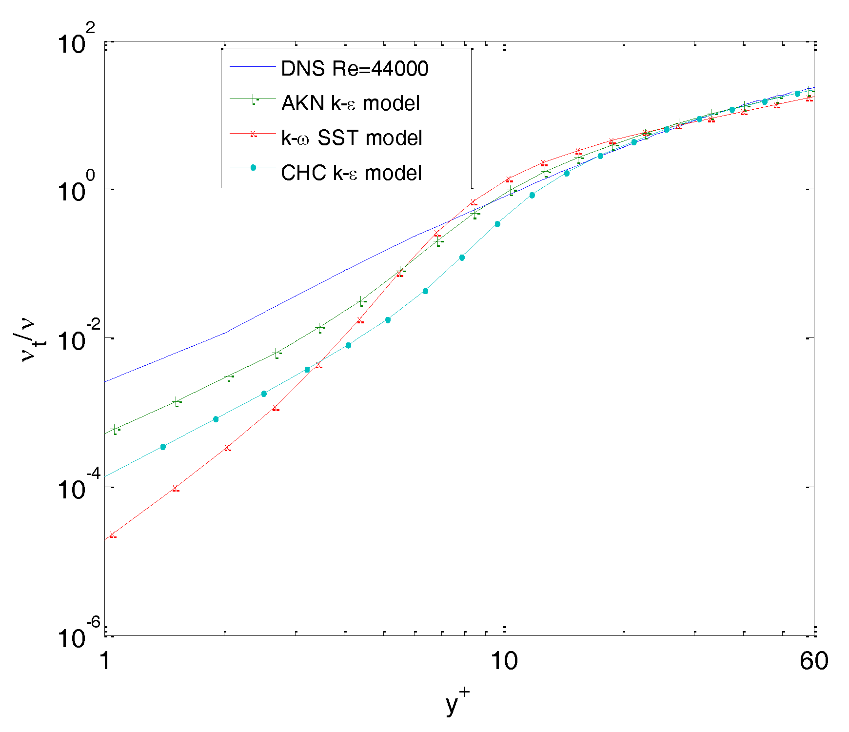
Turbulent transport is appreciable and dominantly contributes to concentration verification in the viscous sublayer. All LRN models (AKN, CHC, SST) under predicted the turbulent viscosity in this sublayer, and thus also under predicted the local mass transfer coefficient. The AKN model gave the best estimation of turbulent viscosity in the viscous sublayer.

(2)

The AKN model accurately predicted the Stanton number with a relative error of 6.54% while the SST and CHC models’ estimate of the Stanton number with relative errors was even greater than 40% for straight pipe flow at Re = 44,000. Moreover, the Stanton number predicted by the AKN model was less than that derived from the experience model of Berger and Hau with a relative error of 4–10%, in the region of 10,000 < Re < 100,000.

(3)

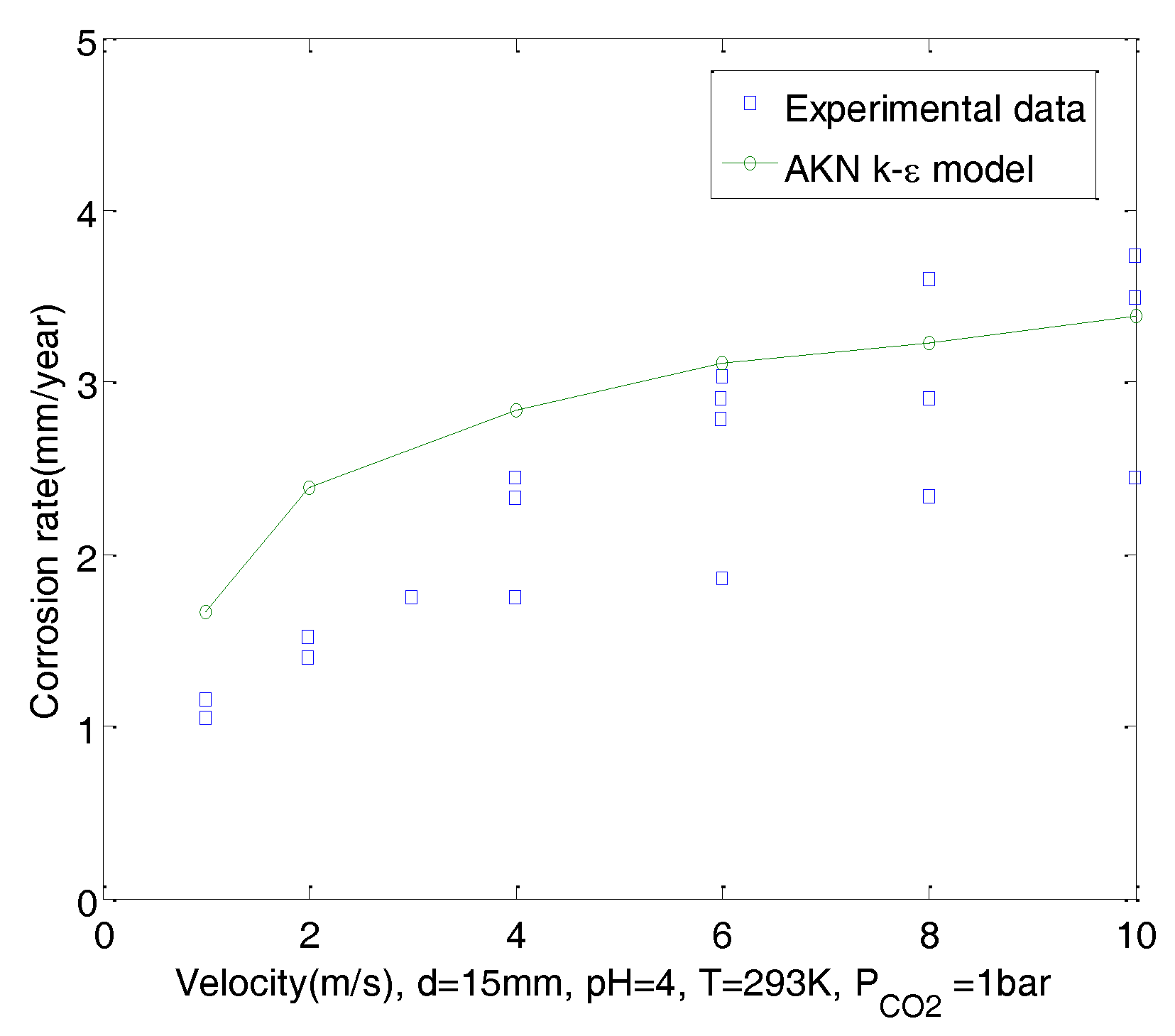
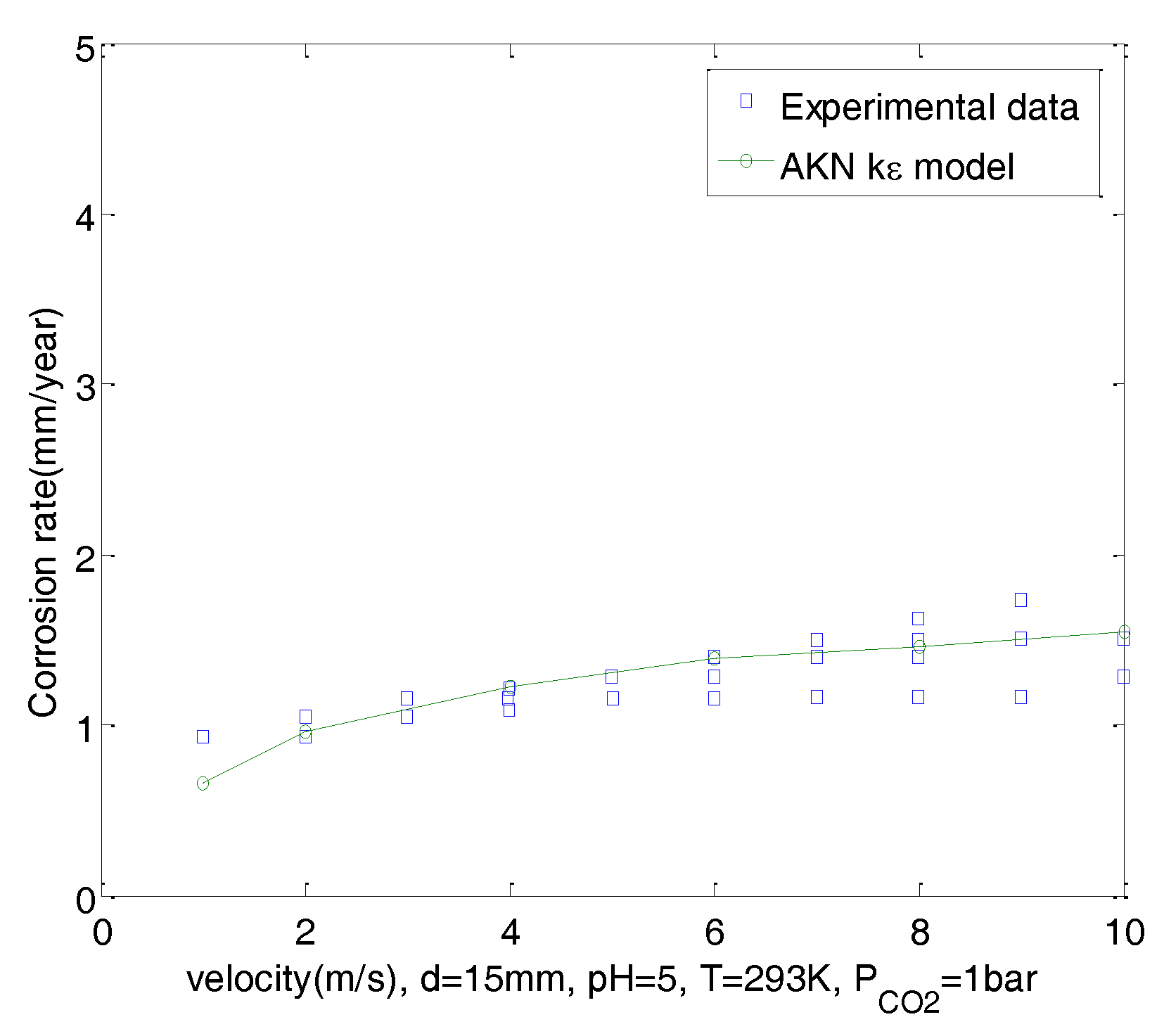
Predictions of CO₂ corrosion were made using UDFs and the AKN model for domains with 2D geometry under steady-state flow. Boundary conditions of corroded walls can be derived from the mixture potential, which was responsible for the charge balance of the corroded surface. Corrosion rates of CO₂ solutions in a straight pipe with d = 15 mm under pH = 4, 5 and 6, P_CO2 = 1 bar were predicted. Results show that predictions have good agreement with experimental data and correctly reflect the effect of velocity on the corrosion. Corrosion rates were not only more sensitive to change in flow at low pH than at high pH, but were also more sensitive to change in flow at low velocity than at high velocity.

(4)

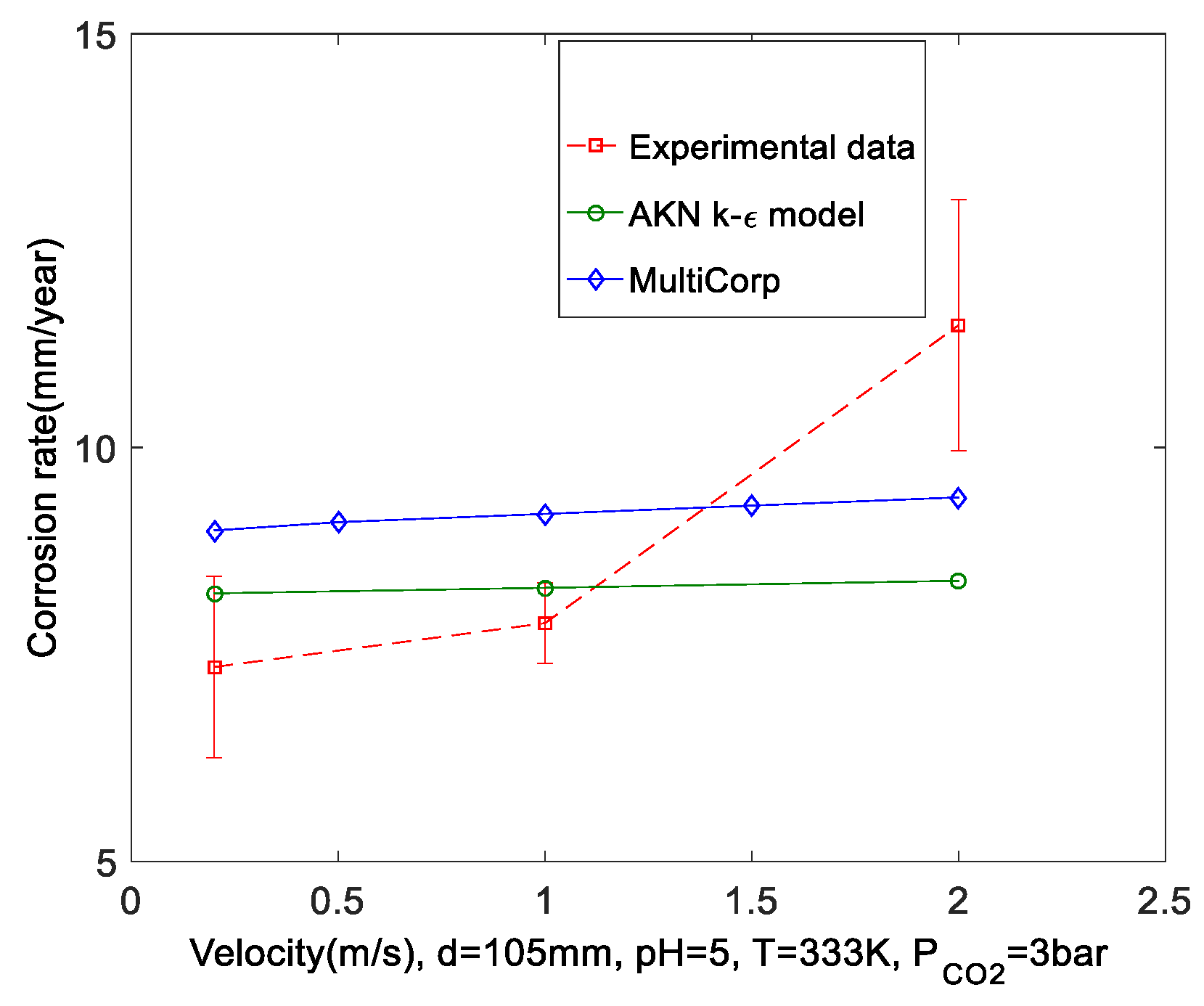
The corrosion rates of CO₂ solutions in a straight pipe with d = 25.4 mm under pH = 5, P_CO2 = 1 bar, U_m = 4 m/s, and T_K = 20–80 °C were predicted using the AKN model and compared with those derived using the Multicorp V5.2.105. Both codes correctly show that corrosion rates increase as temperature rises. However, the UDFs gave lower predictions than the Multicorp. Predictions of CO₂ corrosion in a straight pipe with d = 105 mm under pH = 5, P_CO2 = 3 bar, T_K = 333 K, U_m = 0.2–2 m/s were made and compared with experimental data and Multicorp data. Results show that the predictions are reasonable and close to Multicorp data. The predictions correctly show that corrosion rates do not vary greatly with change of velocity since the corrosion process was mainly controlled by the CO₂ hydration reaction, which is insensitive to velocity under the tested conditions.

(5)

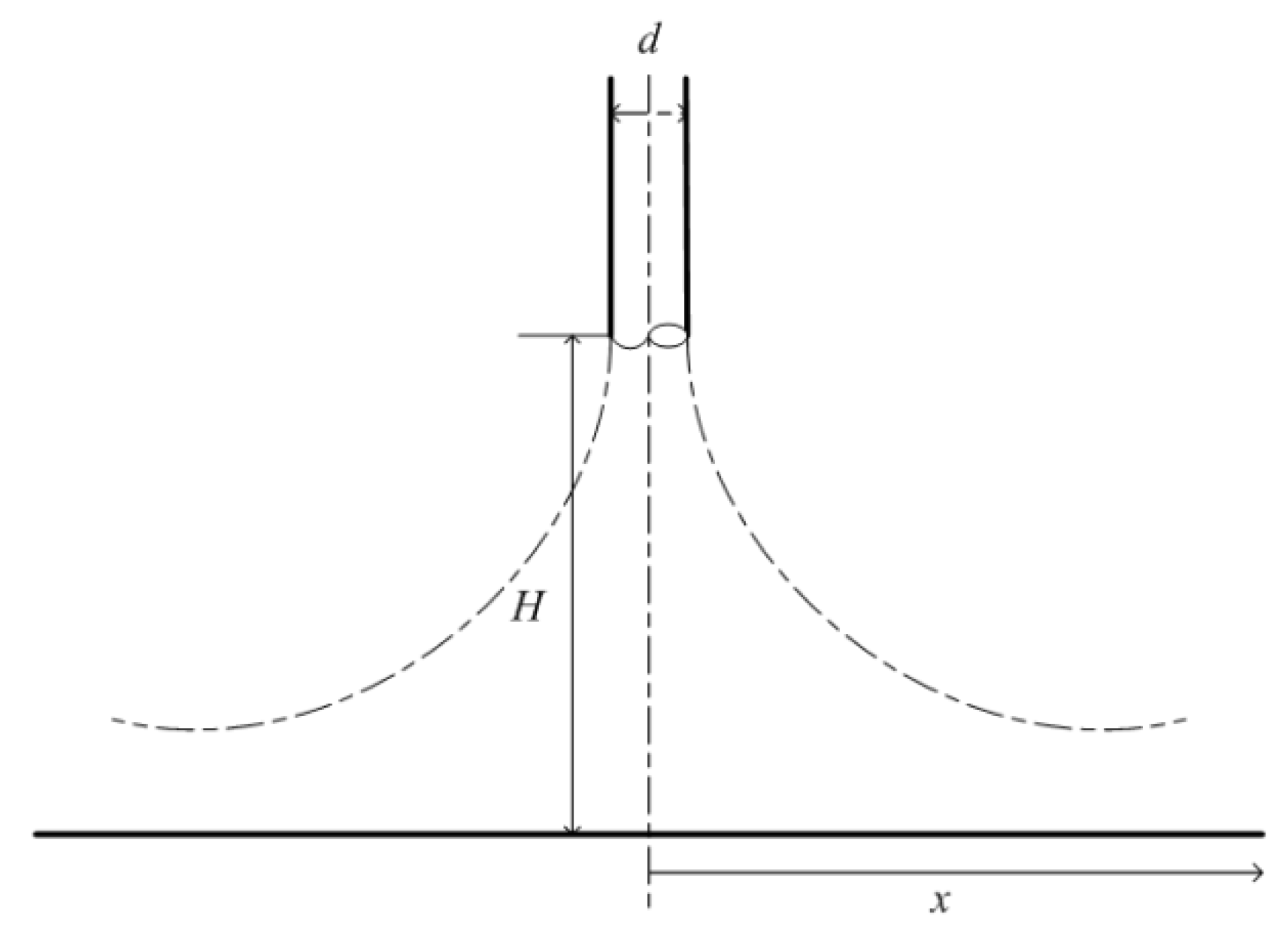
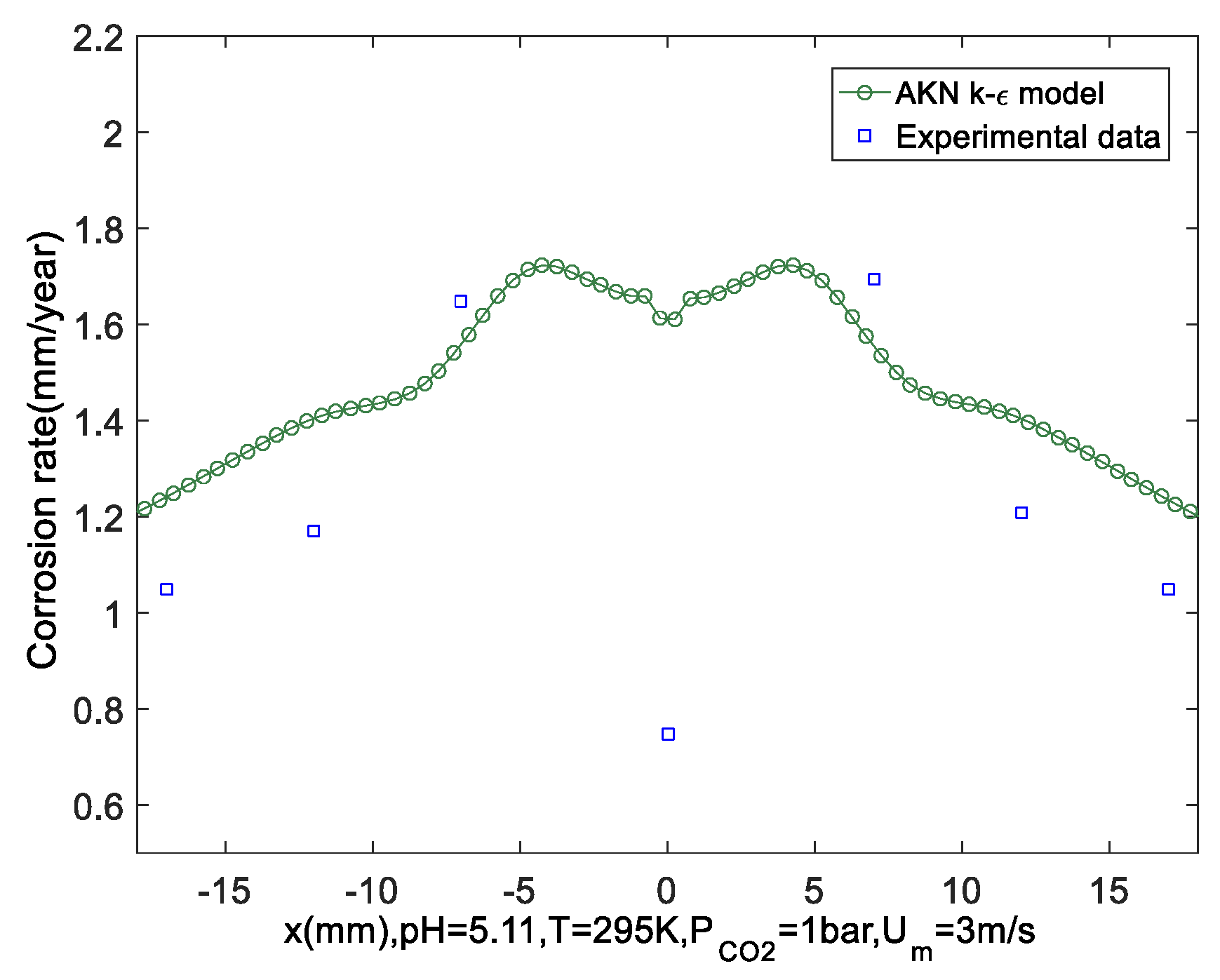
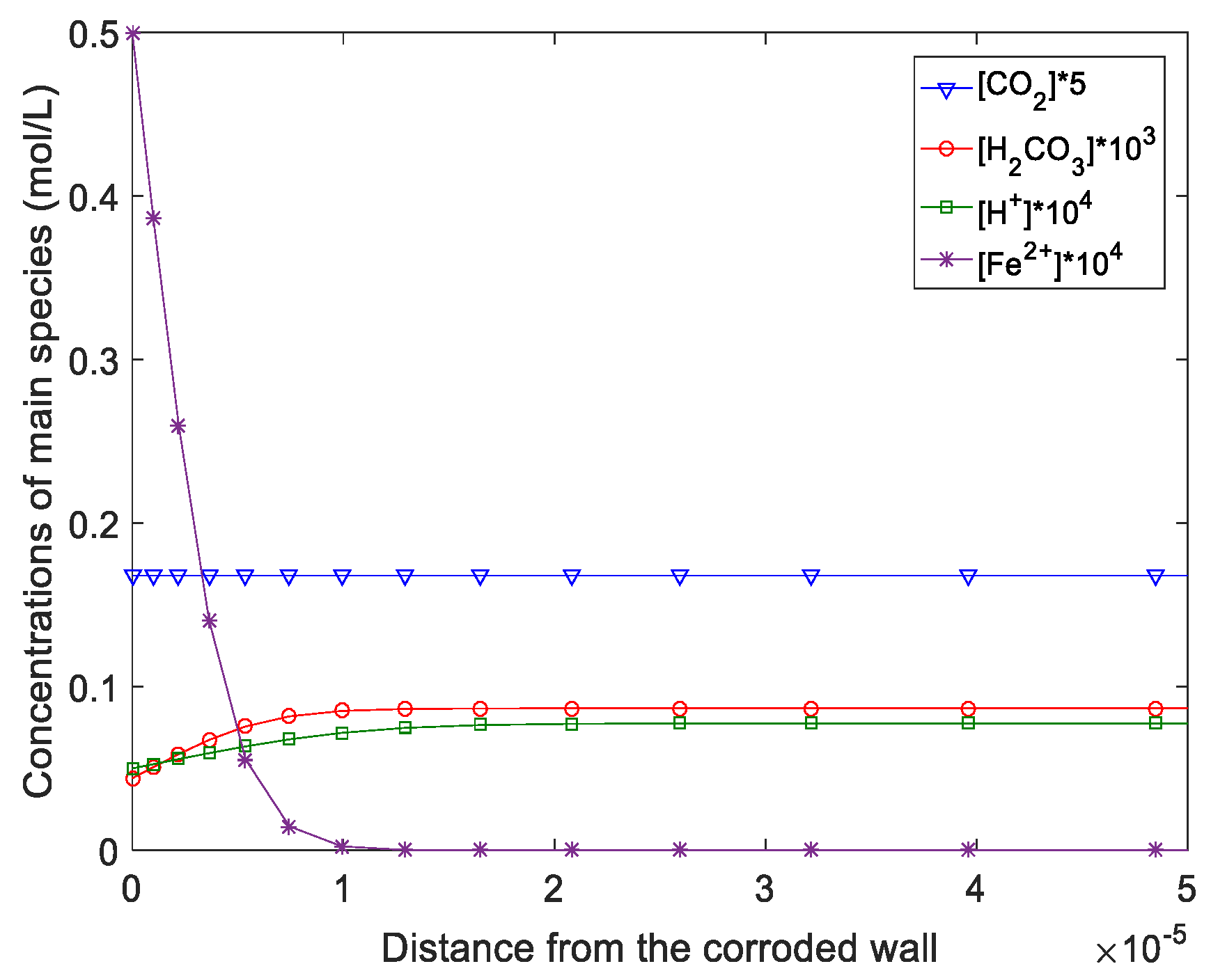
The flow and corrosion in a jet impinging were predicted by the AKN model. The results show that numerical predictions of the corrosion rate have good agreement with experimental data. The position with the most serious local thinning was around 0.6*d from the wall center in the jet impinging system. The concentration profiles of ions in solutions denote that H₂CO₃ plays a greater role in corrosion.

References

1. De Waard, C.; Lotz, U. Prediction of CO2 Corrosion of Carbon Steel; Corrosion/93; NACE International: Houston, TX, USA, 1993; p. 69. [Google Scholar]
2. De Waard, C.; Lotz, U.; Dugstad, A. Influence of Liquid Flow Velocity on CO2 Corrosion: A Semi-Empirical Model; Corrosion/95; NACE International: Houston, TX, USA, 1995; p. 128. [Google Scholar]
3. Jepson, W.P.; Stitzel, S.; Kang, C.; Gopal, M. Model for Sweet Corrosion in Horizontal Multiphase Slug Flow; Corrosion/97; NACE International: Houston, TX, USA, 1997; p. 11. [Google Scholar]
4. De Waard, C.; Smith, L.; Bartlett, P.; Cunningham, H. Modelling Corrosion Rates in oil Production Tubing; Eurocorr: Riva del Garda, Italy, 2001; p. 254. [Google Scholar]
5. De Waard, C.; Smith, L.; Craig, B.D. The Influence of Crude Oil on Well Tubing Corrosion Rates; Corrosion/03; NACE International: Houston, TX, USA, 2003; p. 3629. [Google Scholar]
6. Nešić, S.; Postlethwaite, J.; Olsen, S. An electrochemical model for prediction of corrosion of mild steel in aqueous carbon dioxide solutions. Corrosion 1996, 52, 280. [Google Scholar] [CrossRef]
7. Anderko, A.; McKenzie, P.; Young, R.D. Computation of rates of general corrosion using electrochemical and thermodynamic models. Corrosion 2001, 57, 202. [Google Scholar] [CrossRef]
8. George, K.; Wang, S.; Nešić, S.; de Waard, C. Modeling of CO2 Corrosion of Mild Steel at High Pressures of CO2 and in Presence of Acetic Acid; Corrosion/04; NACE International: Houston, TX, USA, 2004; p. 4623. [Google Scholar]
9. Sun, W.; Nešić, S. A mechanistic model of uniform hydrogen sulfide/carbon dioxide corrosion of mild steel. Corrosion 2009, 65, 291. [Google Scholar] [CrossRef]
10. Zheng, Y.; Ning, J.; Brown, B.; Nešić, S. Electrochemical model of mild steel corrosion in a mixed H2S/CO2 aqueous environment in the absence of protective corrosion product layers. Corros. Sci. 2014, 71, 316. [Google Scholar] [CrossRef]
11. Zheng, Y.; Ning, J.; Brown, B.; Nešić, S. Advancement in Predictive Modeling of Mild Steel Corrosion in CO2 and H2S Containing Environments; Corrosion/15; NACE International: Houston, TX, USA, 2005; p. 6146. [Google Scholar]
12. Nešić, S.; Li, H.; Huang, J.; Sormaz, D. An open source mechanistic model for CO2/H2S corrosion of carbon steel. In Proceedings of the NACE International Corrosion Conference & Expo, Atlanta, GA, USA, 22–26 March 2009. [Google Scholar]
13. Nordsveen, M.; Nešić, S.; Nyborg, R.; Stangeland, A. A mechanistic model for carbon dioxide corrosion of mild steel in the presence of protective iron carbonate films-Part 1: Theory and verification. Corrosion 2003, 59, 443. [Google Scholar] [CrossRef]
14. Song, F.M. A comprehensive model for predicting CO2 corrosion rate in oil and gas production and transportation systems. Electrochimi. Acta 2010, 55, 689. [Google Scholar] [CrossRef]
15. Berger, F.P.; Hau, K.F.F.L. Mass transfer in turbulent pipe flow measured by the electrochemical method. Int. J. Heat Mass Transf. 1977, 20, 1185. [Google Scholar] [CrossRef]
16. Nešić, S. Key issues related to modelling of internal corrosion of oil and gas pipelines–A review. Corros. Sci. 2007, 49, 4308. [Google Scholar] [CrossRef]
17. Kahyarian, A.; Singer, M.; Nesic, S. Modeling of uniform CO2 corrosion of mild steel in gas transportation systems: A review. J. Nat. Gas Sci. Eng. 2016, 29, 530. [Google Scholar] [CrossRef]
18. Li, X.; Hu, H.; Cheng, G.; Li, Y.; Xia, Y.; Wu, W. Numerical Predictions of Mild-Steel Corrosion in a H2S Aqueous Environment Without Protective Product Layers. Corrosion 2017, 73, 786. [Google Scholar] [CrossRef]
19. Nešić, S.; Adamopoulos, G.; Postlethwaite, J.; Bergstrom, D.J. Modelling of turbulent flow and mass transfer with wall function and low Reynolds number closures. Can. J. Chem. Eng. 1993, 71, 28. [Google Scholar] [CrossRef]
20. Nešić, S.; Postlethwaite, J.; Bergstrom, D.J. Calculation of wall-mass transfer rates in separated aqueous flow using a low Reynolds number κ-ε model. Int. J. Heat Mass Transfer. 1992, 35, 1977. [Google Scholar] [CrossRef]
21. Xiong, J.; Koshizuka, S.; Sakai, M. Turbulence modeling for mass transfer enhancement by separation and reattachment with two-equation eddy-viscosity models. Nucl. Eng. Des. 2011, 241, 3190. [Google Scholar] [CrossRef]
22. Wang, Y.; Postlethwaite, J. The application of low Reynolds number k-ε turbulence model to corrosion modelling in the mass transfer entrance region. Corros. Sci. 1997, 39, 1265. [Google Scholar] [CrossRef]
23. Hsieh, W.D.; Chang, K.C. Calculation of wall heat transfer in pipe expansion turbulent flows. Int. J. Heat Mass Transf. 1996, 39, 3813. [Google Scholar] [CrossRef]
24. Wang, S.J.; Mujumdar, A.S. A comparative study of five low Reynolds number k-ε models for impingement heat transfer. Appl. Therm. Eng. 2005, 25, 31. [Google Scholar] [CrossRef]
25. Gorji, S.; Seddighi, M.; Ariyaratne, C.; Vardy, A.E. A comparative study of turbulence models in a transient channel flow. Comput. Fluids 2014, 89, 111. [Google Scholar] [CrossRef] [Green Version]
26. Ansys. Fluent Theory Guide; Ansys: Canonsburg, PA, USA, 2015. [Google Scholar]
27. Kharaka, Y.K.; Gunter, W.D.; Aggarwal, P.K.; DeBraal, J.D. SOLMINEQ 88: A Computer Program for Geochemical Modeling of Water-Rock Interactions; US Geological Survey: Menlo Park, CA, USA, 1989.
28. Duan, Z.; Li, D. Coupled phase and aqueous species equilibrium of the H2O–CO2–NaCl–CaCO3 system from 0 to 250 °C, 1 to 1000 bar with NaCl concentrations up to saturation of halite. Geochim. Cosmochim. Acta 2008, 72, 5128. [Google Scholar] [CrossRef]
29. Bockris, J.O.M.; Drazic, D.; Despic, A.R. The electrode kinetics of the deposition and dissolution of iron. Electrochim. Ascta 1961, 4, 325. [Google Scholar] [CrossRef]
30. Wu, X.; Moin, P. A direct numerical simulation study on the mean velocity characteristics in turbulent pipe flow. J. Fluid Mech. 2008, 608, 81. [Google Scholar] [CrossRef]
31. Rao, V.V.; Trass, O. Mass transfer from a flat surface to an impinging turbulent jet. Can. J. Chem. Eng. 1964, 42, 95. [Google Scholar] [CrossRef]
32. Zhang, G.A.; Cheng, Y.F. Electrochemical characterization and computational fluid dynamics simulation of flow-accelerated corrosion of X65 steel in a CO2-saturated oilfield formation water. Corros. Sci. 2010, 52, 2716. [Google Scholar] [CrossRef]
33. Nešić, S.; Solvi, G.T.; Enerhaug, J. Comparison of the rotating cylinder and pipe flow tests for flow-sensitive carbon dioxide corrosion. Corrosion 1995, 51, 773. [Google Scholar] [CrossRef]
Figure 1. Axial velocity predicted using LRN models vs. DNS data [30].
Metals 08 01001 g001
Figure 2. Turbulent viscosity predicted using LRN models vs. that derived from DNS data [30].
Metals 08 01001 g002
Figure 3. Predicted and empirical Stanton number varying with Reynolds number.
Metals 08 01001 g003
Figure 4. The jet impinging flow.
Metals 08 01001 g004
Figure 5. Predicted Sherwood number vs. experimental data [31].
Metals 08 01001 g005
Figure 6. Schematic diagram of a jet impinging.
Metals 08 01001 g006
Figure 7. Corrosion rate obtained using the AKN model vs. experiment data [33] with pH = 4, T = 293.15 K, PCO2 = 1 bar.
Metals 08 01001 g007
Figure 8. Corrosion rate obtained using the AKN model vs. experiment data [33] with pH = 5, T = 293.15 K, PCO2 = 1 bar.
Metals 08 01001 g008
Figure 9. Corrosion rate obtained using the AKN model vs. experiment data [33] with pH = 6, T = 293.15 K, PCO2 = 1 bar.
Metals 08 01001 g009
Figure 10. Corrosion rate obtained using the AKN model vs. Multicorp V5.2.105 data with pH = 5, PCO2 = 1 bar, Um = 4 m/s.
Metals 08 01001 g010
Figure 11. Corrosion rate obtained using the AKN model vs. experiment data [8] and Multicorp V5.2.105 data with pH = 5, T = 333.15 K, PCO2 = 3 bar.
Metals 08 01001 g011
Figure 12. Flow filed distributions of the jet impinging flow with Um = 3 m/s, θ = 90°.
Metals 08 01001 g012
Figure 13. Corrosion rate obtained using the AKN model vs. experiment data [32] with pH = 5.11, T = 22 °C, Um = 3 m/s, PCO2 = 1 bar, θ = 90°.
Metals 08 01001 g013
Figure 14. Predicted concentrations of main species vs. the normal distance from the corroded wall on the position (x = 0.6 d, y = 0, z = 0).
Metals 08 01001 g014