Evaluation of the Thermal Comfort and Energy Demand in a Building with Rammed Earth Walls in Spain: Influence of the Use of In Situ Measured Thermal Conductivity and Estimated Values

Abstract

This paper describes the influence of thermal parameters—conductivity, transmittance, and thermal mass—in the estimation of comfort and energy demand of a building with rammed earth walls, and consequently, the compliance with standards. It is known that nominal design data does not match in situ measured values, especially in traditionally constructed buildings. We have therefore monitored a room in a building with rammed earth walls, designed a computerised model, and compared four different alternatives where we have changed the value for the thermal conductivity (in situ vs. estimated) and the consideration of thermal mass. When we then analyse the compliance with the Spanish energy saving code, using measured values would result in lower differences with the standards’ limits and even comply with the global thermal transmittance (K-value) requirement. This would mean a more realistic approach to the restoration of traditional buildings leading to the use of thinner and more suitable insulation and retrofitting systems, encouraging the use of rammed earth in new buildings, and therefore reducing the carbon footprint due to materials used in construction. Results show that the building model that uses in situ values and considers thermal mass (S1) is closer to reality when assessing thermal comfort. Finally, using nominal data would result in requiring 43% more energy in the selected winter period and 102% more energy in the selected summer period to keep the same comfort conditions as in the alternative where measured values are used.

1. Introduction

Understanding the thermal behaviour of materials is essential to achieve a correct energy evaluation of buildings, their demands, and the environmental impact due to the consumption of resources. A report from the International Energy Agency (IEA) states that, in 2019, the building sector causes two-fifths of the total CO₂ emissions, being responsible for over one-third of the global final energy consumption [1], having risen in the last years [2]. 11% of these CO₂ emissions resulted from manufacturing building materials like steel, cement, and glass. Thus, the use of materials that have minimal impact on the environment during their lifecycles will contribute to mitigate the effects of climate change. One of these materials is earth, and although its awareness in construction is high, its current use remains low [3].

In order to achieve an efficient use of materials in buildings, governments of many countries improve energy and environmental demands in construction standards. However, another report from the IEA revealed that in 2019, almost two out of three countries did not have mandatory building energy codes [4]. In Spain, the Technical Code of Buildings is the standard that establishes the requirements that buildings must meet, and since 2006, the document about Energy Saving aims to ameliorate the situation by ensuring a proper use of the energy in buildings [5]. There is an application included in the Spanish Code that gives theoretical parameters of materials that can be used to execute approximate calculations and can help us analyse the behaviour of the building once it is in use [6].

To quantify the influence of materials on the energy efficiency of buildings it is also necessary to consider the methodology that is employed to determine the physical parameters that define those materials. The use of appropriate values in relation with building analysis and its consequences in the compliance of energy saving requirements is an issue that is constantly under discussion among professionals. Previous research has determined that nominal design data does not match in situ measured values, especially in traditionally constructed buildings.

Table 1. Disparities found in literature review: estimated and measured U values in uninsulated and no air gap walls.

Paper	Technical Specification of the Wall (Int-Ext)	Thickness (m)	U-Value (W/m2K)
			Estimated	Measured
[7]	Plaster on lath + solid sandstone wall + ashlar	0.60	1.20–1.50	1.00
[8]	Mortar + brick + plaster	0.30	1.30–2.20	1.30
	Mortar + brick + bare painted brick	0.30	1.30–2.40	1.20
[9]	thermal plaster + thermal block + plaster	0.45	0.32	0.56
[10]	gypsum plastering + brick	0.31	1.60–2.39	1.16 ± 0.06
[11]	Several cases (all solid walls: 40 brick walls and 18 stone walls)	- 1	2.10	1.30 ± 0.4
[12]	plastering + solid brick	0.25	2.07	1.48
[13]	plaster + hollow clay brick + solid concrete block + hollow concrete block + plaster	0.50	0.42–1.55	0.68 ± 0.07
	plaster + tuff block + plaster	0.46	0.99–2.23	0.80 ± 0.09
[14]	lime and cement plastering + brick	0.25	2.24	1.57
[15]	plaster + solid brick	0.70	0.88	0.52
	plaster + solid brick	0.52	1.12	0.78
[16]	Gypsum mortar + rammed earth + cement mortar	0.50	1.58	0.35
[17]	Plaster + rammed earth + mortar	0.72	1.01	0.58

¹ several walls with different thicknesses were studied in this paper.

describes the differences between the estimated and the measured thermal transmittance—or U value—found in research where the subject of study was uninsulated walls with no air gap [7,8,9,10,11,12,13,14,15,16,17]. All the measured transmittance values were calculated using the average method, as per the International Organization for Standardization ISO 9869 [18], and some of them include an estimation of the uncertainty of the results.

If we focus on earth constructions, other researchers have also performed both in situ monitoring and energy simulations during the last decade aiming to study the thermal behaviour of this material in buildings. A review of all these papers can be found in [19,20], and the conclusions indicate that:

• Exploring the differences between estimated and measured data is necessary to characterise the thermal properties of earthen structures, and it is much more accurate if it is related to a specific climatic zone;
• A common methodology to monitor earth buildings should be established;
• Occupation and activity in the building is usually not studied, and it can highly influence the results;
• The adaptative model as per the American Society of Heating, Refrigerating and Air-Conditioning Engineers (ASHRAE), standard number 55, is the most common to describe thermal comfort, and the (ISO) 9869 to characterise thermal parameters of walls;
• In order to study different parameters in buildings via simulations, the validation of the numerical model is necessary.

In [16,21] the impact of using theoretical and measured values regarding the compliance of the Spanish code is described. This is especially important in our case, as both conclude that measured values provide more accurate simulation results and that there should be a review in the demands of regulations applied to traditional architecture. Nevertheless, it is assumed that uncomfortable temperatures usually happen below the comfort limit, requiring insulation to improve their energy and thermal performance in Winter, as has been stated in many papers [22,23,24,25,26,27,28]. This would lead to the need of retrofitting, not only to comply with energy codes, but also to reduce the building’s overall energy demand. A review of criteria and methods in the energy retrofitting of traditional buildings can be found in [29]. It concludes that to carry out an accurate evaluation of the need of retrofitting, it is essential to select an appropriate simulation software and increase the gathering of measured data such as properties of materials and indoor climate conditions. Also, it affirms that retrofitting is necessary to preserve this kind of building. Another study in Iran revealed through simulation analysis that traditional-indigenous houses had a lower heat transfer than contemporary houses, leading to a lower energy consumption [30]. Finally, it can be concluded that building energy restoration presents a vast potential if the right policies are implemented. Although different measures to reduce or save energy in buildings have been proposed, there is still a need for researchers to develop other models to solve this same issue [31]. All these ideas explain the great possibilities of traditional construction in a world that moves towards an ecological transition and sustainable development.

The novelty of this work is to compare the influence between using measured values of thermal conductivity of a rammed earth wall in a traditional building, obtained in past research [17], and estimated values found in the Spanish code, on the indoor thermal comfort and on the energy demand. Also, the degree of compliance with the Spanish code and energy certification can be studied depending on which value is used, as was also explained in [11], referred to UK regulation. Finally, to achieve an accurate description of the thermal inertia that a wall can provide, the most important parameter is thermal conductivity [32,33]. Therefore, the simulations described in this paper have been executed considering the thermal conductivity and consequently the effect of thermal inertia in comfort, energy demand, and compliance with standards.

The paper is organised as follows. Section 2 explains the building characteristics, monitoring, simulation and the methodology, tools, and reference parameters used to analyse the data. Consequently, in Section 3 we compare the different versions of the building model through four correlation methods, and then we present the results for thermal comfort and energy demand. This leads to a validation of one of the alternatives, which is discussed in Section 4 together with the compliance with the Spanish energy saving code. Finally, Section 5 shows the conclusions of the research, summarising the main ideas of the work that demonstrate the convenience of using measured values to design a proper energy model of a building with rammed earth walls.

2. Materials and Methods

Research is executed the following way. First, we recorded the indoor temperature and relative humidity parameters in a room located in a house built with uninsulated traditional rammed earth walls. Secondly, we have modelled and carried out simulations of the building using estimated and in situ measured thermal conductivity and transmittance parameters, considering the mass of the wall. Lastly, we have determined the influence of using different values for the thermal conductivity and considering the thermal mass of the wall in the thermal comfort and the energy demand, using a model where these are the only parameters that change, as well as to comply with energy building code requirements.

This section is organised starting with the analysis of the case study (Section 2.1), where we describe the building and the in situ experimentation, and then we explain the building simulations carried out with DesignBuilder (Section 2.2) and all the details that we have considered to execute them and to analyse the results. These details are the information that has been introduced in the software, the simulation variables, the correlation of the different versions of the model with measured values, the thermal comfort analysis and the energy demand analysis. At the end of the section, we also include an explanation of the compliance with the Spanish energy saving code using a different simulation software (Section 2.3).

2.1. Case Study Analysis

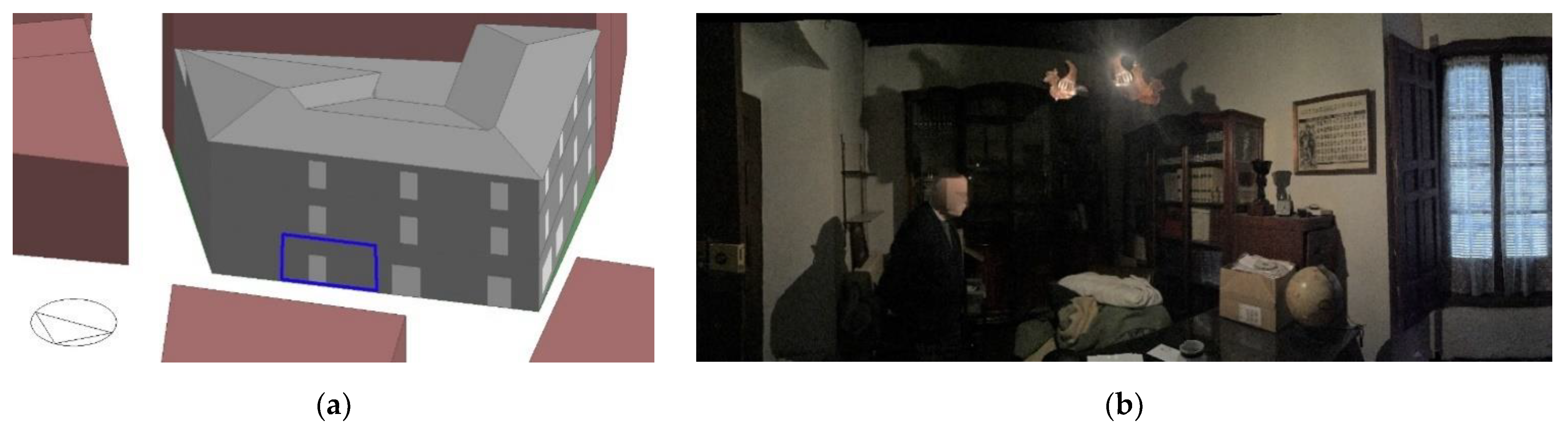
2.1.1. Description of the Studied Building and Room

The building is located in a dry Mediterranean climate—classified as BSk-Csa in the Köppen-Geiger climate classification [34]—in the village of Campo de Criptana (Ciudad Real, Spain). Winters are cold, reaching temperatures of −5 °C, while summers are hot and semi-arid, when temperatures get up to 40 °C.

The building has a total built area over 800 m² and a net usable area over 600 m², three stories high and envelopes consisting of 70-cm-thick rammed earth walls in the ground floor, and 54 cm thick in upper floors, with an internal gypsum plaster and an external cement render. It was built in the early 20th century. The monitored room (15 m²) is located on the ground floor below a living room, on the ground floor, containing a heating system that is constantly operative, no cooling devices, a 1.00 × 1.80 m window and is completely furnished as a home office (Figure 1 and Figure 2). The room was selected because of its orientation (North), great wall-to-window ratio, and null occupancy to examine the influence of the wall properties in the indoor environmental conditions, minimising the impact of other variables.

2.1.2. In Situ Experimentation and Survey Research

We have carried out several types of tests and surveys to analyse the building:

• We have monitored the environmental conditions of the described room, recording the indoor temperature and humidity and outdoors dry-bulb temperature and relative humidity values;
• We have collected information about the use of the building through surveys to the users every six months (October–March and April–September).
• We have characterised the thermal conductivity and transmittance of the wall using the ISO 9869 standard [18] (already published in the previous research paper [17]).

The monitoring system is the same that was used in [17]. The sensor is a SHT75 (Sensirion AG, Stäfa, Switzerland), with accuracy ±0.3 °C and ±1.8%, while external conditions like temperature, relative humidity, and wind speed and direction were measured using a weather station, model FSW 20 (PCE Ibérica S.L., Tobarra, Spain) located in the same village. The period of monitoring is from 14 December 2017–15 December 2018 (Figure 3).

In addition, we performed a blower door test of the room to determine the air infiltration, consequently analysing the permeability of the room. The surveys to the users of the building were designed considering previous research projects [35,36], and consisted in the collection of data about the activity in the room (setpoint temperature of the heating device, ventilation, and the general use of the room).

2.2. Building Energy Performance Simulations

We have conducted simulations of the building using DesignBuilder software, version 7.0. It is an interface for simple building modelling and the export of data to the Energy Plus calculation engine. It allows us to check the performance of building’s features like passive design, installations, daylighting, CFD (Computational Fluid Dynamics), as well as material costs and optimisation, all through energy simulations. Input is introduced at four levels: location, building, floor, and room.

In our case, we introduced all the data that was collected through in situ tests and surveys, completing the unknown information about building elements with estimated data that can be found in the Spanish code [5,6,37].

Table 2. General information introduced in DesignBuilder and used in all simulations. In bold: actual data from tests/surveys.

			Building Level	Room Level: Office (Ground Floor)
Activity	Occupancy	Density	0.03 people/m2	Unoccupied
		Schedule	Weekdays: 100% 0–8 h; 25% 8–16 h; 50% 16–24 h Weekends: 100% 0–24 h	Unoccupied
		Metabolic	117.2 W/person	Unoccupied
	Environmental control	Heating	Setpoint: 20 °C Set back: 17 °C	Setpoint: 20 °C Set back: 18.5 °C
		Cooling	Setpoint: 25 °C Set back: 27 °C	No cooling system
	Office equipment	Power density	4.40 W/m2	No activity
		Schedule	50% 0–1 h; 10% 1–8 h; 30% 8–18 h; 50% 18–19 h; 100% 19–24 h	No activity
Construction	External walls		0.01 m gypsum plaster + 0.70 m rammed earth 1,2 + 0.02 cement mortar
	Pitched Roof		0.05 m plywood + 0.15 m EPS (Expanded polystyrene insulation) + 0.01 m PU (Polyurethane) + 0.025 m air gap + 0.06 m clay tile
	Partitions		0.01 m gypsum plaster + 0.12 m adobe 2 + 0.01 gypsum plaster
	Ground floor		0.15 m cast concrete + 0.15 m gravel
	Internal floor		0.01 m gypsum plaster + 0.08 m plywood + 0.01 gypsum plaster + 0.03 m clay tile
	Airtightness		Rate at 50 Pa: 10.49 h−1
Openings	Glazing		4 mm + 12 mm air + 4 mm	4 mm
	Frame		PVC (polyvinyl chloride)	Wood
Lighting	Schedule		50% 0–1 h; 10% 1–8 h; 30% 8–18 h; 50% 18–19 h; 100% 19–24 h	No lighting (no activity)
HVAC 3	Heating	Fuel	Oil	Oil
		Schedule	October–May: 17 °C 0–8 h; 20 °C 8–24 h	October–May: 18.5 °C 0–7 h; 20 °C 7–15 h; 18.5 °C 15–24 h
	Cooling	Fuel	Electricity	No cooling system
		Schedule	June–September: 27 °C 0–8 h; 25 °C 16–24 h

¹ 0.54 m rammed earth in the upper floor. ² Thermal properties change depending on the simulations, which are detailed in Table 3. ³ Heating – Ventilation – Air Conditioning.

is a summary of all this information, differencing between the data that was introduced at a building level from the data which was studied in the monitored room (real information is highlighted). The details for the location were filled out using the parameters that were measured by the weather station during the same year of the tests and surveys (2018).

The following details must be mentioned:

• We have used the Conduction Transfer Function (CTF) solution algorithm, which only considers heat transfer. Previous research compared three different methods to assess energy performance: CTF, HAMT (Heat and Moisture Transfer) and EMPD (Effective Moisture Penetration Depth), and concluded that for a hot and dry climate, the CTF is the best option for building energy simulation analysis [38];
• Ground monthly temperatures were not measured. According to the program’s manual: “a reasonable default value of 2 °C less than the average monthly indoor building temperature is appropriate for large buildings”. Therefore, this was introduced in the location level of the software;
• The density of the rammed earth wall has not been determined in situ, so we have used a density of 1885 kg/m³, which is the mean value we can find in the Technical code of Spain [6] and it is in accordance with values provided by different characterisation studies of this type of construction [39,40,41]. Nevertheless, we have also analysed the effect of using different values for the density of the earth in the wall on the correlation between the model and the actual building.

2.2.1. Simulation Variables

We have simulated four different alternatives changing the thermal parameters of conductivity and the consideration of thermal mass by the software: S1, S2, S3, and S4. This has been done by filling out thermal bulk properties for thermal conductivity, specific heat, and density when we wanted the software to consider thermal inertia, or by specifying a thermal resistance value, o R-value, when we did not want the software to did not consider it.

Therefore, S1 and S2 consider the thermal inertia of the wall and the value that changes is the thermal conductivity: S1 uses the measured thermal conductivity—or λ-value—of rammed earth obtained from a previous study [17], and S2 uses the estimated thermal conductivity as specified in the Spanish code [6]. On the other hand, S3 and S4 do not consider the thermal inertia of the wall. S3 uses the measured λ-value for rammed earth to calculate an R-value, and S4 uses the estimated λ-value to calculate the R-value of the wall. All this is detailed in

Table 3. Simulation alternatives: external walls and internal partitions ^1..

	S1 in Situ λ	S2 Estim. λ	S3 in Situ λ—R	S4 Estim. λ—R
Thermal mass consideration	YES		NO
λ-value (W/mK)	0.46	1.10	-	-
Specific Heat (J/kgK)	1000		-	-
Density (kg/m3)	1885		-	-
R-value (m2 K/W)	-	-	1.52 (partitions: 0.26)	0.64 (partitions: 0.11)

¹ information is not detailed in the software whenever the hyphen sign appears.

.

2.2.2. Correlation between S1 to S4 Alternatives and Measured Values

The correlation between simulations and monitored data is displayed through four different methods. These will indicate which alternative S1 to S4 is closer to the actual measured values, therefore validating the results of one of those alternatives. The four methods are the following:

• Coefficient of determination (R²), which is used in statistics to predict future results or to prove a hypothesis. In our case, it is employed to determine the quality of the model in DesignBuilder and the difference between the model and the actual air temperature in the measured spaces, as can be found in previous research [42,43,44]. We have analysed periods of 24 h, 72 h and a week, in Winter and in Summer. We have not used longer periods as we have considered that the R² value is too low;
• Using graphs that show short periods of time: a week in Winter and a week in Summer. These weeks are the same that have been used for the R² coefficient;
• Determination of the RMSE (Root-mean-square error) as found in previous research [42,43,44], and the maximum temperature deviation, indicating the amount of error between simulated and measured values;
• Comparison of results during a month in Summer, using the adaptative model described in the ASHRAE 55 [45].

The periods of time for each of these methods is described in

Table 4. Periods of time used to analyse the correlation between S1 to S4 alternatives and measured values.

	R2 Correlation	Graphical Correlation	RMSE and Max T. Deviation	Adaptative Model
24 h	8 January 2018 and 29 July 2018	-	8 January 2018 and 29 July 2018	-
72 h	8–10 January 2018 and 29–31 July 2018	-	8–10 January 2018 and 29–31 July 2018	-
One Week	8–14 January 2018 and 25–31 July 2018		-
One month	-		July 2018

. In the first three methods, the analysis parameter has been the indoor dry-bulb temperature as it was the parameter that was measured for the whole period and that affects both comfort and energy demand of the room In the fourth method we have used the indoor operative temperature, which is the mean temperature between air temperature and radiant temperature. As we did not monitor radiant temperature, so the in situ value in the last method has been calculated as the mean value between indoor dry-bulb temperature and surface temperature of a wall in the room.

2.2.3. Comfort Analysis

To analyse comfort inside the room we have used the adaptative model as per ASHRAE 55 [45]. This standard affirms that we must consider the indoor operative temperature and the model can only be used in naturally conditioned environments where no cooling or heating devices are in operation, occupants can adapt their clothing and the prevailing mean outdoor temperature is between 10 °C and 33.5 °C.

Accordingly, in our case the in situ measurements will only be valid for the summer period when no cooling devices were used. To analyse comfort during the winter period, we have carried out simulations with no heating system. Moreover, as the prevailing outdoor temperature is always below 10 °C during Winter, the 80% acceptable limits have been extended horizontally as can be seen in similar research [46]. This indicates that the minimum comfort operative temperature is always 17.4 °C (the maximum being 20.9 °C).

The limits for thermal comfort are defined in Figure 5-8 of the ASHRAE 55 standard, “Acceptable operative temperature t_o ranges for naturally conditioned spaces”. The equations to calculate indoor comfort are as follows:

T_ioc (°C) = 0.31 T_po + 17.8

(1)

T_iou (°C) = 0.31 T_po + 21.3

(2)

T_iol (°C) = 0.31 T_po + 14.3

(3)

being T_ioc the optimum comfort indoor operative temperature, T_iou the upper 80% acceptability limit, T_iol the lower 80% acceptability limit, and T_po the prevailing outdoor temperature. The ASHRAE standard specifies that the T_po shall be based on no fewer than 7 and no more than 30 sequential days prior to the day in question, being a simple arithmetic mean of the mean daily outdoor air temperatures of all the sequential days. In 2006, De Dear proposed a weekly mean temperature arguing that it represents a more independent variable for input than the default monthly mean [22]. Thus, as we have only studied the simulated alternatives for a week in winter and a week in summer, comfort analysis will be done using the following equation to calculate the prevailing outdoor temperature:

T_po (°C) = 0.34T_(day1) + 0.23T_(day2) + 0.16T_(day3) + 0.11T_(day4) + 0.08T_(day5) + 0.05T_(day6) + 0.03T_(day7)

(4)

being T_(day1) the mean outdoor temperature of the day before to the day in question, and T_(day7) mean outdoor temperature seven days before to the day in question.

2.2.4. Energy Demand Analysis

The energy demand is also studied using the simulation results. It can be described as the amount of energy required to keep thermal comfort, depending on the climate, the use of the room and its net usable area, the envelope’s characteristics, and solar radiation. Again, we have only examined the results for the periods of time of a week in Winter and a week in Summer that were studied as mentioned in Section 2.2.2.

To analyse it we have used the mean monthly temperature comfort values for winter 2018 and summer 2018 as the setpoint (optimum temperature calculated with Equation (1) and set back (setpoint temperature to be used at night-time, weekends, and other holidays during the heating season, calculated with Equation (2) -Summer- or Equation (3) -Winter-) that the building should reach to achieve comfort. These are:

• Winter: setpoint = 20.9 °C; set back = 17.4 °C
• Summer: setpoint = 26.5 °C; set back = 30 °C

Furthermore, we have used different schedules for the HVAC (Heating–Ventilation–Air Conditioning) than those described in Table 2. Here, Heating and Cooling systems use a time schedule “always on”. This means that when the room falls below the setpoint operative comfort temperature in winter or exceeds setpoint operative comfort temperature in summer, it will turn on. This way, we will be able to analyse the total energy demand of the room during both periods of time and compare which of the four alternatives S1 to S4 would require less energy to achieve optimum comfort.

2.3. Compliance with the Spanish Energy Saving Code

We have studied this compliance for the versions used in S1 and S2, using a Spanish software called “CE3X” (Certificación Energética de Edificios) that has been developed by Efinovatic and the Spanish National Centre for Renewable Energies (CENER). The use of the CE3X software in the study provides a perspective of the transfer of the regulations to the construction reality. CE3X is officially accepted and is historically the most widely used by professionals and even some BIM (Building Information Modelling) project management tools, given its simplified and operational nature. Thus, this software can be employed as an energy certification tool for existing and new buildings as well as to describe the degree of compliance with the Spanish Technical Code for energy saving [47].

In this program, a model of the whole building is designed without using graphical tools, which leads to a simplified layout of the building that did not consider the terrace on the upper storey, the unevenness of the street and the buildings that surround it (not being affected by shades). Heating and cooling devices were filled out with default values, specifying only the actual source of energy (fuel for heating and electricity for cooling). Moreover, this software describes the thermal bulk properties of materials (thermal conductivity, density and specific heat) but it does not give the option about thermal mass consideration as DesignBuilder did, so we have only compared the results for the alternatives S1 and S2.

As we are studying the whole building in a different simulation software, the results will be presented in the discussion section.

3. Results

The results are presented in two sections: first, the correlation between the four simulation alternatives and the monitored building (Section 3.1); secondly, we have used this correlation analysis to examine thermal comfort and energy demand in each of the alternatives, aiming to reveal which of them would give better results (Section 3.2).

3.1. Correlation between S1 to S4 Alternatives and Measured Values

3.1.1. R² Correlation

Table 5. R² correlation between measured and the simulated dry-bulb temperature in simulations 1 to 4. In bold: simulated values that are closer to the measured temperatures.

Period	Winter (January)				Summer (July)
	Mass (M)		No Mass (NM—R)		Mass (M)		No Mass (NM—R)
	S1: λ in Situ	S2: λ Estim.	S3: λ in Situ	S4: λ Estim.	S1: λ in Situ	S2: λ Estim.	S3: λ in Situ	S4: λ Estim.
24 h	0.91	0.87	0.87	0.76	0.98	0.97	0.97	0.96
72 h	0.81	0.72	0.75	0.65	0.90	0.84	0.89	0.88
One week	0.61	0.56	0.58	0.52	0.78	0.85	0.52	0.50

shows the R² correlation between measured and the simulated dry-bulb temperature in the room for January and July 2018. The periods of one day, three days, and one week (described in Section 2.2.2) have been chosen examining the dry-bulb temperature graphs, taking those moments when measured and simulated values were similar. Correlation is always higher when the thermal mass of the wall is considered, and almost always when we use the results for S1. The table shows this fact highlighting in bold the simulated values that are closer to the measured temperatures.

On the other hand,

Table 6. R² correlation between measured dry-bulb temperature and simulation 1 (λ in situ, Mass) depending on density (ρ).

Period	Winter (January)		Summer (July)
	ρ = 1885 kg/m3	ρ = 2500 kg/m3	ρ = 1885 kg/m3	ρ = 2500 kg/m3
24 h	0.91	0.91	0.98	0.98
72 h	0.81	0.81	0.90	0.90
One week	0.61	0.61	0.78	0.78

shows the effect of using different values for the density of the earth in the wall explained through the R² correlation between measured dry-bulb temperature and values in S1. As we can see, results remain unchanged.

3.1.2. Graphical Correlation

Figure 4a,b shows the Indoor Air Temperature (T_ia, in °C) of one week in Winter (8–14 January 2018) and one week in Summer (25–31 July 2018), in the studied room. Both figures show the effect of considering thermal mass, and it is more evident in the summer period, when temperatures in S1 and S2 are much more stable than those in S3 and S4. Also, both graphs show that the temperature in S1 is closer to the measured values.

Additionally, Figure 5a,b show the Relative Humidity (RH, in %) of the same periods of time. Although the RH is mostly the same in the four simulations, these graphs are shown to demonstrate that the pattern of moisture between the simulated and the actual environment is very similar. All figures show the results of the measured values and the four simulations.

3.1.3. RMSE and Maximum Temperature Deviation

The RMSE for the different periods is described in

Table 7. Root mean square error (RMSE) between in situ air temperature measurements and simulations in °C. In bold: simulated values that are closer to the measured temperatures.

Period	Winter (January)				Summer (July)
	Mass (M)		No Mass (NM—R)		Mass (M)		No Mass (NM—R)
	S1: λ in Situ	S2: λ Estim.	S3: λ In Situ	S4: λ Estim.	S1: λ In Situ	S2: λ Estim.	S3: λ in Situ	S4: λ Estim.
24 h	0.19	0.33	0.33	0.49	0.11	0.34	0.37	0.47
72 h	0.25	0.37	0.40	0.54	0.12	0.30	0.46	0.59
One week	0.39	0.42	0.49	0.55	0.17	0.34	0.49	0.65

, and the maximum temperature deviation between in situ air temperature measurements and simulations is studied in

Table 8. Maximum temperature deviation between in situ air temperature measurements and simulations in °C ¹. In bold: simulated values that are closer to the measured temperatures.

Period	Winter (January)				Summer (July)
	Mass (M)		No Mass (NM—R)		Mass (M)		No Mass (NM—R)
	S1: λ in Situ	S2: λ Estim.	S3: λ in Situ	S4: λ Estim.	S1: λ in Situ	S2: λ Estim.	S3: λ in Situ	S4: λ Estim.
24 h	−0.61	−0.90	−0.81	−1.07	−0.20	−0.41	0.69	0.85
72 h	−0.69	−0.95	−0.89	−1.09	−0.29	−0.46	0.97	1.18
One week	0.96	−1.08	−1.09	−1.32	−0.39	−0.51	−0.97	−1.32

¹ Positive values → measured temp. > simulated temp.; Negative values → measured temp. < simulated temp.

. Both indicate the amount of error that is found between in situ measured air temperature and results from simulations. In Table 8, positive values indicate that the measured values are higher than the simulated temperatures by the amount displayed. On the contrary, negative values show that they are lower.

Again, the S1 results are closer to the measured values, and are highlighted in bold.

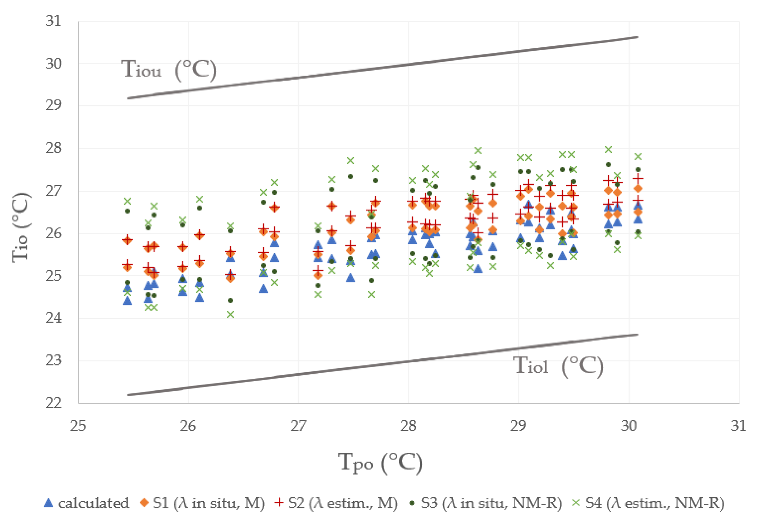
3.1.4. Indoor Operative Temperature (T_io)

The purpose is this subsection is to determine the correlation of the model through the indoor operative temperature. To do it, we are using the statements of the adaptative model described in the ASHRAE 55. As this method can only be used in free-floating conditions, the correlation of the computerised model with the actual building is only analysed during the month of July 2018. The T_io during this period has been calculated as the average value between the air temperature and the surface temperature of the wall.

This way, Figure 6 shows the in situ daily calculated maximum and minimum T_io values in the office and the daily simulated maximum and minimum T_io values. The T_io is represented depending on the prevailing outdoor temperature, which is an arithmetic mean as described in the methodology of this paper. The graph also displays the maximum and minimum comfort values for the T_io calculated through Equation (2) (T_iou) and Equation (3) (T_iol). Both the in situ calculated values and the results for the four simulations stay inside the comfort limits during the whole month, but we can see that for S1 and S2, when mass is considered, temperature is much more stable and similar to in situ calculated values.

3.2. Analysis of Simulated Comfort and Energy Demand

All four methods of correlation have demonstrated that the S1 alternative is the closest to the actual environmental behaviour of the room. Thus, in this section we will expose which of the four alternatives S1 to S4 shows better thermal comfort and energy demand performance.

3.2.1. Thermal Comfort

Figure 7 and Figure 8 show the results for the simulated T_io in the monitored room considering no heating (Figure 7) and no cooling (Figure 8), represented through boxplots.

During the winter period, as the prevailing outdoor temperature (T_po, calculated with Equation (4)) is always 10 °C, the minimum comfort operative temperature is T_iol = 17.4 °C (Equation (3)), and a line has been added to represent it. Here, although none of the simulations would show a compliance with the ASHRAE standard, we can distinguish that the results of S1 are closer to achieve it: the median, the mean and the minimum are the highest values of the four simulations. The difference between the minimum value and the T_iol is 3.02 °C, a difference of 0.87 °C with that obtained with S3 existing, more than 1.3 °C with S2 and more than 2.2 °C with S4. Also, there is more thermal stability in S1: 0.78 °C between the maximum and minimum temperature, while S2 is 0.96 °C, S3 is 1.13 °C and S4 is 1.41 °C. All this is detailed in

Table 9. Indoor operative temperature values in simulations (8–14 January 2018). No heating devices. In bold: values that would be closer to complying with ASHRAE 55.

Value	Mass		No Mass
	S1: λ in Situ	S2: λ Estim.	S3: λ in Situ	S4: λ Estim.
Maximum	15.16	14.03	14.64	13.57
Median	14.66	13.31	14.14	12.93
Mean	14.69	13.40	14.12	12.91
Minimum	14.38	13.07	13.51	12.14
Difference max—min	0.78	0.96	1.13	1.43
Difference minimum—Tiol	−3.02	−4.33	−3.89	−5.26

highlighting in bold values that would be closer to complying with ASHRAE 55.

For the summer period, T_iou and T_iol were already analysed in Figure 6, and we can see that all four simulations S1 to S4 and calculated values would comply with the ASHRAE 55. Figure 8 shows the boxplot for the one-week summer period (25–31 July), and as it happened in the winter period, we can also distinguish more thermal stability in S1, which would lead to a higher thermal comfort: there is a 0.77 °C difference between the maximum and minimum temperature, while this difference in S2 is 0.85 °C, in S3 is 2.15 °C, and in S4 is 2.74 °C.

3.2.2. Energy Demand

Figure 9 shows the energy demand of the studied room, obtained with DesignBuilder (called “Zone Sensible Heating/Cooling (kWh)” in this program), during the described periods of time described before (8–14 January and 25–31 July). Therefore, it gives us the idea of how much energy—in kWh/m²—requires the room to maintain the conditions described in Section 2.2.4 to achieve comfort during those periods of time. It is important to remember that heating and cooling systems use a time schedule “always on”.

A big difference can be distinguished when the λ-value is changed, as the S2 alternative requires 43% more energy in the winter week and 102% more energy in the summer week to keep the same comfort conditions as in S1. On the other hand, there is less difference when considering Mass and No Mass, as S3 only needs 7% more energy in the winter week and 53% more energy in the summer week than S1 to maintain comfort conditions. If we focus on the S4 alternative, it shows that it would require 45% more energy in the winter week and 131% more energy in the summer week to keep the same comfort conditions as in S1. Finally, if we extrapolate these results of the room to the whole year, the S1 would continue to be the alternative which requires less energy to keep optimum comfort. All this is shown in

Table 10. Energy demand (kWh/m²) of the room in S1–S4. % Difference between S1 and the rest of alternatives.

Period of Time	Mass			No Mass
	S1: λ in Situ	S2: λ Estim.		S3: λ In Situ		S4: λ Estim.
	kWh/m2	kWh/m2	dif.	kWh/m2	dif.	kWh/m2	dif.
8–14 January	5.38	7.72	+43%	5.74	+7%	7.81	+45%
25–31 July	−0.67	−1.37	+102%	−1.03	+53%	−1.56	+131%
Mean diff. weeks			+73%		+30%		+88%
Total heating year	90.61	128.95	+42%	96.07	+6%	137.28	+52%
Total cooling year	−5.13	−9.82	+91	−9.03	+76%	−13.83	+170%
Mean diff. year			+67%		+41%		+111%

.

4. Discussion

4.1. Validation of the S1 Alternative

The correlation between the four alternatives of the model S1–S4 and the actual room has been analysed using the R² parameter, through graphical comparison, determining the RMSE and the maximum temperature deviation, and using the adaptative model of the ASHRAE 55. The highest correlation occurs with the S1 version using any of the four methods, and therefore we have validated this simulation alternative as the one that would show reliable results, closer to the actual behaviour of the room.

While we have achieved a high R² correlation for the summer period between the air temperature in the model and the air temperature in the actual room, reaching a high correlation in Winter has been more difficult. This is because the studied room is in free-floating conditions during the summer, but in winter heaters were used. We studied activity information through surveys, but it was taken as general information during long periods of time and not describing in detail the activity for each day. Thus, in summer we get a high correlation between results regardless of the length of the period, but during winter we only get a high correlation when it comes to short periods of time (1 or 3 days) and lower correlation for periods of a week or longer.

This is also demonstrated when analysing the correlation through graphs and when determining the RMSE and the maximum deviation. In fact, differences between the measured dry-bulb temperature values and the results for S1 during the summer week are lower than the accuracy of the probes used to monitor the room (±0.3 °C). If we refer to the results for humidity, graphs show that the pattern of humidity inside the studied space is very similar, but there is a difference of 20% between actual and simulated values in winter (January) and 15% in summer (July). This is probably due to the chosen simulation method—CTF, or Conduction Transfer Function—which does not consider moisture storage nor diffusion of the walls.

It is important to remind that the influence of the thermal parameters would be lower in case we considered internal gains, but in any case, the studied building is a single-family dwelling with a low occupancy.

4.2. Influence of Estimated vs. Actual Properties of the Wall in Comfort and Energy Demand

Once having compared the S1–S4 alternatives with actual in situ values and having concluded that the S1 achieves a higher correlation, we have then used it to analyse comfort and energy demand, comparing the results of the four simulations to determine which alternative would generate a better performance.

We have determined the thermal comfort using the adaptative model described in the ASHRAE 55 for two weeks: 8–14 January and 25–31 July 2018. On the one hand, the indoor operative temperature (T_io) in S1 is more stable in both periods, which would therefore imply a higher thermal comfort. On the other hand, while all four simulations would reach comfort as per ASHRAE 55 during summer, none of them would in winter. This was already assumed and exposed in the introduction.

Nevertheless, the results of S1 are closer to achieve comfort. We can see this when we analyse the median and the mean values of the winter week, and because the difference between the minimum temperature value of the period is the closest to the lower 80% acceptability limit (T_iol) described in the ASHRAE 55 standard.

When we focus on energy demand, it has been demonstrated the importance of using measured values for the thermal conductivity. Using estimated values would result in 43% more energy in the winter week and 102% more energy in the summer week to keep the same comfort conditions as in S1. However, the calculation method used in the simulations (CTF) does not seem to consider the effect of thermal mass in the energy demand, as simulations 1 and 3, and 2 and 4 respectively, generate similar results, at least in the heating periods. Previous research stated that the CTF method is the best option in the climate where the building is located (BSk-Csa), but it did not reference the type of construction [38]. This may be a strong limitation on rammed earth walls, and the results in the previous paper [17] and other related research [48,49] show that the thermal conductivity value increases 7–10% for every 1% increase in water content.

Future research should include the effect of using different calculation methods such as HAMT (Heat And Moisture Transfer) or EMPD (Effective Moisture Penetration Depth), which consider moisture transfer, storage, and diffusion, for simulations that aim to estimate energy demand and consumption of buildings with high thermal inertia walls.

4.3. Influence of Estimated vs. Actual Properties of the Wall in the Compliance with the Spanish Code

Table 11. Compliance (in bold)/no compliance with the Spanish code: CTE DB HE 1. Simulations using CE3X software. In bold: values that would comply with the Spanish energy saving standard.

Condition		Limit (Zone D3)	S1: λ in Situ 1		S2: λ Estim. 1
			Value	Difference	Value	Difference
Energy demand 2 (kWh/m2 per year)	Heating	30.29 3	57.89	+91%	77.12	+155%
	Cooling	15.00 3	10.81	−28%	12.77	−15%
U (W/m2K)		0.41 5	0.65	+25%	1.35	+160%
K2,4 (W/m2K)		0.64 5	0.61	−5%	0.87	+36%

¹ Thickness of the walls = 0.63 m (mean value between thickness on the ground floor and thickness on the upper floor). ² Considering a U-value for glazing, roof, and ground slab that would comply with the code, which is usually reached in modern retrofitting. ³ As per CTE HE 1 2017 for new buildings. ⁴ Global heat transfer coefficient through the building’s envelope (K): mean heat transfer coefficient value for the heat exchange surface of the envelope. ⁵ As per CTE HE 1 2019 for restoration of buildings with a 25% envelope retrofitting.

shows the results obtained using the CE3X software, with the same conductivity values as per S1 and S2, and the compliance with the maximum values for energy demand, thermal transmittance of the walls (U in W/m²K) and global thermal transmittance of the whole building (K in W/m²K), described in the Spanish energy saving code. The limits considered in Table 11 are for the climatic zone D3, corresponding to the building location (these zones are described in Annex B of the code). Once the building has been modelled as described in the methodology section, we have verified the compliance with the code specifying the building as existent and supposing it would undertake a restoration of more than 25% of the envelope.

We have compared both the energy demand and the K-value considering that the glazing, roof, and ground slab would comply with the code, as the main problem of compliance with the code for existing traditional buildings is the U-value limit of the walls. Compliance with the U-value limit using standard values of conductivity for rammed earth walls leads to very thick insulations in these climate areas, underestimating the thermal capacity of the walls.

Again, the importance of using validated in situ measured values for the thermal conductivity is demonstrated when we are attempting to comply with standards like the Spanish energy saving code. Although both the thermal transmittance of the wall (U-value) and the heating energy demand of the building would exceed the limits described in the code, the requirement for the global thermal transmittance of the building (K-value) could be achieved without the need of adding thermal insulation. Moreover, the maximum U-value described in the code (0.41) could be reached with thinner insulations consisting in natural plaster based solutions: if we use a common exterior lightweight lime-cork insulating render with a thermal conductivity (λ-value) of 0.037 W/mK, the walls in S1 would require 3.5cm of insulation, while the walls in S2 would require 6.5 cm (a thickness difficult to achieve with a single-layer rendering).

Nevertheless, adding insulation would not be enough to comply with the heating energy demand requirements, but the new code has translated this requirement to consumption of non-renewable primary energy and consumption of total energy. Future research could be focused on the compliance of this requirement using a more detailed HVAC in simulations.

5. Conclusions

In summary, in this paper we have studied the influence of thermal parameters—conductivity, transmittance, and thermal mass—in the estimation of comfort and energy demand of a building with rammed earth walls, and consequently, the compliance of standards. To achieve it, we have used the results of a previous study that characterised those parameters of the wall [17], and we have monitored temperature and humidity in a room on the ground floor of the building, along with the outdoors dry-bulb temperature and relative humidity values to study the environmental conditions in the room and its surroundings during a whole year. We have then used all this information to analyse the correlation of four alternatives S1 to S4 of the same model in DesignBuilder through four different methods using temperature as the variable of comparison, as it was the parameter that was measured for the whole period and that affects both comfort and energy demand of the room. These methods are the R² coefficient of determination, graphical correlation, RMSE and the adaptative method of comfort described in the ASHRAE 55. The first three methods used the air temperature as variable, while this last method used the indoor operative temperature. The difference between the four versions of the model is that two of them use the in situ measured thermal conductivity (S1 and S3), and the other two use estimated values (S2 and S4), and on the other hand two of them consider thermal mass (S1 and S2) and the other two do not consider it (S3 and S4).

We have demonstrated through all four correlation methods that using actual parameters that describe the rammed earth wall will define a simulated model closer to reality (S1, in situ values).

When we analyse comfort in all four versions, we have showed that all of them would comply with the ASHRAE standard limits for indoor comfort using the adaptative model in summer, and none of them in winter, but the S1 version is closer to reach comfort in Winter: the difference between the minimum temperature value and the lower 80% acceptability limit (T_iol) is 3.02 °C, existing a difference of 0.87 °C with that obtained with S3, more than 1.3 °C with S2 and more than 2.2 °C with S4. Also, the S1 version achieves more stable indoor temperature conditions in both seasons as showed in the results section.

When we focus on energy demand, S3 would require 30% more energy, S2 would require 73% more energy, and S4 would require 88% more total energy to reach comfort than the S1 version. If we extrapolate the simulations to the whole year, we obtain similar results. When analysing energy demand, the fact that there is little difference between considering thermal mass (S1 and S2) and not considering it (S3 and S4) leads to the idea that the calculation method used in the simulations (CTF) did not take into account thermal inertia when evaluating energy demand.

Finally, once validated the more accurate and better performance of the S1 simulation alternative, when we consider the compliance with the Spanish energy saving code, we can assume that using these values in regulations compliance tools (like CE3X) would result in implementing much thinner retrofitting systems suitable for traditional buildings (i.e., exterior lightweight cork insulating renders): almost half the amount of insulation.

In conclusion, all these results show that using in situ measured parameters would lead to a better understanding of the behaviour of traditional rammed earth buildings, and thus ease their compliance with energy saving standards. This way, we try to encourage its use in new buildings, reducing the carbon footprint due to materials used in construction contributing to building construction that moves towards an ecological transition and sustainable development. Future research should analyse the impact in high thermal inertia buildings of using a different numerical method of simulations which consider important properties like moisture transfer, storage, and diffusion, such as HAMT (Heat And Moisture Transfer) or EMPD (Effective Moisture Penetration Depth). Also, future research should consider a more detailed HVAC to analyse the energy consumption of the different simulation alternatives.

References

1. IEA. Global Status Report for Buildings and Construction; Paris, France, 2019; Available online: https://www.iea.org/reports/global-status-report-for-buildings-and-construction-2019 (accessed on 7 December 2021).
2. IEA. Tracking Buildings 2020; Paris, France, 2020; Available online: https://www.iea.org/reports/tracking-buildings-2020 (accessed on 25 October 2021).
3. Giesekam, J.; Barrett, J.R.; Taylor, P. Construction sector views on low carbon building materials. Build. Res. Inf. 2016, 44, 423–444. [Google Scholar] [CrossRef]
4. IEA. Building Envelopes; Paris, France, 2019; Available online: https://www.iea.org/reports/building-envelopes (accessed on 7 December 2021).
5. CTE. DB HE: Código Técnico de la Edificación, Documento Básico de Ahorro de Energía (Spanish Energy Saving Code); Ministerio de Fomento: Madrid, Spain, 2019. [Google Scholar]
6. CTE. Código Técnico de la Edificación: Catálogo Informático de Elementos Constructivos (CEC). Available online: https://www.codigotecnico.org/Programas/CatalogoElementosConstructivos.html (accessed on 29 November 2021).
7. Baker, P. U-Values and Traditional Buildings in Situ Measurements and Their Comparisons to Calculated Values (Historic Scotland Technical Paper 10); 2011; Available online: https://www.historicenvironment.scot/archives-and-research/publications/publication/?publicationId=16d0f7f7-44c4-4670-a96b-a59400bcdc91 (accessed on 7 December 2021).
8. Rhee-Duverne, S.; Baker, P. Research into the Thermal Performance of Traditional Brick Walls (English Heritage Research Report); 2013; Available online: https://historicengland.org.uk/research/results/reports/70-2013 (accessed on 5 December 2021).
9. Asdrubali, F.; D’Alessandro, F.; Baldinelli, G.; Bianchi, F. Evaluating in situ thermal transmittance of green buildings masonries—A case study. Case Stud. Constr. Mater. 2014, 1, 53–59. [Google Scholar] [CrossRef]
10. Biddulph, P.; Gori, V.; Elwell, C.A.; Scott, C.; Rye, C.; Lowe, R.; Oreszczyn, T. Inferring the thermal resistance and effective thermal mass of a wall using frequent temperature and heat flux measurements. Energy Build. 2014, 78, 10–16. [Google Scholar] [CrossRef] [Green Version]
11. Li, F.G.N.; Smith, A.Z.P.; Biddulph, P.; Hamilton, I.G.; Lowe, R.; Mavrogianni, A.; Oikonomou, E.; Raslan, R.; Stamp, S.; Stone, A.; et al. Solid-wall U-values: Heat flux measurements compared with standard assumptions. Build. Res. Inf. 2015, 43, 238–252. [Google Scholar] [CrossRef] [Green Version]
12. Cuerda, E.; Romero, N.; Neila, F.J.; Guerra-Santin, O. Post-Occupancy Monitoring of Two Flats in Madrid: Development and Assessment of a Mixed Methods Methodology. In Proceedings of the PLEA 2015 Conference, Bolonia, Italia, 9–11 September 2015. [Google Scholar]
13. Ficco, G.; Iannetta, F.; Ianniello, E.; Alfano, F.R.D.; Dell’Isola, M. U-value in situ measurement for energy diagnosis of existing buildings. Energy Build. 2015, 104, 108–121. [Google Scholar] [CrossRef]
14. Marshall, A.; Fitton, R.; Swan, W.; Farmer, D.; Johnston, D.; Benjaber, M.; Ji, Y. Domestic building fabric performance: Closing the gap between the in situ measured and modelled performance. Energy Build. 2017, 150, 307–317. [Google Scholar] [CrossRef]
15. Lucchi, E. Thermal transmittance of historical brick masonries: A comparison among standard data, analytical calculation procedures, and in situ heat flow meter measurements. Energy Build. 2017, 134, 171–184. [Google Scholar] [CrossRef]
16. Balaguer, L.; Lopez-Manzanares, F.V.; Mileto, C.; Garcia-Soriano, L. Assessment of the Thermal Behaviour of Rammed Earth Walls in the Summer Period. Sustainability 2019, 11, 1924. [Google Scholar] [CrossRef] [Green Version]
17. Mascaraque, M.A.M.; Pacual, F.J.C.; Oteiza, I.; Secanellas, S.A. Hygrothermal assessment of a traditional earthen wall in a dry Mediterranean climate. Build. Res. Inf. 2020, 48, 632–644. [Google Scholar] [CrossRef]
18. ISO 9869-1. Thermal Insulation—Building Elements—In Situ Measurement of Thermal Resistance and Thermal Transmittance; International Organization for Standardization: Geneva, Switzerland, 2014.
19. Mellado Mascaraque, M.Á.; Castilla Pascual, F.J.; Oteiza, I.; Martín-Consuegra, F. In situ monitoring and characterisation of earthen envelopes: A review. In Proceedings of the SOSTierra 2017: International Conference on Vernacular Earthen Architecture, Conservation and Sustainability, Valencia, Spain, 14–16 September 2017. [Google Scholar]
20. Carrobe, A.; Rincon, L.; Martorell, I. Thermal Monitoring and Simulation of Earthen Buildings. A Review. Energies 2021, 14, 2080. [Google Scholar] [CrossRef]
21. Rincon, L.; Carrobe, A.; Medrano, M.; Sole, C.; Castell, A.; Martorell, I. Analysis of the Thermal Behavior of an Earthbag Building in Mediterranean Continental Climate: Monitoring and Simulation. Energies 2020, 13, 162. [Google Scholar] [CrossRef] [Green Version]
22. de Dear, R.J. Adaptative thermal comfort in building management and performance. In Proceedings of the Healthy Buildings: Creating a Healthy Indoor Environment for People, Lisbon, Portugal, 4–8 June 2006. [Google Scholar]
23. Heathcote, K. The thermal performance of earth buildings. Informes de la Construcción 2011, 63, 117–126. [Google Scholar] [CrossRef] [Green Version]
24. Serrano, S.; de Gracia, A.; Cabeza, L.F. Adaptation of rammed earth to modern construction systems: Comparative study of thermal behavior under summer conditions. Appl. Energy 2016, 175, 180–188. [Google Scholar] [CrossRef] [Green Version]
25. Olukoya Obafemi, A.P.; Kurt, S. Environmental impacts of adobe as a building material: The north cyprus traditional building case. Case Stud. Constr. Mater. 2016, 4, 32–41. [Google Scholar] [CrossRef] [Green Version]
26. Wati, E.; Meukam, P.; Damfeu, J.C. Modeling thermal performance of exterior walls retrofitted from insulation and modified laterite based bricks materials. Heat Mass Transf. 2017, 53, 3487–3499. [Google Scholar] [CrossRef]
27. Martin-Garin, A.; Millan-Garcia, J.A.; Teres-Zubiaga, J.; Oregi, X.; Rodriguez-Vidal, I.; Bairi, A. Improving Energy Performance of Historic Buildings through Hygrothermal Assessment of the Envelope. Buildings 2021, 11, 410. [Google Scholar] [CrossRef]
28. Lisitano, I.M.; Laggiard, D.; Fantucci, S.; Serra, V.; Fenoglio, E. Evaluating the Impact of Indoor Insulation on Historic Buildings: A Multilevel Approach Involving Heat and Moisture Simulations. Appl. Sci. Basel 2021, 11, 7944. [Google Scholar] [CrossRef]
29. Webb, A.L. Energy retrofits in historic and traditional buildings: A review of problems and methods. Renew. Sustain. Energy Rev. 2017, 77, 748–759. [Google Scholar] [CrossRef]
30. Hosseini, I.M.; Saradj, F.M.; Maddahi, S.M.; Ghobadian, V. Enhancing the facade efficiency of contemporary houses of Mashhad, using the lessons from traditional buildings. Int. J. Energy Environ. Eng. 2020, 11, 417–429. [Google Scholar] [CrossRef]
31. Mukhtar, M.; Ameyaw, B.; Yimen, N.; Zhang, Q.X.; Bamisile, O.; Adun, H.; Dagbasi, M. Building Retrofit and Energy Conservation/Efficiency Review: A Techno-Environ-Economic Assessment of Heat Pump System Retrofit in Housing Stock. Sustainability 2021, 13, 983. [Google Scholar] [CrossRef]
32. Parra-Saldivar, M.L.; Batty, W. Thermal behaviour of adobe constructions. Build. Environ. 2006, 41, 1892–1904. [Google Scholar] [CrossRef]
33. Avendano-Vera, C.; Martinez-Soto, A.; Marincioni, V. Determination of optimal thermal inertia of building materials for housing in different Chilean climate zones. Renew. Sustain. Energy Rev. 2020, 131, 110031. [Google Scholar] [CrossRef]
34. Kottek, M.; Grieser, J.; Beck, C.; Rudolf, B.; Rubel, F. World map of the Koppen-Geiger climate classification updated. Meteorol. Z. 2006, 15, 259–263. [Google Scholar] [CrossRef]
35. Sevilla, U.D. ENERGYTIC: Technology, Information and Communication Services for Engaging Social Housing Residents in Energy and Water Efficiency. Available online: https://grupo.us.es/grupotep130/es/proyectos/historico/506-energytic (accessed on 26 October 2021).
36. IETcc-CSIC. REFAVIV: Rehabilitación Energética De Las Fachadas De Viviendas Sociales Deterioradas En Madrid y Sevilla. Available online: https://proyectorefaviv.ietcc.csic.es/ (accessed on 26 October 2021).
37. Real Decreto 1027/2007, de 20 de julio, por el que se aprueba el Reglamento de Instalaciones Térmicas en los Edificios (RITE). 2021. Available online: https://www.boe.es/buscar/doc.php?id=BOE-A-2007-15820 (accessed on 5 December 2021).
38. Qin, M.; Yang, J. Evaluation of different thermal models in EnergyPlus for calculating moisture effects on building energy consumption in different climate conditions. Build. Simul. 2016, 9, 15–25. [Google Scholar] [CrossRef]
39. Houben, H.; Guillaud, H. Earth Construction: A Comprehensive Guide; Practical Action Publishing: London, UK, 1994. [Google Scholar]
40. Bauluz del Río, G.; Bárcena Barrios, P. Bases Para el Diseño y Construcción Con Tapial; Ministerio de Obras Públicas y Transportes: Madrid, Spain, 1992. [Google Scholar]
41. Minke, G. Building with Earth; Birkhäuser: Berlin, Germany, 2006. [Google Scholar]
42. Soebarto, V. Analysis of indoor performance of houses using rammed earth walls. In Proceedings of the Eleventh International IBPSA Conference, Glasgow, Scotland, 27–30 July 2009. [Google Scholar]
43. Mino-Rodriguez, I.; Naranjo-Mendoza, C.; Korolija, I. Thermal Assessment of Low-Cost Rural HousingA Case Study in the Ecuadorian Andes. Buildings 2016, 6, 36. [Google Scholar] [CrossRef] [Green Version]
44. Chel, A.; Tiwari, G.N. Thermal performance and embodied energy analysis of a passive house—Case study of vault roof mud-house in India. Appl. Energy 2009, 86, 1956–1969. [Google Scholar] [CrossRef]
45. ANSI/ASHRAE 55-2020. Thermal Environmental Conditions for Human Occupancy; American Society of Heating, Refrigerating and Air-Conditioning Engineers: Peachtree Corners, GA, USA, 2021.
46. Dong, X.; Soebarto, V.; Griffith, M. Achieving thermal comfort in naturally ventilated rammed earth houses. Build. Environ. 2014, 82, 588–598. [Google Scholar] [CrossRef]
47. Efinovatic. CE3X—Documento Reconocido Para la Certificación Energética de Edificios Existentes. Available online: http://www.efinova.es/CE3X (accessed on 28 October 2021).
48. Arnold, P.J. Thermal conductivity of masonry materials. J. Inst. Heat. Vent. Eng. 1969, 37, 101–108. [Google Scholar]
49. Chabriac, P.-A. Mesure du Comportement Hygrothermique du Pies; Université de Lyon: Lyon, France, 2014. [Google Scholar]
Figure 1. Studied building in Campo de Criptana (Ciudad Real, Spain): (a) North-facing façade in DesignBuilder, indicating the location of the monitored room (b) Panoramic view of the room.
Buildings 11 00635 g001
Figure 2. Plan view of the floors of the studied building in Campo de Criptana (Ciudad Real, Spain), indicating the monitored room with a red hatching.
Buildings 11 00635 g002
Figure 3. Internal and external temperature and relative humidity. 14 December 2017–15 December 2018.
Buildings 11 00635 g003
Figure 4. Indoor Air Temperature (Tia, °C). Measured values vs. simulations: (a) 8–14 January 2018 (b) 25–31 July 2018.
Buildings 11 00635 g004
Figure 5. Relative Humidity (RH, %). Measured values vs. simulations: (a) 8–14 January 2018 (b) 25–31 July 2018.
Buildings 11 00635 g005
Figure 6. Daily maximum and minimum indoor operative temperature (Tio) values depending on the prevailing outdoor temperature (July 2018). In situ calculated values and simulations.
Buildings 11 00635 g006
Figure 7. Indoor operative temperature values in simulations (8–14 January 2018). No heating devices.
Buildings 11 00635 g007
Figure 8. Indoor operative temperature values in simulations (25–31 July 2018). No cooling devices.
Buildings 11 00635 g008
Figure 9. Energy demand of the room due to heating and cooling. S1 to S4 during the selected weeks.
Buildings 11 00635 g009