1. Introduction
Tall-building wastewater drainage systems (WDSs) are comprised of wet stacks and networks of air vents. The function of these air vents is to allow wastewater to exit and induced airflow to enter efficiently and safely. Discharges subject the air within these systems to variable forces which initiate acoustic waves or pressure surges. The intensity of these surges generally depends upon the types of appliance being discharged; durations of discharges; the geometry of the appliance branches; the presence of pressure suppression components and, potentially, the condition of the sewer network. Prolonged surges which may result from the ‘heavy’ loading of a system (i.e., occurring as a result of extended-duration discharges) will generally result in the development of a dynamic suction pressure profile. Pressure surges may be large enough to delay or reverse sanitary water discharge; to initiate vibrations and cause noise; to deplete appliance trap seals by blow-out or siphonage [
1], or to deform or rupture pipework [
2].
The depletion of trap seals within the system is a particular concern. Empty trap seals provide a path for contaminated air to spread from the stack into the habitable space of a building. This spread is enhanced if local pressure in the stack is higher than the exterior pressure; under these conditions the stack actively expels contaminated air rather than removing it as intended. This ‘positive pressure’ has been shown to spread aerosolized pathogens [
3], and has been confirmed as the source of a SARS outbreak in Hong Kong [
4]. Coronaviruses are capable of surviving in sewerage systems for days to weeks [
5], and more recently, the SARS Cov-2 pathogen (‘COVID-19’) has been found in high concentrations in a WC in a hospital building [
6]. There is thus strong anecdotal evidence that the spread of COVID-19 is linked to malfunctioning WDSs; this has recently prompted risk assessments to have been carried out high-rise buildings [
7,
8]. These assessments indicate that risk is most substantial in the upper floors of high-rise buildings, and is non-negligible.
Steady progress has been made in recent decades in the identification, qualification and mitigation of pressure surges [
9]. However, this progress has largely been restricted to low-rise WDSs. Significant gaps remain in understanding of behaviour in high-rise WDSs [
10]. These gaps may be attributed the higher flowrates encountered in high-rise systems, greater network complexity, and the increased probability of interaction between discharges.
Operational problems are best avoided by
careful design, rather than by mitigation following construction. Building drainage system design codes have been developed with this goal in mind and are invaluable tools for building services engineers [
11,
12,
13,
14]. However, these design codes generally use ‘discharge unit techniques’ which apply a maximum water discharge rate (estimated by summing discharge units representing average flow of individual appliances) to recommend a stack size for a preferred configuration [
15]. The air supply configuration and the quantity of air entrained in the stack are not explicitly discussed within these design calculations. Hence, the design codes relegate a potentially very important aspect of WDS design, having potentially very significant impact for high-rise structures, to a position of triviality. This carries the risk that design might not be optimised, or, possibly, a novel design solution might be overlooked. It is these limitations which have prompt the development of a novel two-phase flow model which is described in this article.
1.1. Steady-State Pressure Profile
An important property of an operational drainage stack is its steady-state pressure profile. This is a hypothetical pressure profile which arises if it is assumed that the flows of water being discharged into the stack and associated rates of air intake remain perfectly steady over time. Note that, in the case of a high-rise building, these flows may be distributed (i.e., they may enter the stack at multiple locations). The profile provides a simple and convenient way to visualize the effectiveness of a design, since pressure extremes can easily be compared against a nominated design criterion, such as for example the 50 mm H2O pressure head typically provided by UK appliance water trap seals. This visualization is not possible when design codes are used to select a suitable design.
It should be noted that while a steady-state pressure profile provides useful design guidance, it does not on its own, guarantee an effective design. A drainage system will generally also require to be protected using active suppression components, or additional ventilation pipework in order to handle the larges surges which may occur if events cause air intake rates to change rapidly over time.
1.2. Modelling Software
The discussion above suggests the significant advantage to be gained through the development of a software tool capable of modelling the
two-phase (air-water) flow within in WDS networks.
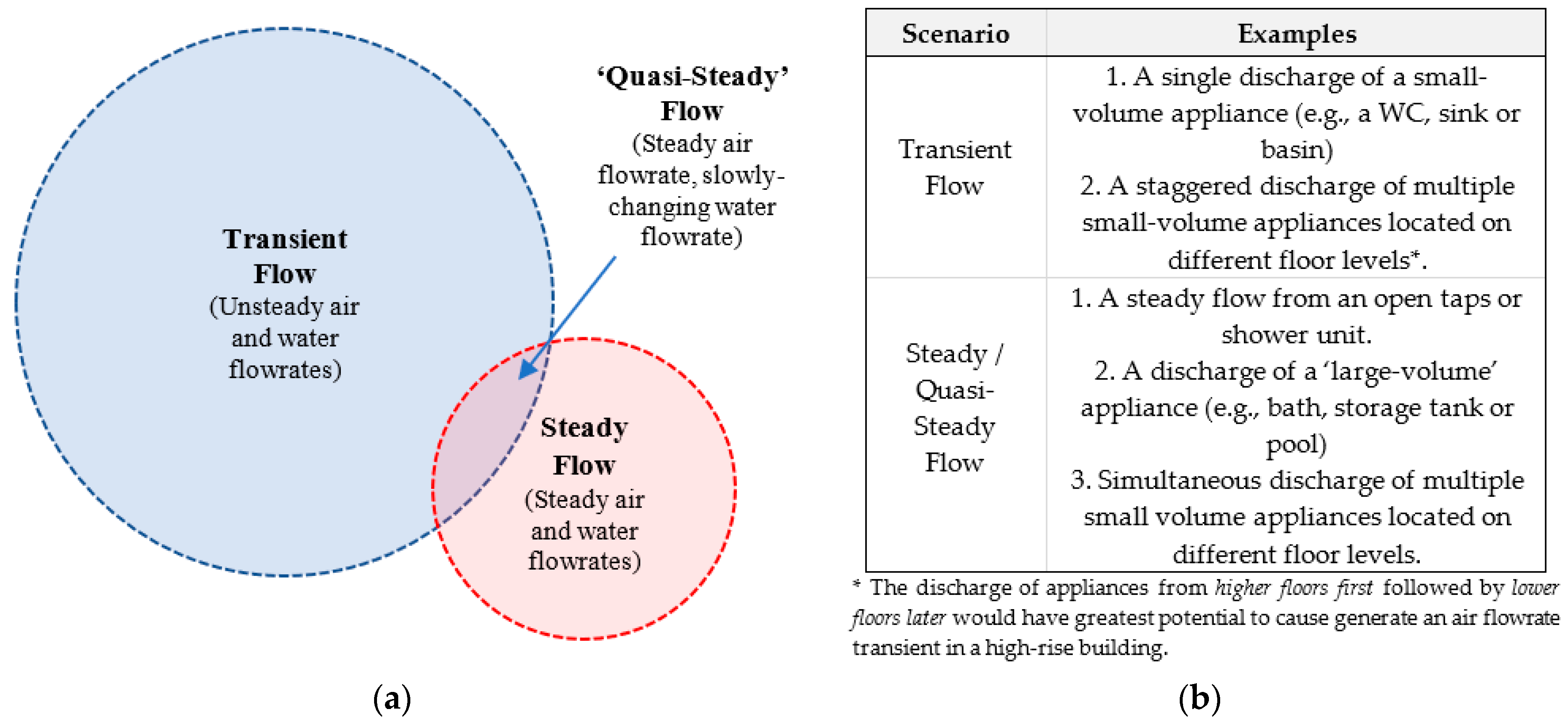
Figure 1a schematically illustrates the domain over which such a proposed tool would be required to function. The domain is divided into a
steady flow region, a
transient flow region, and an overlapping
quasi-steady flow region where, broadly speaking, the liquid flowrate changes sufficiently slowly over time as to resemble a steady flow. Examples of discharge events which would lead to these types of flows are suggested by the table to the right of the drawing. The transient flow region occupies a far larger space than the steady flow region, reflecting the greater number of ways in which wastewater can be discharged to produce unsteady flow and the greater likelihood that this unsteady flow can occur. However, it significant that from a practical viewpoint, steady flow is far easier to measure using an instrumented test rig and is also far simpler to model.
These observations motivate the development of a steady-state two-phase hydraulic model, for vertically downwards air-water flow. It is interesting to noted that similar types of tools have been developed for use within the nuclear power and the offshore oil and gas industries [
16,
17], and have now become integral to design procedures.
2. Background
Figure 2 illustrates a flow pattern map for fully developed air-water flow travelling at constant flowrates in vertical-downward pipes at atmospheric pressure [
18]. This map illustrates the tendency for fluids to arrange themselves into specific types of flow pattern, or flow geometries, depending upon the normalized flow velocities
and
. These normalized velocities are related to the volumetric flowrates
and
by:
Given sufficiently high values of water velocity
,
Figure 1 indicates that fluids will tend to flow in slug, bubble or churn patterns. In these patterns, the pipe core is either intermittently or permanently blocked by water. However, for lower values of water velocity
,
Figure 1 indicates that fluids will tend to flow in the annular pattern. In the annular flow pattern, liquid is pushed to the wall such that the core remains liquid-free.
Pressure gradients which arise due to bubble, slug and churn flow patterns are typically an
order of magnitude greater than pressure gradients arising due to an annular flow [
19,
20]. This observation implies that to minimize the potential for large pressure surges to occur in vertical drainage systems, the stack should be large enough to encourage the annular flow pattern and to discourage the bubble, churn or slug flow patterns as indicated by
Figure 1. The orientation of the transition boundary suggests that it easier to satisfy this requirement with a large, normalized air velocity U
a; that is to say, if a strong air current can be drawn through the vertical stack. A strong airflow is desirable as it permits a relatively small stack to be used; from an engineering perspective translates into savings in space and material costs.
2.1. Annular Flow Development
Water commingles with air at injection points, or junctions, in order to create air-water flowing mixtures. The experimental evidence suggests that local flow patterns in the vicinity of such junctions are strongly influenced by the junction geometry, but that these influences diminish with distance travelled downstream. Studies on vertical upwards annular flow suggest that pressure gradient and film volume fraction require around 100–300 diameters to develop from an inlet [
21], and that flow asymmetry reduces significantly with distance travelled downstream of U-bends [
22]. Studies on vertical downwards annular flow indicate sensitivity of flow development processes to inlet junction geometry [
23], and also to flow straightener devices which may be inserted to modify a flow profile [
24]. This evidence suggests that an annular flow develops downstream of an inlet, in a manner similar to a single-phase flow, and given a sufficiently long length of pipe, a
fully developed flow condition will establish. This fully developed flow condition will persist until an interruption such as a bend, a tee section, or a blockage, requires some level of
re-development to take place.
‘Fully developed’ annular flow is a quasi-steady condition, in that the phase fractions, phase velocities and pipe pressures are steady in an averaged sense but fluctuate on short timescales. The interface between the liquid annulus and the air core is poorly defined and highly turbulent (as compared to single-phase turbulent flow) and is periodically affected by instabilities such as ripples and roll waves [
25,
26]. Air in the core travels more rapidly than the water annulus, and as the boundaries with the churn flow and slug flow regimes are approached, the core absorbs water droplets which travel more rapidly than the air phase [
27]. The behaviour of annular flow remains incompletely understood. This means that uncertainty margins in two-phase annular flow models remain large, in comparison to single-phase flow models.
2.2. Steady-State Hydraulic Model Basis
Figure 3 shows an element of a developing annular flow within a drainage stack located at a distance
downstream from a discharging junction. The water within this element is subject to a body force
, a wall shear force d
and an interface shear force
, while the faces that the bound the element are subject to pressures
and
which are assumed to act uniformly across the element cross-section area. The differences in the face pressures cause net forces to acting upon the air phase,
, and the water phase,
, defined as:
where
is the pipe cross-section area (units m
2),
is the air phase cross-section volume fraction (dimensionless) and where Φ is the rate of change of pressure with distance
/
, i.e., the
axial pressure gradient (units N m
−3). For steady-state flow conditions, the force balance
+ d
+
+
0 applies.
The
overall pressure change between a junction located at
= 0 and a point located downstream distance
may be expressed as the sum of pressure contributions arising due to the junction and due to a developed annular flow. That is to say:
where:
and where
and
may be described as the
junction component and the
developed flow component of the pressure gradient
.
Two proposals are now made. Firstly, it is proposed that junction pressure gradient component
will tend asymptotically towards zero as the distance from the discharging
becomes large. That is to say, the net change in pressure which arises due to a junction has a finite value
which is defined by:
Secondly, it is proposed that the developed flow pressure gradient
is constant for any given set of normalized velocities
and
That is to say:
Equations (5) and (6) form the basis of a two-phase flow hydraulic model which can be applied to drainage stacks. And shall now be validated using the data which has been gathered from three experimental annular flow loops (‘test rigs’).
3. Experimental Apparatus
A significant amount of test data has been collected for gravity-driven annular downflow, using three different test rigs [
28,
29,
30]. These rigs (labelled A, B and C in the discussion below) may be represented schematically by
Figure 4a. Each rig comprises of an air inlet, a vertically downward-oriented test section hosting a water inlet, and an outlet. Each rig is instrumented with single-phase flowmeters, which record flowrates of air and water entering test sections, and with arrays of wall-mounted pressure transducers which record wall pressures within test sections.
A total of 107 tests have been conducted using Rigs ‘A’, ‘B’ and ‘C’ at the normalized velocities illustrated in
Figure 2 (these velocities lie left of the annular flow transition boundary, and are representative of operating conditions expected to be encountered within high-rise buildings). In each test, wall pressures are collected by pressure transducers for steady-state flow are averaged to produce basis data which is reproduced in
Section 4 and
Section 5. The three sets of basis data, comprised of 44 tests performed with Rig ‘A’, 27 tests with Rig ‘B’, and 36 with from Rig ‘C’, shall be referred to as the
basis datasets in discussions below.
Notable physical differences exist between Rigs ‘A’, ‘B’ and ‘C’ which are summarized by
Figure 4b. The test sections have different lengths, different diameters, and are made from different materials. The air flow is admitted either
actively (i.e., under pressure) or
passively (i.e., freely, without pressure). Rig ‘A’ is heavily corroded and discharges into a sewer, whilst Rig B and Rig C are made from smooth plastic materials and discharge into a collection tank. The locations at which water is injected into the test section vary between the test rigs, and the test sections are instrumented in different ways. In Rigs ‘A’ and ‘C’, pressure transducers are installed relatively far downstream of water inflow junctions, whereas in Rig ‘B’, pressure transducers are distributed through the test section downstream of the junctions.
The data generated from tests are now used to justify the proposals put forward in
Section 2.1 above and to derive empirical correlations for the
and
pressure gradient components shown in Equation (4). It is to be noted that these correlations apply only to steady flow in straight pipe sections, bounded by the conditions shown in
Figure 2. Nevertheless, these correlations are sufficiently robust to permit the analysis of drainage networks as is to be described in
Section 6.
4. ‘Junction’ Pressure Gradient Component
Figure 5a illustrates mean wall pressures which are obtained from the Rig ‘B’ basis dataset (comprised of the 24 sets of data obtained for conditions shown in
Figure 2, at elevations shown in
Figure 3). The data are displayed in the form of pressure change relative to the wall pressure above discharging junctions,
, versus normalized distances from junctions
. (The data obtained from the transducer located at the base of the stack, just above the 90° base elbow, are omitted).
The data shown in
Figure 4a are interpreted more easily by superimposing trend lines which take the form:
where
is the developed flow pressure gradient component (defined in Equation (4) and evaluated using the techniques described in
Section 5 below) and where
and
are empirical constants. The values of
and
are obtained from the data using the methods summarized in
Table 1. These trendlines highlight that the pressure gradients increase monotonously with distance and tend towards limiting values as was proposed in
Section 2.1 above.
Figure 5b illustrates the residual pressure gradient component
which is derived by evaluating the quantity
and corresponding trendlines
which may be derived from Equation (7). These data suggest that the
component tends asymptotically toward limiting values which are defined by Equation (5) and which are strongly dependent upon the water velocity
.
Empirical Correlation
An empirical correlation for the gradient
is developed as follows. The gradient
is assumed to be the product of a net junction loss parameter,
, and a distance-dependent decay parameter γ according to the expression:
These parameters
and γ are related to the parameters
and
, used to fit trend lines as described in
Table 1, as follows:
Figure 6 and
Figure 7 display values for
and
as a function of normalized velocities
and
. The parameter
is strongly dependent upon
but weakly dependent upon
. The data suggest an empirical correlation for parameter
may be developed which takes the form:
where the coefficient values
= −390 mm H
2O/ms
−1 and b
2 = 33 mm H
2O provide the fit to the data shown in
Figure 6b. The constraint
= 0 is imposed for
< 0.085 ms
−1, implying that there is no junction pressure gradient component for sufficiently low discharge water velocities.
The parameter k
2 on the other hand appears to be strongly dependent on
but rather weakly dependent on U
w. For simplicity, the average value:
is assumed such that the single curve illustrated in
Figure 7b defines the behavior of the junction pressure component
. This single parameter value provides a reasonable fit to all data.
Equations (8)–(11) are, of course, applicable for the one specific type of discharge junction installed within Rig ‘B’ spanning the range of normalized velocities shown within
Figure 2. Comparison with Rig ‘A’ and Rig ‘C’ is not possible (Rigs ‘A’ and ‘C’ lack suitably located pressure transducers to enable such comparison to be made). However, experimental evidence suggests that junction losses are sensitive to the branch line diameter and angle of discharge from the branch line into the stack [
31].
5. ‘Developed Flow’ Pressure Gradient Component
Figure 8 illustrates developed flow pressure gradient components
which may be derived from the Rig ‘A’, Rig ‘B’ and Rig ‘C’ datasets using data from transducers located downstream of junctions. The
values are plotted as a function of the air velocity U
a and trend lines indicate constant values of velocity
. Each
value is derived from the expression:
where
and
are the pressure data obtained from the pressure transducers furthest downstream of junctions having separation distance
. Note that the caveats shown in
Table 2 are applied during calculation (which mean that strictly speaking, the data derived from Rigs ‘A’ and ‘C’ are estimates of
).
The spread of data in
Figure 8 reflects the significant physical differences between Rigs ‘A’, ‘B’ and ‘C’ that are summarized in
Figure 4b. However, the
estimates are always positive for low
values (i.e., pressure increases as vertical elevation decreases), and for these positive values, the trend lines indicate that:
The derivative is negative, i.e., pressure gradient Φd decreases with increasing air velocity.
The derivative is positive, i.e., pressure gradient Φd increase with increasing water velocity.
The derivative is negative, i.e., rate of change of gradient decreases with increasing water velocity.
All three sets of data display these trends, suggesting that they might be universal trends for vertical-downwards, gravity-driven annular flow.
5.1. Empirical Correlation
Three empirical correlations for
are developed, on the basis that there are significant differences in flowrate conditions tested using Rigs ‘A’, ‘B’, and ‘C’. Each empirical correlations is developed by assuming that
is a function of velocities
and
defined by the polynomial
:
where polynomial coefficients
to
are obtained by least-squares regression techniques, with exponent values i = j = 1 are applied as ‘base case’. The appropriate coefficient values
,
and
for Rigs ‘A’, ‘B’ and ‘C’ are summarized in
Table 3, while
Figure 9a–c display the resultant functions
,
and
. (These figures also show that by adjusting exponent values i = j = 1.5, extrapolation behavior the available range of data can be controlled).
Figure 9d illustrates
differences between functions
and
, for the limited regions of overlap between datasets shown in
Figure 2 where this comparison is applicable. The difference
is small, implying that Rigs ‘A’ and Rigs ‘C’ produce similar results. The difference
is larger, indicating there is higher (positive) pressure gradient derived from Rig ‘B’ data. These differences reflect differences in annular film thickness, wall friction forces and interface friction forces between the test rigs, as well as possible pressure losses due to the stack geometry.
5.2. Limiting Air Velocity
A notable difference between the datasets plotted in
Figure 8 is that the calculated
values are consistently positive for Rigs ‘A’ and ‘B’, whereas calculated
values eventually become
negative as
is increased for Rig ‘C’. This difference arises as the air feeds in Rigs ‘A’ and ‘B’ is
passive, whereas the air feed in Rig ‘C’ is
active (that is to say, the air feed may be compressed such that it is drawn in at elevated pressure rather than atmospheric pressure). As Rig ‘C’ ejects air to atmosphere, this compression can support negative pressure gradients within the test section.
The air velocities at which the
values cross zero may be defined as
limiting velocities (
. The data in
Figure 6 suggest that the junction component
is consistently negative, and therefore, the
and
values will have opposing polarity on the condition that
. This opposing polarity ensures the downwards flow of air through the test sections. Moreover, this opposing polarity implies that the maximum air velocity which may be drawn through a
naturally ventilated drainage stack
is , which applies regardless of stack height. This limit cannot be exceeded without performing work on the inflowing air stream.
Figure 10 illustrates ‘limit velocity functions’
(U
w) that are derived using the correlation coefficients listed in
Table 3 (Rigs ‘A’ and ‘B’ these functions require data shown in
Figure 9a,b to be extrapolated, to develop these functions for Rigs ‘A’ and ‘B’. Therefore, the values shown in
Figure 10 are estimate values for
and they are displayed for a much smaller span of
values than Rig ‘C’). The functions take quadratic forms, reflecting the fact that the data in shown in
Figure 9 have been nominally fitted using a cubic polynomial. Despite the physical differences between the three test rigs, the
functions shown are very similar. The functions tend toward a plateau value of the order of 6 ms
−1 as
is increased, suggesting that a maximum air velocity limit velocity of the order of 6 ms
−1 applies to all naturally ventilated vertical drainage systems. A similar tendency for the water velocity to plateau in this may be observed by analyzing data for large-diameter plunging dropshafts [
32].
6. Network Analysis
Equations (8)–(11) and (13) can be employed to examine steady-state pressure profiles in a wastewater system network, such as the example system which is shown in
Figure 11. This system is comprised of seven branches and seven nodes, with the wet stack accepting discharge water at nodes B and C (at velocities
and
), and drawing in air from roof nodes A and B (at velocities
and
. The boundary nodes A, D and E are open to atmosphere, while the vent line is permitted to exchange air with the wet stack via two crossover valves (XOVs). For design purposes the water velocities
and
may be treated as the system inputs while the air velocities
and
may be treated as unknowns.
The air velocities in branches, the hydraulic pressures at nodes, and the hydraulic pressure profiles between nodes shown in
Figure 11 can be derived, provided that pressure gradients for flow in the dry branches (
) and the wet branches (
) are supplied. If, for simplicity, the lengths of the crossover lines FB and CD are assumed to be zero, these parameters are obtained by solution of:
where
,
,
,
and
are the pressure losses across the branches. Equation (14) may alternatively be expressed as:
where
,
,
,
and
are the lengths of the branches shown in
Figure 9. The single-phase (air) pressure gradients
may be derived from the classical expression:
using an appropriate expression for the Darcy friction factor
. The two-phase pressure gradients Φ are evaluated Equations (8)–(11) and (13).
Two assumptions are now introduced in order to handle merging of fluids with the two-phase stream, as the discharge travels from branch BC to branch BD. The first assumption is that if the merging fluid is water, the junction pressure gradient component associated with this fluid is a function of the combined water flow velocity. Referring to node C within
Figure 11, that is to say:
The second assumption is that if merging fluid is air, there is no junction pressure gradient component; i.e., there is no penalty associated with the air intake. Again, referring to node C in
Figure 11, that is to say:
Equations (17) and (18) close the hydraulic model, such that the drainage network shown by
Figure 11 may be analyzed.
7. Preliminary Case Study
Solutions for a preliminary case study are now presented, based on the nominated parameter values shown in the table to the right of
Figure 11 (i.e., a 40-m 4-in ID stack with a 3-in ID vent line, subject to ‘single junction’ and ‘dual junction’ discharges through nodes B and C). For this analysis the pressure gradient parameter
is evaluated using the
function coefficients listed in
Table 3 while the pressure drop across the air admittance value (AAV) is evaluated from the expression:
where the loss coefficient, K, has a nominated value of 100 as suggested by experimental testing [
33].
Figure 12 illustrates air velocities in the network branches and pressure profiles though the stack for the two sets of simulation cases. The tables indicate that air flow through the network increases as the total water discharge rate increases and as the XOVs are opened. The air velocities approach, but do not exceed, the limiting values
defined in
Figure 7 when both XOVs are open (i.e., air supply configuration (d)). The graphs indicate that the suction pressures are most extreme when water is discharged through both nodes and when both XOVs are closed (minimum −87 mm H
2O for the dual-discharge scenario with air supply configuration (a); with a notable contribution across the AAV). By opening the XOVs alleviates the suction pressures throughout the entire wet stack are alleviated.


