Abstract
Deep learning technology, such as fully convolutional networks (FCNs), have shown competitive performance in the automatic extraction of buildings from high-resolution aerial images (HRAIs). However, there are problems of over-segmentation and internal cavity in traditional FCNs used for building extraction. To address these issues, this paper proposes a new building graph convolutional network (BGC-Net), which optimizes the segmentation results by introducing the graph convolutional network (GCN). The core of BGC-Net includes two major modules. One is an atrous attention pyramid (AAP) module, obtained by fusing the attention mechanism and atrous convolution, which improves the performance of the model in extracting multi-scale buildings through multi-scale feature fusion; the other is a dual graph convolutional (DGN) module, the build of which is based on GCN, which improves the segmentation accuracy of object edges by adding long-range contextual information. The performance of BGC-Net is tested on two high spatial resolution datasets (Wuhan University building dataset and a Chinese typical city building dataset) and compared with several state-of-the-art networks. Experimental results demonstrate that the proposed method outperforms several state-of-the-art approaches (FCN8s, DANet, SegNet, U-Net, ARC-Net, BAR-Net) in both visual interpretation and quantitative evaluations. The BGC-Net proposed in this paper has better results when extracting the completeness of buildings, including boundary segmentation accuracy, and shows great potential in high-precision remote sensing mapping applications.
1. Introduction
Automatic building extraction from remote sensing images (RSIs) has been a hot topic in the field of photogrammetry and remote sensing for decades [1,2]. The end product is extremely important for various applications, such as mapping, spatial planning and urbanization processes [3,4,5,6]. With the continuous advancement of remote sensing technology, the imaging quality and spatial resolution of RSI have been improved. Among them, high-resolution aerial images (HRAIs) have become the preferred data source for building extraction due to their rich feature information and texture semantics. However, the increase of redundant interference information in HRAIs and the highly complex urban scenes bring difficulties and challenges to the high accuracy extraction of buildings.
Traditional methods for building extraction from RSIs mainly include pixel-based methods and object-oriented methods [7,8]. The pixel-based method is based on a single pixel as the processing object, and extract the building by obtaining its spectrum, shape, and geometric features [9,10,11]. This method is easy to implement, but it generates more noise and is less effective in complex scenes. The object-oriented method is generally based on image segmentation, with feature patches as the smallest unit of analysis, and is a method of segmentation before classification. Du et al. [12] designed linearization and global regularization algorithms to draw residential contours from large-scale point clouds for building extraction. Awrangjeb et al. [13] combined LIDAR data and aerial imagery to effectively improve building extraction accuracy. Cui et al. [14] used a minimum spanning tree with a rectangular index to control the segmentation scale, which extracted a better building integrity. Li et al. [15] used worldview-2 data for a better extraction of buildings through an object-oriented method, but the segmentation scale and rules of the method are more complicated to determine. Li et al. [16] firstly used a multi-scale segmentation method to divide the image objects, and then established a classification system and function rules to extract residential buildings, which effectively solved the problem of “same objects with different spectra”. Yan et al. [17] implemented object-oriented detection of building damage information based on a multi-classifier system. However, the object-oriented methods require artificially selected classification rules, which not only have the problems of large workload and low efficiency, but also poor generalization ability of multi-source information extraction. Therefore, there is an urgent requirement for a more effective and intelligent means of building extraction from RSIs.
In recent years, the rapid growth of computational power has facilitated the development of deep learning, especially convolutional neural networks (CNNs), which has become a powerful tool for image processing [18]. CNNs can not only automatically extract features from raw image data, but also obtain semantic information level by level, which has achieved great success in image classification tasks [19,20,21] and provides a new solution for building refinement extraction. In 2015, Long et al. [22] proposed a fully convolutional network (FCN), the first end-to-end semantic segmentation method implemented in neural networks. Following this paradigm, many scholars have further considered the relationship between inter-pixel space and values, while many deepened and improved networks are proposed, such as U-Net [23], SegNet [24], DeconvNet [25], etc. However, these networks lose some detail information while obtaining multi-scale features, they are not the best solution for addressing the task of building segmentation [26].
In order to obtain the multi-scale features of buildings more effectively, researchers have proposed some new networks based on FCN. Jin et al. [27] designed the DASPP module based on DeepLabv3+ to solve the problem of missing boundary information, and proposed BARNet to extract buildings in complex urban scenes with high accuracy. Pan et al. [28] proposed a new network DPN, which first processes the sensor data using group convolution to obtain the feature maps of individual channels, and then goes through the pyramid module to fully acquire the high-level features. Liu et al. [29] designed a deep encoder–decoder network. The network uses striding convolution to obtain information at multiple scales during down-sampling, while using densely upsampling convolution to recover feature map dimensions. The effectiveness of this network was verified on the WHU dataset and the SuZhou dataset. To integrate the semantic information of buildings of different sizes, SR-FCN [30] adds atrous spatial pyramid pooling (ASPP) to the decoder. AWNet [31] proposed an Adaptive Multi-Scale Module, which can adaptively fuse features according to the change of building feature size. MAP-Net [32] uses a multi-parallel strategy to obtain multi-scale building footprint features, followed by feature fusion using an attention mechanism. Sun et al. [33] first extracted deep features at different scales using multi-scale CNN, then input them into a different support vector mechanism (SVM) for feature processing, respectively, finally refining the boundary to output the segmentation results. This method can achieve high precision extraction of building contours in urban scenes. However, the above methods do not add global dependencies when capturing local features, and lack guidance from long-range contexts, which can easily cause the loss of building feature information. At the same time, due to the complexity of the scenes in HRAIs, there are still many difficulties for existing networks to make a high-precision segmentation of buildings [34,35,36].
Based on the above analysis and discussion, we have designed two modules to solve the above problems. To address the problem that existing networks cannot make good use of multi-scale features, we propose the atrous attention pyramid (AAP) module. Based on the classical pyramid feature extraction structure, a new branch feature fusion method is proposed, and a spatial attention mechanism is added to deepen the semantic information of each branch. To make more efficient use of long-range contextual information, we construct a dual graph convolution (DGC) module to model global dependencies.
The main contributions of this work are summarized as follows:
- (1)
- A new multi-scale feature fusion module, the AAP (atrous attention pyramid) module, is proposed to fuse multi-scale features through the combination of multi-branching and attention mechanisms, which helps network to cope with complex scenes with variable building dimensions.
- (2)
- The DGC (dual graph convolution) module is used to obtain global contextual information in spatial and channel dimensions. This module guides the network to perceive effective features from the global context, reduces the influence of the background environment on building recognition, and allows more accurate identification of the classes to which edge pixels belong.
- (3)
- A new network, the building graph convolutional network (BGC-Net), is proposed. The proposed method was thoroughly evaluated on two different and versatile datasets, which confirmed that the proposed method can comprehensively outperform the existing CNN-based methods in the Overall Accuracy (OA), Recall, F1 score, and intersection over union (IoU).
2. Methodology
2.1. Overview of the Proposed Model
In this paper, we propose a combined FCN and GCN model named BGC-Net; the overall structure is shown in Figure 1. BGC-Net is designed as an asymmetric encoder–decoder structure, consisting of three modules: a feature extraction (FE) module, atrous attention pyramid (AAP) module, and dual graph convolutional (DGC) module. The input HRAIs are first processed by the FE module to capture the building feature information at different levels. The obtained high-level building features are input to the AAP module, which constructs a pyramid based on the atrous convolution and attention mechanism to effectively capture the global dependencies and contextual information for a better feature representation. Finally, in order to improve the pixel-level prediction accuracy of the buildings, the interdependencies between the channel feature maps as well as the pixel feature maps are modeled using the DGC module.
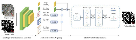
Figure 1.
The structure of our proposed BGC-Net, consisting of three parts: FE module, AAP module, DGC module.
2.2. Feature Extraction Module
The input HRAIs are first processed by the FE module to capture the building feature information at different levels. To improve the feature extraction accuracy, some networks, such as VGG and AlexNet, obtain better training results by increasing the network depth. However, the increase of network depth brings gradient explosion and gradient vanishing phenomenon, which affects the training and prediction of the network. To address this issue, ResNet [37] was proposed with the direct mapping between deep and shallow neurons. The skip-connection integrates the original information with the high-level semantics, effectively preventing the gradient from vanishing during backpropagation. The structure of the residual block is shown in Figure 2. For ResNet, when the number of network layers is enough, the network has already reached the maximum feature extraction capacity and increasing the network depth again does not improve the feature extraction effect much. Based on this, after an experimental comparison analysis and comprehensive consideration of model accuracy and efficiency, we finally choose ResNet-50 to constitute the FE module of BGC-Net; its structure is shown in Figure 3.
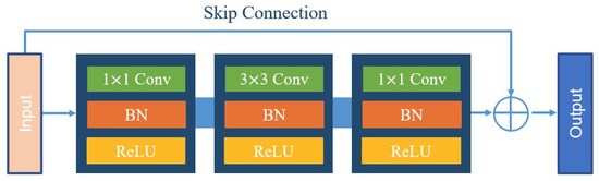
Figure 2.
The structure of the residual block.
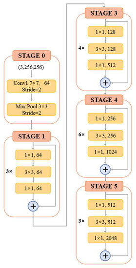
Figure 3.
The structure of ResNet-50.
ResNet-50 consists of five stages. The first stage consists of a 7 × 7 convolution and a max-pooling layer for the down-sampling operation of the input image. Each of the four subsequent stages consists of a different number of residual blocks. The residual block contains two 1 × 1 convolutional and one 3 × 3 convolutional constructs, while fusing low-level and high-level features by skip-connection. Subsequently, the features are processed using the rectified linear unit (ReLU) function as well as the batch normalization (BN) layer, thus ensuring a uniform distribution of the features in each layer. Finally, the obtained feature maps are used as an input to the AAP module, which is used for further contextual information extraction.
2.3. Atrous Attention Pyramid Module
For the problem of difficult classification caused by the existence of multi-scale buildings in HRAIs, the AAP module is proposed in this paper. The AAP module captures multi-scale features by aggregating atrous convolutions and uses a spatial attention mechanism to make each layer more focused on building features, which helps to enhance the prediction capability of targets at different scales.
Through constructing different branches to extract features separately, and finally fusing different samples, the pyramid structure is considered as an effective way to extract multi-scale features [6,38]. Zhao et al. [39] proposed a pyramid pooling module to aggregate contexts at multiple scales, which enhanced the scene parsing capability of the network and improved the accuracy of image segmentation results. Chen et al. [40] combined different rates of atrous convolution and image-pooling to construct ASPP that obtains multi-scale association information. Yang et al. [41] proposed a densely connected ASPP, which organizes different rates of atrous convolution layers in a cascade fashion. The output features of each layer are fused with the input features, and together they are used as feature inputs for the next layer. The final output of each branch integrates all the information from the previous layers, thus obtaining multi-scale information with better results.
The attention mechanism can focus on regions of interest to optimize the feature extraction process, which is widely used in the image field [42]. Among them, the spatial attention mechanism (SAM) gives more attention to locally important information by weighting the feature map, which promotes the classification accuracy among different local features [43]. The SAM structure is shown in the bottom half of Figure 4. The input feature map is first transposed and then multiplied with the feature map matrix to obtain the attention map S. Then S is matrix multiplied with the transpose of the feature map to obtain the feature map of each position weight. Finally, this map is added with the original feature graph to obtain the final output of the integrated correlation results.
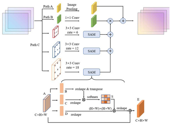
Figure 4.
Structure of atrous attention pyramid module in the BGC-Net.
The AAP module proposed in this paper is shown in Figure 4. This module includes image-pooling, 1 × 1 convolution, and three branches of atrous convolution containing a SAM. In order to better extract contextual information from different scales, the rate in the atrous convolution of the AAP module is set to 6, 12 and 18, respectively. Meanwhile, the SAM is added in each branch to improve the feature extraction for buildings at different scales. The pyramid gradually integrates information at different scales according to the RF size, making full use of the hierarchical dependence of contextual information, and then multiplies the fusion results with the feature map after 1 × 1 convolution. Finally, the AAP module in this paper introduces the image-pooling layer to obtain global high-dimensional features. It is used to further reduce the loss of features and to obtain more effective multi-scale information.
2.4. Dual Graph Convolutional Module
Adding long-range contextual information to the CNN enables the network to extract more complete semantics, which enhances the network’s ability to parse scenes [44]. Therefore, in this paper, the DGC module is designed to model the contextual information of the input features in spatial and channel dimensions. This enhances the feature learning of building area pixels and enables better building feature extraction.
In HRAIs, the spatial distribution between different types of features is strongly correlated. However, traditional deep semantic segmentation networks have difficulty in handling this spatial topological relationship information, which is extremely important for image interpretation [45]. Graph convolutional network (GCN), as an application of deep learning on graph data, has obvious advantages in processing these non-Euclidean spaces [46,47]. Based on this, inspired by several works [48,49], this paper develops the DGC module based on GCNs. The DGC module can better distinguish different objects by detecting features from the global, thus improving segmentation accuracy.
The structure diagram of the DGC module is shown in Figure 5, which is divided into two parts: spatial dimension GCN and channel dimension GCN. The main purpose of the spatial dimension GCN part is to explicitly model the spatial relationships between individual pixels in the image, obtaining correlation predictions considering all pixels. First project the input feature into the coordinate space , and transform it into the new feature in using the spatial down-sampling operation. where represents the feature dimension, and represents the number of nodes of the feature.
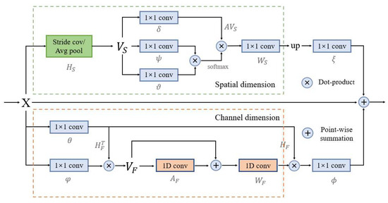
Figure 5.
Structure of the dual graph convolutional module in the BGC-Net. This module consists of two branches, which each consist of a graph convolutional network (GCN) to model contextual information in the spatial- and channel-dimensions in a convolutional feature map, X.
The new feature is defined as follows:
where denotes the sampling rate of spatial down-sampling, and represents the spatial down-sampling.
On this basis, a lightweight fully connected graph is constructed, which is used for information dissemination across nodes. Global relational inference for the new feature has three linear variations and is used to model the relationships that exist between the nodes. Obtain the new feature :
where ,, are the three linear transformations and is the weight matrix.
Finally, it is inverse mapped into the original space, and resized using the nearest neighbor interpolation method:
where is the inverse mapped posterior feature and is the closest interpolation method.
The main purpose of the channel dimension GCN part is to model the interdependence between the channel dimensions of the network feature mapping, which can obtain more abstract feature information in the image. First, the input feature is projected onto the feature space to obtain the new feature :
where is used to reduce the channel dimension of , and is the projection function, and are linear transformations.
Then, build the lightweight fully connected graph containing the adjacency matrix, such that each node in the graph contains the symbols describing the features. Obtain the feature :
where is the edge weight and is the unit matrix.
On this basis, the feature is obtained by mapping into the original coordinate space. Finally, the output feature .
2.5. Decoder Module
The main task of the decoder phase is to up-sample the feature maps and to recover the input resolution from the encoder phase. Inspired by the idea of a light-weight and asymmetric decoder, we designed a simple and effective decoder module. The proposed decoder module is shown in Figure 6. The feature maps obtained by the FE module, AAP module and DGC module are fused, in turn, to obtain a new feature map containing high- and low-level semantic information. Further, the feature map is output as a binary map with a channel number of 1 by upsampling to enlarge the size of the fused feature map and reducing the channel number.
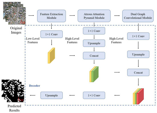
Figure 6.
Structure of the decoder module in the BGC-Net.
3. Experimental Datasets and Evaluation
3.1. Datasets
In this study, the WHU building dataset (WHU dataset) [50] and the China typical city building dataset (CHN dataset) [51] were used to verify the performance of the proposed network. The two datasets are taken from complex urban scenes in different regions with very high resolution. The basic parameters and image examples are shown in Table 1 and Figure 7.

Table 1.
Basic parameters and training assignment of dataset.
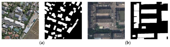
Figure 7.
Examples of the images and corresponding labels for the two employed datasets. (a,b) represent the WHU dataset and CHN dataset, respectively. The white pixels stand for buildings.
WHU building dataset: Provided by Prof. Shunping Ji’s team at Wuhan University, it is a building detection dataset based on large-scene, high-resolution RSIs. The dataset mainly covers part of Christchurch, New Zealand, with an overall coverage area of 450 km2. The whole image is divided into 3 bands of RGB. The dataset contains a total sample of 22,000 buildings of different styles, functions, sizes, and colors. The WHU dataset surpasses the current international mainstream building dataset in several metrics such as size, resolution, and accuracy.
Chinese typical city building dataset: The images were taken from four representative urban centers in Beijing, Shanghai, Shenzhen and Wuhan, covering an area of 120 km2. The dataset contains orthophotos, non-orthophotos, sparse distribution of buildings and dense distribution images, containing 63,886 buildings. It is a more challenging dataset with richer imaging angles and building classes than the WHU dataset.
In order to avoid overfitting during network training due to the small training sample size, the training set images are processed by data enhancement, including image rotation and random flip.
3.2. Evaluation Metrics
In order to evaluate the performance of the network more comprehensively, Overall Accuracy (OA), Precision, Recall, F1-score and Intersection-over-Union (IoU) are chosen as evaluation metrics. The evaluation indicators are calculated as follows:
where TP is the true positive, TN is the true negative, FP is the false positive, and FN is the true negative. OA indicates the percentage of correct predictions among all pixels. Precision is the number of pixels correctly predicted as a positive class divided by the number of pixels predicted as a positive class. Recall is the number of pixels correctly predicted to be in the positive class divided by the number of pixels in all positive classes. The F1-score takes into account both Precision and Recall. IoU can describe segment-level accuracy.
3.3. Implementation Details
In this paper, in order to verify the building extraction performance of BGC-Net, the current better performance and widely used U-Net, SegNet, DANet, and FCN8s are introduced as comparison methods. The five networks were tested on two datasets, using the same training set, validation set and test set, and the same software and hardware environment for training. The software and hardware configurations for this experiment are shown in Table 2. The same parameter settings were performed for all networks: the Adam optimizer [52] was selected and the initial learning rate was set to 0.0001, = 0.9, and = 0.999. The network has a batch size of 4 and a learning rate of 0.001, with 150 epochs trained on each of the two datasets.
Table 2.
Hardware and software configuration.
4. Results
4.1. Visualization Results
4.1.1. Results on WHU Dataset
The results of the building segmentation for different networks on the WHU dataset are shown in Figure 8. From an overall perspective, BGC-Net has achieved the best building extraction results with few false detections or missed detections. U-Net, FCN8s and SegNet have good extraction results for small buildings, but the extracted large buildings have obvious internal incompleteness. DANet is poor for building edge recognition, and it is hard to acquire clear building outlines. Next, the building extraction results are analyzed for each network in different scenes.
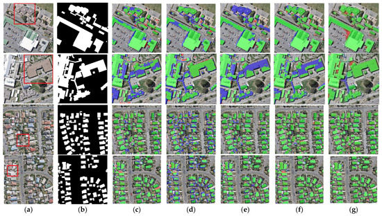
Figure 8.
Examples of building extraction results obtained by different networks on the WHU dataset. (a) Original image. (b) Ground-truth. (c) FCN8s. (d) DANet. (e) SegNet. (f) U-Net. (g) BGC-Net. Note, in Columns (b–g), black, white, green, blue, and red indicate true, false, true-positive, false-negative, and false-positive, respectively. The red rectangles in (a) are the selected regions for close-up inspection in Figure 8.
The first row of Figure 8 represents the extraction results of different networks for multi-scale buildings. For this scene, only BGC-Net extracted all the buildings completely. The rest of the networks fail to extract the complete internal structure of the buildings, and all of them have missing building interiors. This shows that BGC-Net can efficiently acquire multi-scale context information. The second row of Figure 8 shows the extraction results of different networks for complex buildings. FCN8s, DANet, SegNet and U-Net have different degrees of building omission, which means that these networks are not well capable of extracting buildings with complex and irregular structures. In comparison, BGC-Net enables relatively accurate extraction of the entire building. Unfortunately, all networks failed to accurately identify the “Y-structure” in the figure. The third and fourth rows of Figure 8 show the extraction results of different networks for the densely distributed small buildings. As shown in Figure 8d, DANet has the worst extraction results. Most of the contour information of the building is missed, and also, some areas with similar spectral values are misclassified as building areas. FCN8s, SegNet and U-Net can extract relatively complete buildings, but there is a problem of too much noise in the non-building areas, i.e., minor misclassification. BGC-Net has solved the above problems very well. Although the edges of the building body are effectively extracted, the non-building area segmentation does not show significant noise and the perception performance is excellent.
The building segmentation details are shown in Figure 9, with the detail area being the red matrix location in Figure 8. As can be seen from the detail figure, FCN8s, DANet, SegNet and U-Net all present an underfitting phenomenon in building extraction, with some building areas not identified and a large number of missing building interiors in the figure. Due to the addition of multi-scale features and long-range contextual information, BGC-Net can effectively improve the extraction accuracy of buildings. BGC-Net can obtain the whole internal structure with only a small amount of noise at the building’s boundary.
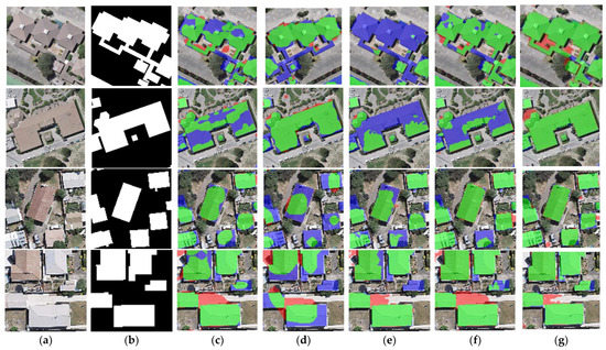
Figure 9.
Close-up views of the results obtained by different networks on the WHU dataset. Images and results shown in (a–g) are the subset from the selected regions marked in Figure 7a. (a) Original image. (b) Ground-truth. (c) FCN8s. (d) DANet. (e) SegNet. (f) U-Net. (g) BGC-Net. Note, in Columns (b–g), black, white, green, blue, and red indicate true, false, true-positive, false-negative, and false-positive, respectively.
4.1.2. Results on CHN Dataset
The results of the building segmentation for different networks on the CHN dataset are shown in Figure 10. From the figure, it is clear that BGC-Net obtains the best segmentation results. Although a few background pixels were misclassified as buildings, the overall extraction effect best matches the ground truth. In contrast, other networks extract buildings with unclear edges. Figure 11 shows the comparison of the building extraction details. As shown in the first row of Figure 11, DANet and SegNet did not extract the buildings in the upper part of the image at all, and FCN8s and U-Net only extracted part of the building. Although BGC-Net detected most of the area of the building, the effect was better than the previous networks. The second row of Figure 11 shows the separate buildings at the edge of the image. The building extraction of FCN8s, DANet and SegNet is incomplete, while U-Net and BGC-Net extract this building accurately. In the third row, BGC-Net can identify buildings partially covered by shadows, while the other networks cannot extract the building areas under shadows at all. In the fourth row, FCN8s and DANet have obvious underfitting and poor extraction. SegNet has a slight underfitting phenomenon, and a few regions are not identified. U-Net and BGC-Net suffer from overfitting, misclassifying gaps as buildings, but BGC-Net has fewer misclassified pixels.
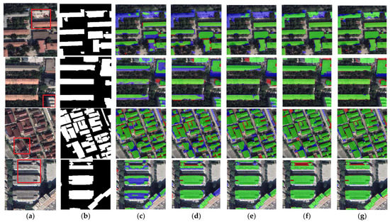
Figure 10.
Examples of building extraction results obtained by different networks on the CHN dataset. (a) Original image. (b) Ground-truth. (c) FCN8s. (d) DANet. (e) SegNet. (f) U-Net. (g) BGC-Net. Note, in Columns (b–g), black, white, green, blue, and red indicate true, false, true-positive, false-negative, and false-positive, respectively. The red rectangles in (a) are the selected regions for close-up inspection in Figure 10.
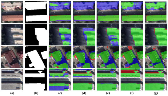
Figure 11.
Close-up views of the results obtained by different networks on the CHN dataset. Images and results shown in (a–g) are the subset from the selected regions marked in Figure 9a. (a) Original image. (b) Ground-truth. (c) FCN8s. (d) DANet. (e) SegNet. (f) U-Net. (g) BGC-Net. Note, in Columns (b–g), black, white, green, blue, and red indicate true, false, true-positive, false-negative, and false-positive, respectively.
The above qualitative analysis shows that, compared with other advanced networks, our proposed BGC-Net is more effective in extracting complex buildings and large buildings in urban environments, and can obtain a more complete internal structure of buildings. It is also possible to accurately extract the edge contours of small buildings. This demonstrates the effectiveness of the proposed network for building extraction in complex urban scenes.
4.2. Quantitative Comparisons
Figure 12 shows a quantitative comparison of the different networks on the urban building dataset. As shown in Figure 12a, our proposed BGC-Net scores higher than other networks on OA, Recall, F1-score and IoU in the WHU dataset. The IoU score of BGC-Net improved by 4.1% (0.89 vs. 0.849) compared to U-Net, which had the next highest overall score performance. In terms of index F1-score scores, BGC-Net improved 2.5%, 12.3%, 10.9% and 7%, respectively, over other models. The above score performance confirms that BGC-Net has a good and stable performance, which could perform the task of extracting buildings from HRAIs satisfactorily. When processing the more challenging CHN dataset, the quantitative evaluation results of each network are shown in Figure 12b. The OA score of BGC-Net is 0.935, Recall score is 0.919, F1-score score is 0.925, and IoU score is 0.861. These four scores are in the first position among all of the network scores. Unfortunately, the Precision score of BGC-Net is only 0.939, which is low compared with other networks, indicating that there is a certain overfitting phenomenon in BGC-Net. It is worth noting that DANet has a lower index than U-Net and SegNet on both datasets. This is because the upsampling process of DANet is simpler. In contrast, SegNet and U-Net use a layer-by-layer feature map recovery strategy in the decoder to obtain better building segmentation results. The above quantitative evaluation shows that BGC-Net is robust, which can effectively handle the task of building extraction in a variety of urban scenes.
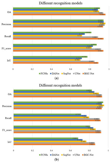
Figure 12.
Quantitative results of different networks on the two datasets. (a) Quantitative results of different networks on the WHU dataset. (b) Quantitative results of different networks on the CHN dataset.
5. Discussion
5.1. Ablation Study
In order to investigate the effects of the AAP module and DGC module on the BGC-Net, ablation experiment is set up in this paper. Based on ResNet-50, three models (ResNet + AAP, ResNet + DGC and ResNet + AAP + DGC) are constructed by different combinations of these two modules. The three models are trained for 150 epochs each under the conditions of computer software, hardware and hyperparameter settings in Section 3.3. The three trained models were tested based on the two datasets.
The extraction results for different module combinations on the WHU dataset are shown in Figure 13. As shown in the first and second rows of Figure 13, the segmentation result of the AAP module has a partial misdetection, misclassifying the surrounding roads as buildings. The DGC module improves this situation, but there is still a small fraction of red pixels in the segmentation result. The combination of the AAP module and DGC module can accurately extract the building, and the false detection is greatly improved. The third row of Figure 13 shows the results of the segmentation of large buildings with different combinations of modules. The AAP module still has a relatively obvious case of false detection, and the DGC module has a partial case of missed detection. Combining the AAP module with the DGC module obtains a clear and accurate outline of the building with no noise.
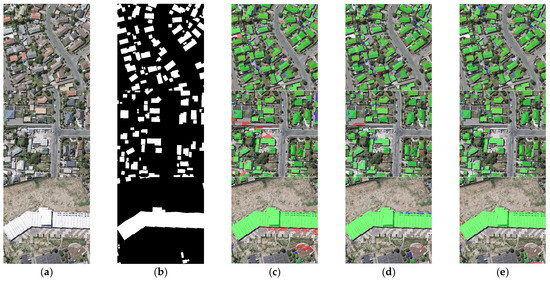
Figure 13.
Comparison of ablation experimental results on the WHU dataset. (a) Original image. (b) Ground-truth. (c) ResNet + AAP. (d) ResNet + DGC. (e) ResNet + AAP + DGC. Note, in Columns (b–e), black, white, green, blue, and red indicate true, false, true-positive, false-negative, and false-positive, respectively.
Table 3 shows the comparison of accuracy evaluation metrics for different modules on the WHU dataset. The comparison shows that the combined AAP and DGC modules have the best accuracy performance, with the IoU score being 7% and 1.3% higher than the AAP and DGC modules alone, respectively. This proves that the combination of the AAP module and the DGC module contributes significantly to the performance of the BGC-Net.
Table 3.
Accuracy statistics of the ablation experiment on the WHU dataset. The best scores are highlighted in bold.
The extraction results for different module combinations on the CHN dataset are shown in Figure 14. As shown in the first row of Figure 14, neither the AAP module nor the DGC module alone identifies the separate building on the right edge of the figure. In contrast, the combination of the AAP module and the DGC module can identify this building. In addition, only the combination of the AAP module and the DGC module identifies the independent building in the lower right corner of the second image. Unfortunately, all three module combinations incorrectly misclassify the shadows between the buildings in the third image as buildings.
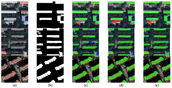
Figure 14.
Comparison of ablation experimental results on the CHN dataset. (a) Original image. (b) Ground truth. (c) ResNet + AAP. (d) ResNet + DGC. (e) ResNet + AAP + DGC. Note, in Columns (b–e), black, white, green, blue, and red indicate true, false, true-positive, false-negative, and false-positive, respectively.
Table 4 shows the comparison of accuracy evaluation metrics for different modules on the CHN dataset. The combination of the AAP module and the DGC module achieved the highest scores on OA, Precision, Recall, F1-score, and IoU. Ablation experiments show that the segmentation performance of the DGC module is better than that of the AAP module. Combining two modules at the same time enables the best building extraction performance.
Table 4.
Accuracy statistics of the ablation experiment on the CHN dataset. The best scores are highlighted in bold.
5.2. Comparing with the State-of-the-Art
In order to verify the advancedness of SCA-Net, we conducted a building extraction comparison experiment with two state-of-the-art networks (ARC-Net [3] and BARNet [27]). ARC-Net includes residual blocks with asymmetric convolution (RBAC) to reduce the computational cost and to shrink the model size. In addition, the multi-scale pyramid pooling modules is used to obtain the multi-scale features. BARNet contains a Denser Atrous Spatial Pyramid Pooling (DASPP) module to capture dense multi-scale building features.
The results of the building segmentation are shown in Figure 15. The first and second rows of Figure 15 show the extraction results of different networks for densely distributed small buildings. Among them, the extraction results of ARC-Net are relatively the worst, with a part of the roads detected as buildings. The extraction results of BARNet and BGC-Net are similar, with only a small number of buildings not extracted. In the third row of the figure, for large buildings, BGC-Net has the best extraction results. Although ARC-Net misclassifies part of the shadows as well as the ground as buildings, BARNet cannot obtain the edge information of buildings well. The quantitative comparison results of different networks are shown in Table 5. BGC-Net has the highest scores in OA, Precision, Recall, F1-score and IoU.
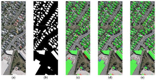
Figure 15.
Building extraction results of different networks on the WHU dataset. (a) Original image. (b) Ground truth. (c) ARC-Net. (d) BARNet. (e) BGC-Net. Note, in Columns (b–e), black, white, green, blue, and red indicate true, false, true-positive, false-negative, and false-positive, respectively.
Table 5.
Average accuracy of different networks for building extraction on WHU dataset. The best scores are highlighted in bold.
5.3. The Effects of Channel Dimension GCN Part
In the DGC module, the channel dimension DGC part interdependencies along the channel dimensions of the network’s feature map, which can obtain more abstract feature information in the image. To test the performance, we conducted a comparison experiment with and without the channel dimension DGC part of BGC-Net on the WHU dataset. As shown in Figure 16, the model without channel dimension GCN does not detect part of the edges of the buildings well. In addition, the model with channel dimension GCN extracts the buildings more completely. As presented in Table 6, the model with channel dimension DGC shows an obvious improvement over the model without channel dimension DGC across all evaluation metrics. The comparison result demonstrates the necessity of the channel dimension GCN part as part of GCN.
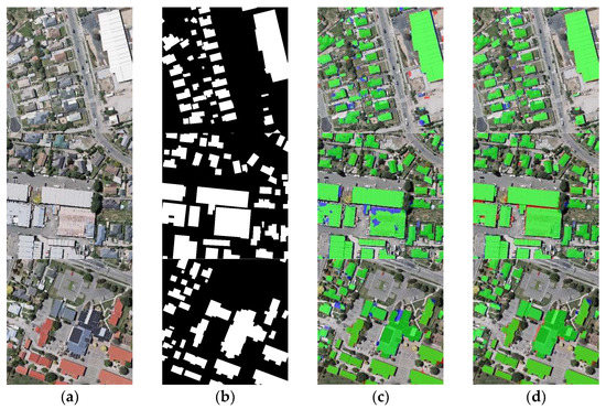
Figure 16.
Comparison of the BGC-Net with or without the channel dimension DGC part on the WHU dataset. (a) Original image. (b) Ground truth. (c) Without channel dimension DGC. (d) Without channel dimension DGC. Note, in Columns (b–d), black, white, green, blue, and red indicate true, false, true-positive, false-negative, and false-positive, respectively.
Table 6.
Average accuracy of the BGC-Net with or without the channel dimension DGC part on the WHU dataset. The best scores are highlighted in bold.
5.4. Limitations
Although the BGC-Net proposed in this paper exhibits good performance, there are still some shortcomings. As shown in Table 7, the number of parameters and computation of BGC-Net is 79.73 M and 29.46 G Mac, respectively, which exceeds the number of parameters of some conventional networks, such as SegNet (16.31 M and 23.77 G Mac) and U-Net (13.4 M and 23.77 G Mac). Second, our network is relatively inefficient. BGC-Net trains an epoch on the WHU dataset and CHN dataset in 256 s and 294 s, respectively, which prevents our network from achieving real-time building segmentation. Therefore, we intend to further simplify the model structure in the future to improve the network efficiency with guaranteed performance. Finally, our network relies on a large amount of labeled data. Therefore, we will explore semi-supervised learning and data augmentation techniques.
Table 7.
Parameters, computation, and training time of each model in WHU dataset and CHN dataset. The best scores are highlighted in bold.
6. Conclusions
In order to better obtain contextual information, this paper combines DFCN and GCN, and proposes the BGC-Net network for the semantic segmentation of buildings. In BGC-Net, the residual module is used to efficiently extract the primary features of the input image. Meanwhile, the attention mechanism is embedded into the pyramid structure to build the AAP module, in order to obtain the multi-scale features of the building more accurately. Moreover, the DGC module is developed based on GCN to model contextual information in space and channels, enhancing the network’s description of the detailed parts of the building. Extensive experiments were conducted on the WHU dataset and the CHN dataset. The results show that BGC-Net can effectively extract a building in a variety of complex urban scenes, outperforming several of the high-performance networks compared. In addition, we explored the impact of each module on the network performance through ablation experiments. The proposed workflow and experimental results highlight the potential of deep learning for rapid and efficient building extraction in complex urban scenes and can provide a theoretical reference for related work.
In this study, compared with other networks, BGC-Net can extract complete large buildings and clear building edges, but there are some limitations. With the introduction of the multiscale module and the graph convolution module, the number of parameters to be trained in the network increases subsequently, making the overall training time of the network longer. In our future work, we will conduct in-depth research in network lightweighting to better balance the efficiency and performance. Simultaneously, we will explore semi-supervised learning techniques to reduce the data cost of deep learning.
Author Contributions
Conceptualization, W.Z. and M.Y.; methodology, W.Z. and X.C.; software, W.Z. and X.C.; validation, W.Z. and M.Y.; formal analysis, M.Y.; investigation, W.Z.; resources, M.Y. and F.Z.; data curation, W.Z. and J.R.; writing—original draft preparation, M.Y.; writing—review and editing, W.Z.; visualization, W.Z.; supervision, M.Y. and H.X.; project administration, M.Y.; funding acquisition, M.Y. and S.X. All authors have read and agreed to the published version of the manuscript.
Funding
This research was financially supported by the China National Key R&D Program during the 13th Five-year Plan Period (Grant No. 2019YFD1100800) and the National Natural Science Foundation of China (41801308).
Data Availability Statement
WHU dataset available at http://gpcv.whu.edu.cn/data/ (accessed on 21 June 2022); CHN dataset available at https://www.scidb.cn/en/detail?dataSetId=806674532768153600&dataSetType=journal (accessed on 21 June 2022).
Acknowledgments
The authors would like to thank the team from Wuhan University and China University of Geosciences (Wuhan) for providing the remote sensing dataset used in this study.
Conflicts of Interest
The authors declare no conflict of interest.
References
- Wu, T.; Hu, Y.; Peng, L.; Chen, R. Improved Anchor-Free Instance Segmentation for Building Extraction from High-Resolution Remote Sensing Images. Remote Sens. 2020, 12, 2910. [Google Scholar] [CrossRef]
- Zhou, J.; Liu, Y.; Nie, G.; Cheng, H.; Yang, X.; Chen, X.; Gross, L. Building Extraction and Floor Area Estimation at the Village Level in Rural China via a Comprehensive Method Integrating UAV Photogrammetry and the Novel EDSANet. Remote Sens. 2022, 14, 5175. [Google Scholar] [CrossRef]
- Liu, Y.; Zhou, J.; Qi, W.; Li, X.; Gross, L.; Shao, Q.; Zhao, Z.; Ni, L.; Fan, X.; Li, Z. ARC-Net: An Efficient Network for Building Extraction from High-Resolution Aerial Images. IEEE Access 2020, 8, 154997–155010. [Google Scholar] [CrossRef]
- Moya, L.; Perez, L.R.M.; Mas, E.; Adriano, B.; Koshimura, S.; Yamazaki, F. Novel Unsupervised Classification of Collapsed Buildings Using Satellite Imagery, Hazard Scenarios and Fragility Functions. Remote Sens. 2018, 10, 296. [Google Scholar] [CrossRef]
- Sun, S.; Mu, L.; Wang, L.; Liu, P.; Liu, X.; Zhang, Y. Semantic Segmentation for Buildings of Large Intra-Class Variation in Remote Sensing Images with O-GAN. Remote Sens. 2021, 13, 475. [Google Scholar] [CrossRef]
- Liu, Y.; Gross, L.; Li, Z.; Li, X.; Fan, X.; Qi, W. Automatic Building Extraction on High-Resolution Remote Sensing Imagery Using Deep networks for biomedical image segmentation Encoder-Decoder with Spatial Pyramid Pooling. IEEE Access 2019, 7, 128774–128786. [Google Scholar] [CrossRef]
- Shackelford, A.K.; Davis, C.H. A Combined Fuzzy Pixel-Based and Object-Based Approach for Classification of High-Resolution Multispectral Data over Urban Areas. IEEE Trans. Geosci. Remote Sens. 2003, 41, 2354–2363. [Google Scholar] [CrossRef]
- Hossain, M.D.; Chen, D. Segmentation for Object-Based Image Analysis (OBIA): A Review of Algorithms and Challenges from Remote Sensing Perspective. ISPRS J. Photogramm. Remote Sens. 2019, 150, 115–134. [Google Scholar] [CrossRef]
- Wang, J.; Yang, X.; Qin, X.; Ye, X.; Qin, Q. An Efficient Approach for Automatic Rectangular Building Extraction from Very High Resolution Optical Satellite Imagery. IEEE Geosci. Remote Sens. Lett. 2014, 12, 487–491. [Google Scholar] [CrossRef]
- Lin, C.; Nevatia, R. Building Detection and Description from a Single Intensity Image. Comput. Vis. Image Underst. 1998, 72, 101–121. [Google Scholar] [CrossRef]
- Huang, D.; Sun, J.; Liu, S.; Xu, S.; Liang, S.; Li, C.; Wang, Z. Multi-dimension and multi-granularity segmentation of remote sensing image based on improved otsu algorithm. In Proceedings of the 2017 IEEE 14th International Conference on Networking, Sensing and Control (ICNSC), Calabria, Italy, 16–18 May 2017; IEEE: New York, NY, USA, 2017; pp. 679–684. [Google Scholar]
- Du, J.; Chen, D.; Wang, R.; Peethambaran, J.; Mathiopoulos, P.T.; Xie, L.; Yun, T. A Novel Framework for 2.5-D Building Contouring from Large-Scale Residential Scenes. IEEE Trans. Geosci. Remote Sens. 2019, 57, 4121–4145. [Google Scholar] [CrossRef]
- Awrangjeb, M.; Zhang, C.; Fraser, C.S. Automatic Extraction of Building Roofs Using LIDAR Data and Multispectral Imagery. ISPRS J. Photogramm. Remote Sens. 2013, 83, 1–18. [Google Scholar] [CrossRef]
- Cui, W.; Zhang, Y. An Effective Graph-Based Hierarchy Image Segmentation. Intell. Autom. Soft Comput. 2011, 17, 969–981. [Google Scholar] [CrossRef]
- Chaokui, L.; Jun, F.; Baiyan, W.; Jianhui, C. Research on the Classification of High Resolution Image Based on Object-Oriented and Class Rule. Int. Arch. Photogramm. Remote Sens. Spat. Inf. Sci. 2015, 7, 75–80. [Google Scholar] [CrossRef]
- Li, C.; Dong, X.; Zhang, Q. Multi-scale object-oriented building extraction method of Tai’an city from high resolution image. In Proceedings of the 2014 Third International Workshop on Earth Observation and Remote Sensing Applications (EORSA), Changsha, China, 11–14 June 2014; IEEE: New York, NY, USA, 2014; pp. 91–95. [Google Scholar]
- Yan, Z.; Huazhong, R.; Desheng, C. The research of building earthquake damage object-oriented change detection based on ensemble classifier with remote sensing image. In Proceedings of the IGARSS 2018—2018 IEEE International Geoscience and Remote Sensing Symposium, Valencia, Spain, 22–27 July 2018; IEEE: New York, NY, USA, 2018; pp. 4950–4953. [Google Scholar]
- Alshehhi, R.; Marpu, P.R.; Woon, W.L.; Dalla Mura, M. Simultaneous Extraction of Roads and Buildings in Remote Sensing Imagery with Convolutional Neural Networks. ISPRS J. Photogramm. Remote Sens. 2017, 130, 139–149. [Google Scholar] [CrossRef]
- LeCun, Y.; Bottou, L.; Bengio, Y.; Haffner, P. Gradient-Based Learning Applied to Document Recognition. Proc. IEEE 1998, 86, 2278–2324. [Google Scholar] [CrossRef]
- Krizhevsky, A.; Sutskever, I.; Hinton, G.E. Imagenet Classification with Deep Convolutional Neural Networks. Adv. Neural Inf. Process. Syst. 2012, 25, 84–90. [Google Scholar] [CrossRef]
- Simonyan, K.; Zisserman, A. Very Deep Convolutional Networks for Large-Scale Image Recognition. arXiv 2014, arXiv:1409.1556. [Google Scholar]
- Long, J.; Shelhamer, E.; Darrell, T. Fully convolutional networks for semantic segmentation. In Proceedings of the IEEE Conference on Computer Vision and Pattern Recognition, Boston, MA, USA, 7–12 June 2015; pp. 3431–3440. [Google Scholar]
- Ronneberger, O.; Fischer, P.; Brox, T. U-Net: Convolutional networks for biomedical image segmentation. In Proceedings of the International Conference on Medical Image Computing and Computer-Assisted Intervention, Munich, Germany, 5–9 October 2015; Springer: Cham, Switzerland, 2015; pp. 234–241. [Google Scholar]
- Badrinarayanan, V.; Kendall, A.; Cipolla, R. Segnet: A Deep Convolutional Encoder-Decoder Architecture for Image Segmentation. IEEE Trans. Pattern Anal. Mach. Intell. 2017, 39, 2481–2495. [Google Scholar] [CrossRef]
- Noh, H.; Hong, S.; Han, B. Learning deconvolution network for semantic segmentation. In Proceedings of the IEEE International Conference on Computer vision, Washington, DC, USA, 7–13 December 2015; pp. 1520–1528. [Google Scholar]
- Yu, M.; Zhang, W.; Chen, X.; Liu, Y.; Niu, J. An End-to-End Atrous Spatial Pyramid Pooling and Skip-Connections Generative Adversarial Segmentation Network for Building Extraction from High-Resolution Aerial Images. Appl. Sci. 2022, 12, 5151. [Google Scholar] [CrossRef]
- Jin, Y.; Xu, W.; Zhang, C.; Luo, X.; Jia, H. Boundary-Aware Refined Network for Automatic Building Extraction in Very High-Resolution Urban Aerial Images. Remote Sens. 2021, 13, 692. [Google Scholar] [CrossRef]
- Pan, X.; Gao, L.; Zhang, B.; Yang, F.; Liao, W. High-Resolution Aerial Imagery Semantic Labeling with Dense Pyramid Network. Sensors 2018, 18, 3774. [Google Scholar] [CrossRef] [PubMed]
- Liu, H.; Luo, J.; Huang, B.; Hu, X.; Sun, Y.; Yang, Y.; Xu, N.; Zhou, N. DE-Net: Deep Encoding Network for Building Extraction from High-Resolution Remote Sensing Imagery. Remote Sens. 2019, 11, 2380. [Google Scholar] [CrossRef]
- Ji, S.; Wei, S.; Lu, M. A Scale Robust Convolutional Neural Network for Automatic Building Extraction from Aerial and Satellite Imagery. Int. J. Remote Sens. 2019, 40, 3308–3322. [Google Scholar] [CrossRef]
- Liu, Y.; Zhu, Q.; Cao, F.; Chen, J.; Lu, G. High-Resolution Remote Sensing Image Segmentation Framework Based on Attention Mechanism and Adaptive Weighting. ISPRS Int. J. Geo-Inf. 2021, 10, 241. [Google Scholar] [CrossRef]
- Zhu, Q.; Liao, C.; Hu, H.; Mei, X.; Li, H. MAP-Net: Multiple Attending Path Neural Network for Building Footprint Extraction from Remote Sensed Imagery. IEEE Trans. Geosci. Remote Sens. 2020, 59, 6169–6181. [Google Scholar] [CrossRef]
- Sun, G.; Huang, H.; Zhang, A.; Li, F.; Zhao, H.; Fu, H. Fusion of Multiscale Convolutional Neural Networks for Building Extraction in Very High-Resolution Images. Remote Sens. 2019, 11, 227. [Google Scholar] [CrossRef]
- Zhang, Z.; Huang, J.; Jiang, T.; Sui, B.; Pan, X. Semantic Segmentation of Very High-Resolution Remote Sensing Image Based on Multiple Band Combinations and Patchwise Scene Analysis. J. Appl. Remote Sens. 2020, 14, 16502. [Google Scholar] [CrossRef]
- Guo, M.; Liu, H.; Xu, Y.; Huang, Y. Building Extraction Based on U-Net with an Attention Block and Multiple Losses. Remote Sens. 2020, 12, 1400. [Google Scholar] [CrossRef]
- Zhang, F.; Chen, Y.; Li, Z.; Hong, Z.; Liu, J.; Ma, F.; Han, J.; Ding, E. Acfnet: Attentional class feature network for semantic segmentation. In Proceedings of the IEEE/CVF International Conference on Computer Vision, Seoul, Republic of Korea, 27 October–2 November 2019; pp. 6798–6807. [Google Scholar]
- He, K.; Zhang, X.; Ren, S.; Sun, J. Deep residual learning for image recognition. In Proceedings of the IEEE Conference on Computer Vision and Pattern Recognition, Las Vegas, NA, USA, 27–30 June 2016; pp. 770–778. [Google Scholar]
- Chen, L.-C.; Papandreou, G.; Kokkinos, I.; Murphy, K.; Yuille, A.L. Deeplab: Semantic Image Segmentation with Deep Convolutional Nets, Atrous Convolution, and Fully Connected Crfs. IEEE Trans. Pattern Anal. Mach. Intell. 2017, 40, 834–848. [Google Scholar] [CrossRef]
- Zhao, H.; Shi, J.; Qi, X.; Wang, X.; Jia, J. Pyramid scene parsing network. In Proceedings of the IEEE Conference on Computer Vision and Pattern Recognition, Honolulu, HI, USA, 21–26 July 2017; pp. 2881–2890. [Google Scholar]
- Chen, L.-C.; Zhu, Y.; Papandreou, G.; Schroff, F.; Adam, H. Encoder-decoder with atrous separable convolution for semantic image segmentation. In Proceedings of the European Conference on Computer Vision (ECCV), Munich, Germany, 8–14 September 2018; pp. 801–818. [Google Scholar]
- Yang, M.; Yu, K.; Zhang, C.; Li, Z.; Yang, K. Denseaspp for semantic segmentation in street scenes. In Proceedings of the IEEE Conference on Computer Vision and Pattern Recognition, Salt Lake City, UT, USA, 18–22 June 2018; pp. 3684–3692. [Google Scholar]
- Yu, M.; Chen, X.; Zhang, W.; Liu, Y. AGs-Unet: Building Extraction Model for High Resolution Remote Sensing Images Based on Attention Gates U Network. Sensors 2022, 22, 2932. [Google Scholar] [CrossRef] [PubMed]
- Fu, J.; Liu, J.; Tian, H.; Li, Y.; Bao, Y.; Fang, Z.; Lu, H. Dual attention network for scene segmentation. In Proceedings of the IEEE/CVF Conference on Computer Vision and Pattern Recognition, Long Beach, CA, USA, 16–17 June 2019; pp. 3146–3154. [Google Scholar]
- Kang, W.; Xiang, Y.; Wang, F.; You, H. EU-Net: An Efficient Fully Convolutional Network for Building Extraction from Optical Remote Sensing Images. Remote Sens. 2019, 11, 2813. [Google Scholar] [CrossRef]
- Yan, J.; Ji, S.; Wei, Y. A Combination of Convolutional and Graph Neural Networks for Regularized Road Surface Extraction. IEEE Trans. Geosci. Remote Sens. 2022, 60, 1–13. [Google Scholar] [CrossRef]
- Zhang, J.; Hua, Z.; Yan, K.; Tian, K.; Yao, J.; Liu, E.; Liu, M.; Han, X. Joint Fully Convolutional and Graph Convolutional Networks for Weakly-Supervised Segmentation of Pathology Images. Med. Image Anal. 2021, 73, 102183. [Google Scholar] [CrossRef] [PubMed]
- Ouyang, S.; Li, Y. Combining Deep Semantic Segmentation Network and Graph Convolutional Neural Network for Semantic Segmentation of Remote Sensing Imagery. Remote Sens. 2020, 13, 119. [Google Scholar] [CrossRef]
- Yuan, Y.; Huang, L.; Guo, J.; Zhang, C.; Chen, X.; Wang, J. Ocnet: Object Context Network for Scene Parsing. arXiv 2018, arXiv:1809.00916. [Google Scholar]
- Zhang, L.; Li, X.; Arnab, A.; Yang, K.; Tong, Y.; Torr, P.H.S. Dual Graph Convolutional Network for Semantic Segmentation. arXiv 2019, arXiv:1909.06121. [Google Scholar]
- Ji, S.; Wei, S.; Lu, M. Fully Convolutional Networks for Multisource Building Extraction from an Open Aerial and Satellite Imagery Data Set. IEEE Trans. Geosci. Remote Sens. 2018, 57, 574–586. [Google Scholar] [CrossRef]
- Fang, F.; Wu, K.; Zheng, D.; Chen, Y.; Zeng, L.; Zhang, J.; Chai, S.; Xu, W.; Yang, Y.; Li, S.; et al. A Dataset of Building Instances of Typical Cities in China. Chin. Sci. Data 2021, 6, 191–199. [Google Scholar]
- Kingma, D.P.; Ba, J. Adam: A Method for Stochastic Optimization. arXiv 2014, arXiv:1412.6980. [Google Scholar]


Publisher’s Note: MDPI stays neutral with regard to jurisdictional claims in published maps and institutional affiliations. |
© 2022 by the authors. Licensee MDPI, Basel, Switzerland. This article is an open access article distributed under the terms and conditions of the Creative Commons Attribution (CC BY) license (https://creativecommons.org/licenses/by/4.0/).