Impact Assessment of Waste Odor Source Locations on Pedestrian-Level Exposure Risk

Abstract

Poor wind environment in residential areas leads to the accumulation of odor from domestic waste, affecting pedestrian health. A reasonable arrangement of waste collection points can reduce pedestrian exposure risks. This study aims to investigate the hydrogen sulfide (H₂S) dispersion and residents’ exposure risk at the pedestrian level for five different locations of waste collection points in a residential building array. Simulation results are consistent with the benchmark wind tunnel experiment, validating that the used turbulence model and numerical methods show good agreement with the predictions of the aforementioned problem. Results indicate that the dimensionless concentration of H₂S and personal intake fraction in a residential area are lower when the collection point is at the corner of the building array periphery. When the collection point is located in the middle of the periphery of the building array or between two adjacent buildings in the center of the array, the local dimensionless concentration of H₂S is 50 at the pedestrian level, and the personal intake fraction is three orders of magnitude higher than that at the corner of the building array periphery. The findings provide a reference for the layout of waste collection points in high-density residential areas and reduction in outdoor exposure risk.

1. Introduction

With the acceleration of the urbanization process, the formation of high-density urban buildings hinders urban ventilation, affecting outdoor air quality and thermal comfort, which reduces residents’ willingness and expectations to participate in outdoor activities, thereby affecting residents’ health [1,2]. These buildings lead to poor ventilation in the city, which makes the air quality worse and causes various health and comfort problems. In high-density cities, low wind speed conditions cause some problems such as temperature rise and pollutant accumulation in the street canyons [3,4]. In order to improve the pedestrian-level wind (PLW) environment in high-density cities, scholars have summarized a variety of factors affecting PLW. For example, the shape, orientation and location of buildings should be considered at the initial stage of design, which is conducive to improving PLW conditions in urban areas [5]. In addition, the cross-section shape of a single building, the angle between the building and the wind direction, the building width and spacing and the building configuration also affect wind environment and wind comfort at the pedestrian level. Compared with a square building model, the wake region length of building with cut, chamfered and rounded corners is reduced [6]. The smaller the angle between the building and the wind direction, the smaller the wind resistance, and the wind speed will be higher [7]. Tsang et al. [8] argue that building size and spacing can affect the PLW environment, where wider buildings hinder natural ventilation around them, while taller buildings improve near-field ventilation. Zhang et al. [9] found that super-tall buildings in a regular urban area increased the wind speed, and the area with acceptable wind comfort could be affected by changing the building configuration. In order to increase building permeability and improve the weak wind conditions in a high-density city, Liu et al. [10] conducted numerical simulation analysis for buildings with or without a lift-up design, and found that the turbulence intensity and the gust field in the wake area of buildings with the lift-up design were greatly changed. Although there is a wind amplification effect in semi-open space under elevated buildings, this effect will be partially weakened due to the influence of surrounding buildings [11].

The diffusion of pollutants is related to the flow field, and effective urban ventilation can adequately dilute the pollutant concentration between buildings [12]. Studies have shown that the lift-up design could provide local wind corridors and form high wind speed zones to reduce local pollutant concentrations [13]. Normally, the higher the wind speed, the faster the dispersion of pollutants in the street canyon. However, the effect of the wind speed on the dispersion of pollutants differed for different street canyon types [14]. From the study of Jiang et al. [15], it can be found that reducing the aspect ratio of the building is beneficial to reducing the accumulation range of pollutants on the leeward side. A reasonable layout of buildings by changing the building density and the height of adjacent buildings can also reduce the polluted area within the building array [16,17]. In addition, the diffusion of pollutants is related to other factors. Keshavarzian et al. [18,19] studied the concentration distribution of pollutants around high-rise building by changing the cross-section shape of buildings and location of pollution sources. Results showed that the distance and angle of the source and the interaction with the cross-section shape of buildings have an impact on the pollutant diffusion around high-rise buildings. However, even if pollutants were released at the same location, concentration fields will also be different due to the different side ratios of isolated high-rise buildings. The backflow zone behind the building will increase as the side ratio decreases, while the vortex shedding will strengthen, resulting in lower pollutant concentrations [15]. In addition, Reiminger et al. [20] also emphasized that the pollutant diffusion between street canyons is greatly influenced by the ratio of building height and the ratio of street canyon width to windward building height. Compared with modifying the aspect ratio of street canyons, reasonable roof design can effectively remove pollutants around the building [21]. In addition to the location of the pollution source, the shape and layout of the building, the wind direction, wind speed and thermal buoyancy are important factors affecting the pollutant concentration distribution [22,23,24,25,26,27].

Computational fluid dynamics (CFD) is one of the methods frequently used to predict pedestrian wind environment and pollutant diffusion. Tominaga and Hosseinzadeh reported that the simulation results of the RNG k-ε model were more consistent with the wind tunnel data if the mean wind flow pattern is considered, showing that the RNG k-ε model provides better performance for predicting the flow field and concentration distribution around a single building compared with other models of Reynolds-averaged Navier–Stokes (RANS) [28,29]. However, when simulating the wind around the building array, it was found that large eddy simulation (LES) had higher accuracy than RNG k-ε in average velocity and concentration [30]. One typical example is the authors’ previous study [10], investigating that the influence of surrounding buildings on the wind amplification around an elevated building by adopting LES. However, the LES method is very sensitive to the setting of influencing parameters and numerical schemes, and requires long computing time [31]. RANS provides acceptable data of flow and concentration field, and considering the computing time and hardware resources, RANS is still used in nearly 96% of simulation studies on wind environment [32]. It can be seen that RANS is still an economical turbulence modeling approach for the study of pollutant diffusion in residential areas.

In most studies on the diffusion of pollutants around buildings, the harmful components of automobile exhaust (CO, NO_X) are often used as the pollution sources. Note that there are few reports about the odor from domestic wet waste diffusing with the wind in residential areas. Domestic waste is a non-negligible source that exists inside the settlement and emits pollutants at all times. Recently, urban residential areas in several Chinese cities, such as Shanghai and Beijing, have successively implemented waste classification. Due to the large population in the community, a large amount of waste is generated every day. More specifically, in summer, the odors from waste seriously affect the lives of city residents. Among them, wet garbage contains a lot of water, which is easily colonized by microorganisms, producing staphylococcus aureus, tuberculosis bacteria and other pathogenic bacteria, and humans are bitten by insects and flies that swallow the garbage, causing diseases [33]. However, the waste is generated and stored in homes or communities until it is delivered to landfills or elsewhere for disposal (as shown in Figure 1). Volatile organic compounds (VOCs) are produced when the organic components in the waste are biodegraded. VOCs emissions lead to a series of environmental problems such as global warming and ozone depletion, as well as health problems such as respiratory irritation and central nervous system damage, and even increase the risk of cancer [34,35]. In addition, some trace compounds such as sulfur compounds, oxygen compounds and hydrocarbons are also produced [36,37], while garbage odor is mainly related to sulfides [38,39], especially hydrogen sulfide (H₂S). Note that H₂S content is low and unstable, and the concentration gradually decreases over time [40]. However, due to its low threshold, it can have a direct impact on people’s sense of smell and harm residents’ respiratory health at low concentrations. One recent study has shown that effective ventilation can reduce surrounding H₂S concentrations [39]. Therefore, reasonably arranging the locations of waste collection points in a residential area can quickly dilute the odor by natural wind, which is conducive to reducing the exposure risk of garbage odor in the residential area.

This study aims to assess pedestrian exposure risk to garbage odor in a high-density residential area. To this practical end, CFD is used to simulate the wind flow field and the pollutant concentration field around a residential building array and the results are validated against a wind tunnel test. Then, H₂S is used as the tracer gas to analyze different garbage collection point locations’ impact on the pedestrian exposure risk to the garbage odor in the residential area. The manuscript is organized as follows: (1) An introduction to the research background and the research objective is given; (2) the methods used in the present study are introduced with details; (3) results and major findings of the study are presented and discussed; (4) concluding remarks are drawn, and some of the future works are introduced.

2. Methodology

2.1. Turbulence Modeling Approach

The fluid in this study was assumed to be isothermal, steady state and incompressible, and the RNG k-ε model was used to solve Equations (1) and (2):

$$\frac{\partial u_i}{\partial x_i}=0$$

(1)

$$u_j\frac{\partial u_i}{\partial x_j}=-\frac{1}{\rho }\frac{\partial p}{\partial x_i}+\nu \frac{\partial }{\partial x_j}\left(\frac{\partial u_i}{\partial x_j}+\frac{\partial u_j}{\partial x_i}\right)+\frac{\partial }{\partial x_j}\left(-\overline{u_i^{\prime }{u}_j^{\prime }}\right)$$

(2)

where u_i and u_j were velocity components (m/s) of the fluid in the i and the j directions, respectively; ν was kinematic viscosity (m/s²); $-\overline{u_i^{\prime }{u}_j^{\prime }}$ was the Reynolds stress (N). Meanwhile, the component transport equation is shown in Equation (3):

$$\frac{\partial }{\partial x_i}\left(u_i{C}_{\alpha }\right)=\frac{\partial }{\partial x_i}\left[\left(D_{\alpha ,m}+\frac{\mu }{S{c}_t}\right)\frac{\partial C_{\alpha }}{\partial x_i}\right]+Q_{\alpha }$$

(3)

where C_α was the concentration of pollutant α; D_α,m was the molecular diffusion coefficient (m²/s) of pollutant α; Q_α was the source term of pollutant α; Sc_t was the turbulent Schmitt number, 0.7.

2.2. Case Descriptions

2.2.1. Validation Description

In this study, the CEDVAL B1-1 wind tunnel test results of Hamburg University were used for simulation validation, which provided open source data of pollutant diffusion around buildings [41], as shown in Figure 2. The size of the building was 0.15 m (L) × 0.1 m (W) × 0.125 m (H). One of the buildings was set as the source building and had four surface sources on its leeward facade. The location and the size of the surface sources are shown in Figure 2c. Figure 2a,b present the mean wind velocity measurement line l₁ (x/H = 0.8, y/H = 0), and pollutant concentration measurement lines l₂ (y/H = 0.4, z/H = 0.06) and l₃ (y/H = 0.48, z/H = 0.06). The Reynolds number was 3.7 × 10⁴ based on the building height (H). The tracer gas (CO₂) was released uniformly from the four surface sources with a constant average speed of 0.024 m/s, and the dimensionless concentration value Kc was defined as:

$$K_c=\frac{C_{measured}}{C_{source}}\times \frac{U_{ref}\times H^2}{Q_{source}}$$

(4)

where C_measured is the measured tracer gas concentration, ppm; C_source represents the tracer gas concentration at the source of pollution, ppm; U_ref is the wind speed at reference height, 5.28 m/s; H is the building height, 0.125 m; Q_source is the total emission rate of the sources, m³/s.

The computational domain size was 30.4 H × 30 H × 6 H (in Figure 3). There were 5 H from the top boundary of the computational domain to the top of the building model, and 12 H from the lateral boundary of the computational domain to the periphery wall surface of the building array, which satisfied the requirement that the blockage ratio should be less than 3% as recommended in reference [42]. The computational domain was meshed using three different resolutions, namely coarse, medium and fine. The dimensionless minimal grid sizes (the ratio of the minimum near-wall grid size to the building height) were 0.016, 0.008 and 0.004, respectively. The expansion ratio between two consecutive cells was 1.18. Figure 4 shows three sets of total mesh numbers, namely 4.16 million (case RNG-1), 7.14 million (case RNG-2) and 11.08 million (case RNG-3). The non-dimensional wall distances y⁺ of the first near-wall cells were 10, 5.1 and 2.7, respectively.

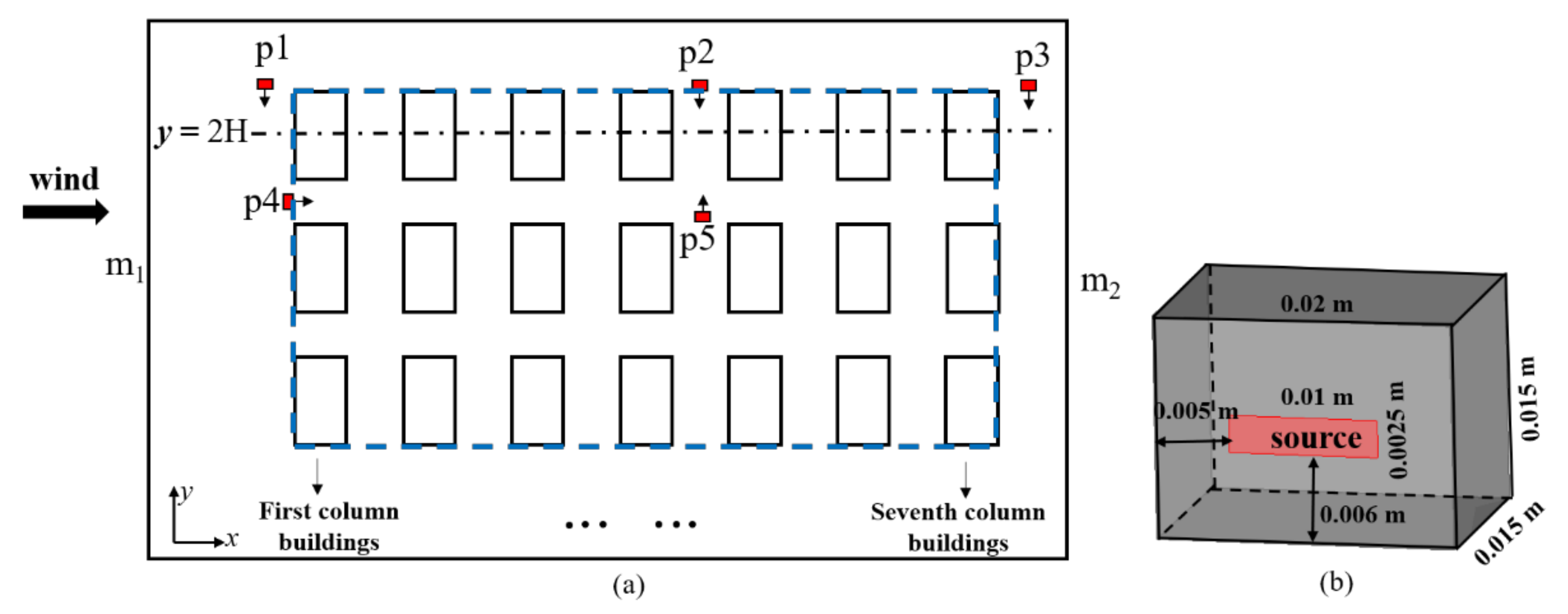
2.2.2. Test Case Description

Taking Shanghai as an example, the locations of waste bins in residential areas should be arranged in a way that they are convenient to the residents [43]. In a typical residential area of Shanghai, the waste collection point is located at the corner of the building array’s periphery, the middle of the array’s periphery and between two adjacent buildings in the center of the building array. The wind tunnel experiment model was used to represent an ideal residential building array configuration. The locations of the waste collection points relative to the building array are shown in Figure 5a: The corner of the building array’s periphery (p1: windward side, p3: leeward side), the middle of the array’s periphery (p2: lateral side, p4: windward side) and between two adjacent buildings in the center of building array (p5). The size of the waste collection point was 4 m (L₁) × 3 m (W₁) × 3 m (H₁), which was simplified to a cube using the same scale of 1:200 as the wind tunnel test model. Pollutants were emitted from a rectangular surface source of 0.01 m × 0.0025 m, located on a facade of the collection point. Arrows in Figure 2a indicate towards which directions the pollutants were emitted, and Figure 2b shows where the surface source was located on the facade. In this study, H₂S was used as the tracer gas. The emission rate of H₂S in a landfill in summer was 4–7 μg/(m²·s) [44], which was affected by waste volume, temperature, ventilation and other factors. Taking the correction coefficient of 50%, the emission rate of H₂S in the residential area was 2–3.5 μg/(m²·s). In this study, 3 μg/(m²·s) was used for subsequent simulation.

2.2.3. Pollutant Exposure Risk Assessment

Pollutant intake fraction (IF) and personal intake fraction (P_IF) are often used to assess the exposure risk of pollutants in residential areas [45,46], and they were defined as shown in Equations (5) and (6):

$$IF={\displaystyle \sum _i^N}{\displaystyle \sum _j^M}{P}_i\times B{r}_{i,j}\times \Delta t_{i,j}\times C{e}_j/m$$

(5)

$$P_{-}IF=IF/{\displaystyle \sum _i^N}{P}_i$$

(6)

where N is defined as the total number of the age groups, and i is the ith age group; M is defined as the total number of microenvironments, and j represents the jth microenvironment; P_i is the total number of people exposed in the ith age group; Br_i,j represents the average volumetric breathing rate for individuals in the jth microenvironment for the ith age group, m³/s; and Δt_i,j is the time spent in the jth microenvironment for the ith age group, s; Ce_j is the concentration of pollutants in the microenvironment j, kg/m³; m is the total emission over the period considered, kg. In this paper, the entire population was divided into three age groups (N = 3): children (21.2%), adults (63.3%) and elderly (15.5%) [45]. Microenvironments were divided into the following four environments (M = 4): indoors at home (j = 1), other indoor locations (j = 2), near-vehicle locations (j = 3) and other outdoor locations (j = 4) [46]. Considering the outdoor exposure risk of residents in the residential area, the outdoor location j = 4 was taken. The volumetric breathing rates Br of children, adults and the elderly were 18.7 m³/day, 20.5 m³/day and 19.5 m³/day, and the times spent on the outdoor locations Δt were 3.9%, 4.7% and 8.6% [45], respectively. The average P_IF (<P_IF >) value at the pedestrian level in the residential area (the blue dotted area in Figure 5a) represented the proportion of the average intake amount per person to the total pollutant emissions.

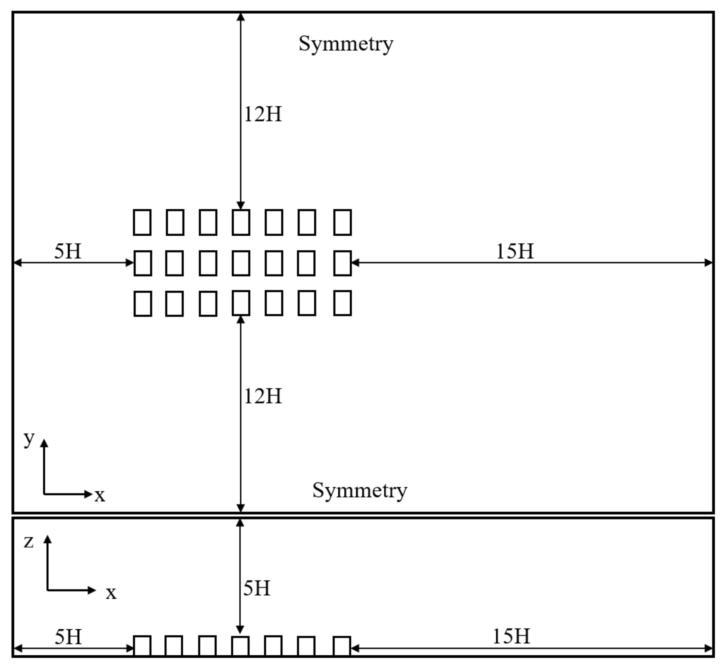
2.3. Boundary Conditions and Numerical Methods

The logarithmic form wind profile was adopted for the inlet condition of the domain [41]. The outlet boundary was set as the pressure outlet, symmetry boundary condition was adopted at the top and the lateral boundaries of the domain and a non-slip condition was adopted at the building surfaces. The details of the inlet wind velocity U, turbulence kinetic energy k and turbulence dissipation rate ε are shown in

Table 1. Boundary conditions in this study.

Names of Boundary Conditions	Settings
Inlet wind velocity (m/s)	$U_{\left(z\right)}=\frac{u^{*}}{\kappa }\times ln\left(\frac{z+z_0}{z_0}\right)$
Turbulence kinetic energy (m2/s2)	$k_{\left(z\right)}=\sqrt{c_1\ln \left(z+z_0\right)+c_2}$
Turbulence dissipation rate (m2/s3)	$\epsilon =C_{\mu }{}^{0.5}{k}_{\left(z\right)}\times \frac{d{u}_{\left(z\right)}}{dz}$
Domain outlet	Pressure outlet
The top and the lateral boundaries of the domain	Symmetry boundary
Building surfaces	Non-slip for wall shear stress

, where the friction velocity u* = 0.3711 m/s, roughness height z₀ = 0.00075 m, empirical constant c₁ = 0.097 and c₂ = 0.516 were obtained by fitting to the wind tunnel results [41]. In addition, the von Kármán constant κ = 0.4187 and model constant C_μ = 0.09 were used. Note that interference from other contaminants was not considered in this study.

ANSYS Fluent 19.0 commercial software was used for calculation in this study. The convection and the diffusion terms were discretized using the second-order upwind scheme. The discretized equations were solved by the SIMPLEC algorithm. The residual of continuity was lower than 10⁻⁴, and the residuals of velocity, k and ε were all lower than 10⁻⁶. After reaching the above residual level criteria, continued calculations showed that the velocity and the pollutant concentration at the monitoring points remained stable.

3. Results and Discussion

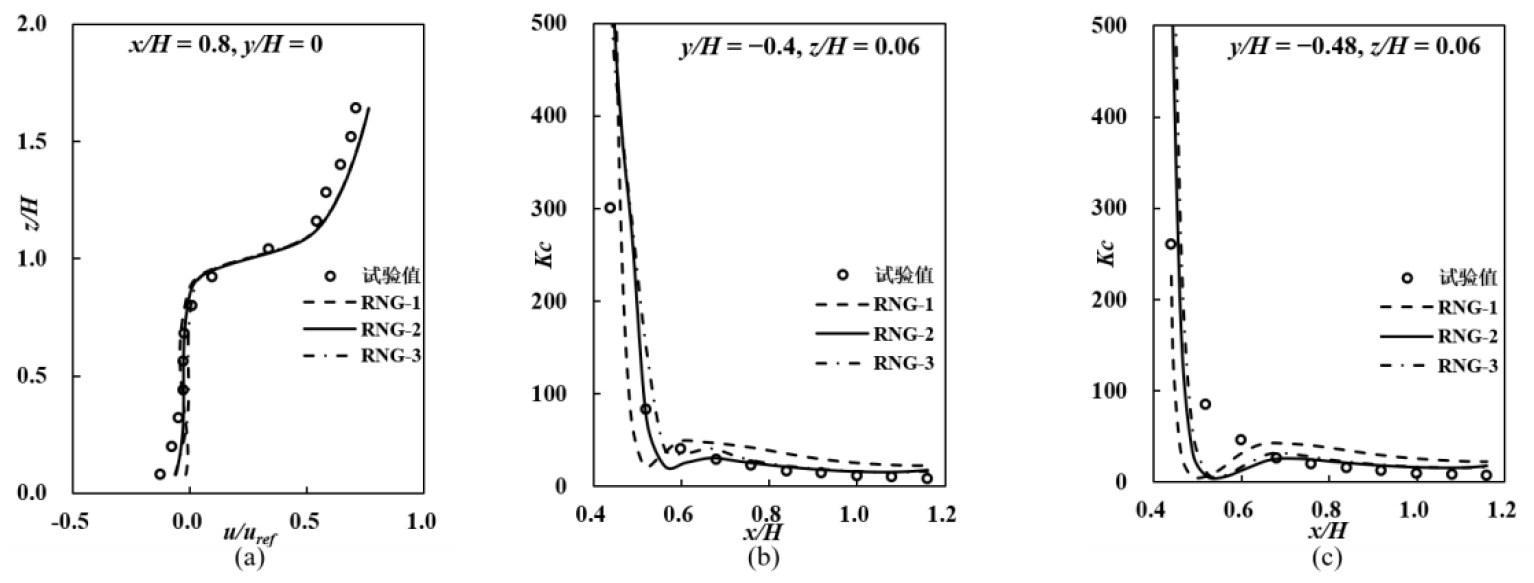
3.1. CFD Validation

Figure 6a shows the mean velocity distribution on the measurement line l₁ along the x direction. The simulation results of the three cases with different mesh numbers are similar and all have a high degree of agreement with the experimental data (EXP) [41]. Figure 6b,c compare the simulated data of pollutant concentration distribution on the measurement lines l₂ and l₃ with the experimental data at the three different grid resolutions. Figure 6b shows that the simulation results of the case RNG-2 and the case RNG-3 are closer to the experimental data. It is worth noting that in the wake region of the building in Figure 6c, x/H = 0.5~0.6, the simulated results are lower than the experimental results [41]. Due to defects in the RNG k-ε model, the pollutant concentrations in the wake zone are underestimated. In general, the simulated results at most locations are more consistent with the experimental data. Therefore, it can be considered that the turbulence model and the numerical method are suitable for the prediction of the diffusion of odor in residential areas. Considering the calculation time and simulation accuracy, the mesh numbers of the following cases are drawn using the meshes of the case RNG-2.

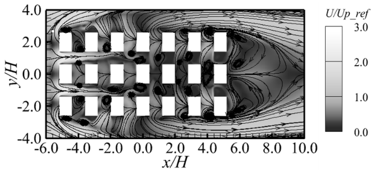
3.2. Pedestrian-Level Mean Flow Field

Figure 7 shows the mean flow field around the residential building array in the X–Y plane. The dimensionless wind speed is the ratio of mean wind speed at pedestrian-level height in the residential area to the wind speed at the same height of the inflow wind. The mean flow field can be divided into low wind speed zone (dark gray, 0.0–1.0), medium wind speed zone (medium gray, 1.0–2.0) and high wind speed zone (light gray, 2.0–3.0). As can be seen from Figure 7, the flow separates upwind to the first column of buildings due to the obstruction of the buildings, and a high wind speed zone appears at this position. The presence of buildings in the residential area led to a gradual decrease in the wind speeds. The medium wind speed zone appears on the leeward side of the first four columns of buildings and the periphery of the building array, while the low wind speed zone appears around the last three columns of buildings. At the same time, there is an obvious wake region at the leeward side of the building array, and when x/H exceeds 8, the effect of the recirculating area is weakened.

3.3. Influence of Source Locations on Concentration Distribution and Exposure Risk

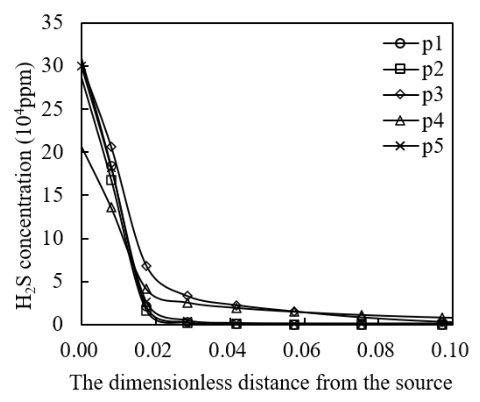
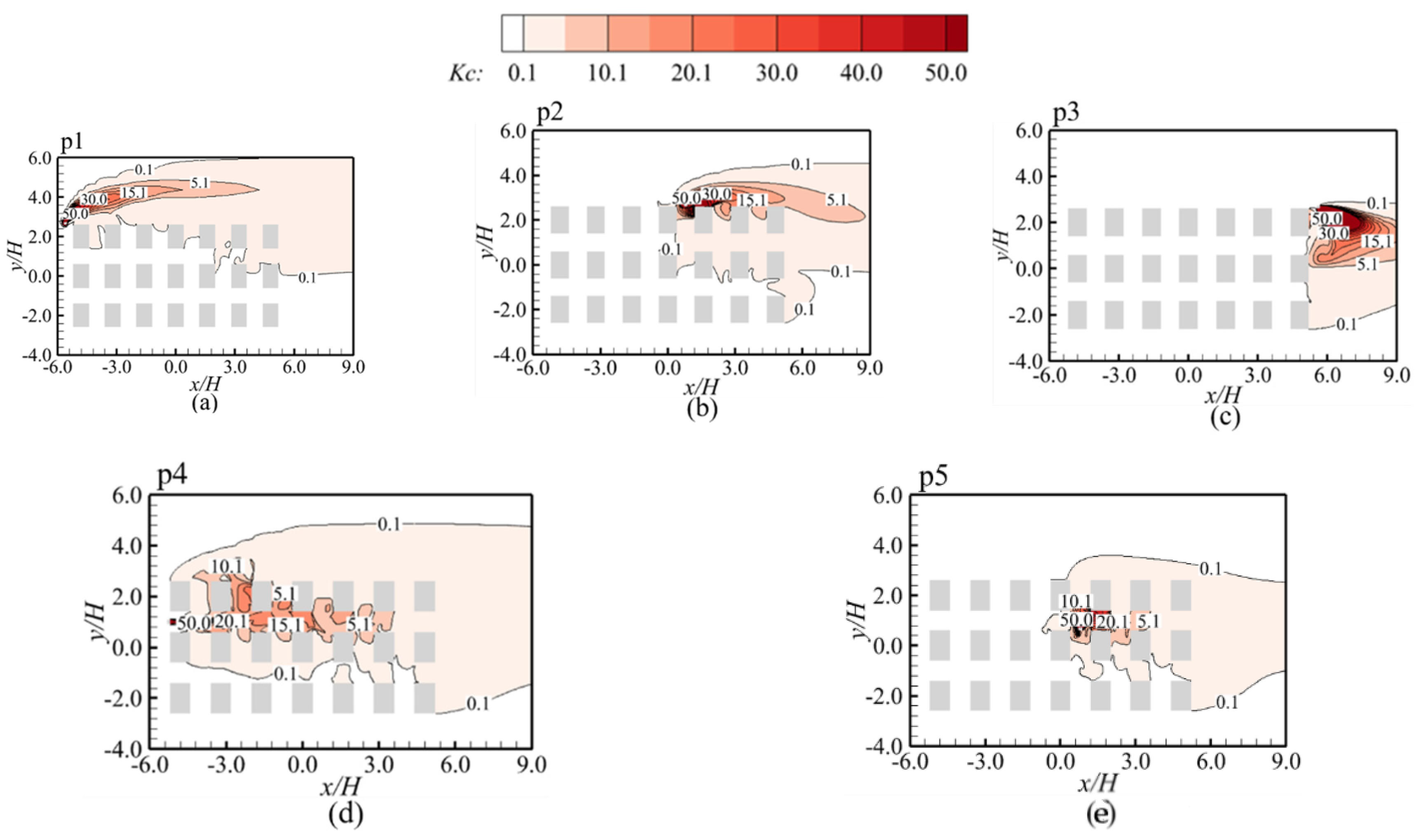
3.3.1. Concentration Distribution of H₂S at Pedestrian Level

Figure 8 shows the H₂S dispersion profiles normal to the surface sources at pedestrian-level height. The distance from the garbage source is made dimensionless by the building height. A sharp decrease in the H₂S concentration within the dimensionless distance of 0.02 is observed for each profile, indicating that the natural wind can quickly dilute the pollutant released at each source location. Especially for the profiles of p1, p2 and p5, the concentrations drop to nearly zero ppm around the dimensionless distance of 0.02.

Figure 9 shows the distributions of H₂S concentration at z/H = 0.06 when the waste collection point is at different locations. As can be seen from Figure 9, when the source is located at p1, the average dimensionless concentration Kc is less than 5 in the residential area, and the area is not fully covered by high-concentration H₂S. This is because p1 is located in the windward side of the corner of the building array’s periphery, where the wind speed is higher and almost unobstructed by the buildings, and the pollutants can be quickly blown to the periphery of the building array by the natural wind. The source at p3 is in the wake region of the building array (Figure 7), and the pollutants tend to accumulate on the leeward side of the adjacent building with low wind speed, which makes the upstream buildings almost unaffected by it.

The release direction of pollutants at p2 is opposite to the wind direction of the location, which causes some pollutants to diffuse with the wind to the periphery of the building array. p5 is located between two adjacent buildings in the middle of the building array, where the wind field is complex and which results in the release of pollutants that cannot be quickly carried away by the wind, forming a local high concentration pollution zone with values of Kc above 50. When the source is located at p4, the pollutants have the widest diffusion range in the residential area. Under the influence of high wind speed, the pollutants rapidly diffuse downstream while being continuously carried by small vortices in the street canyons to the local low wind speed zone of each building.

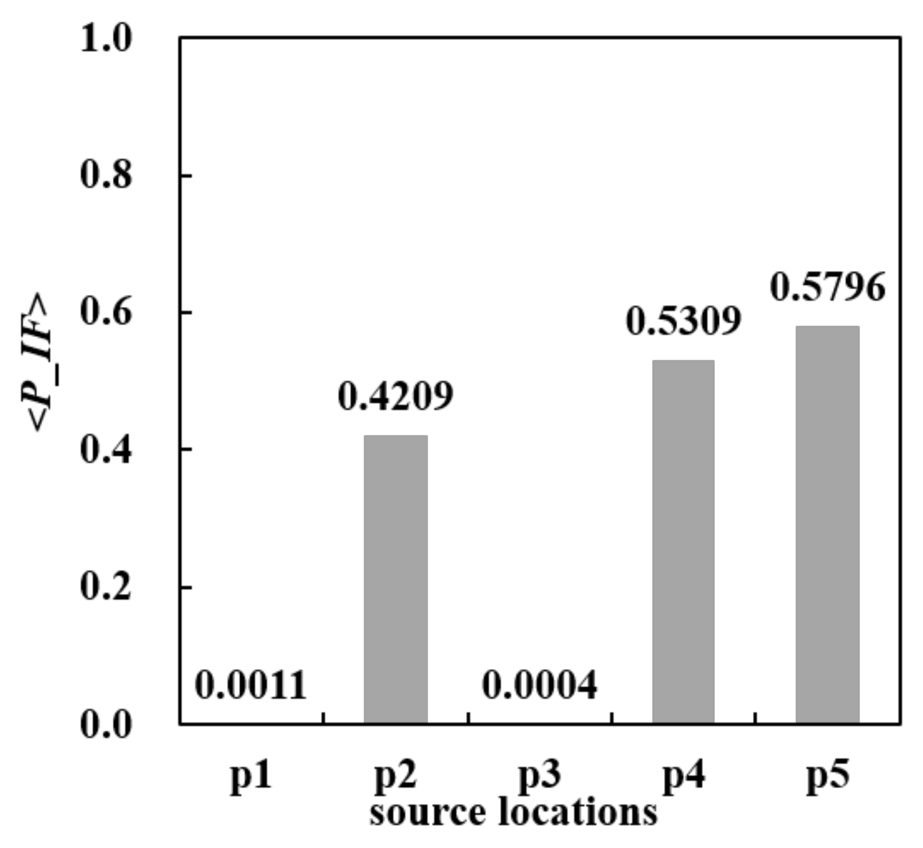
3.3.2. Personal Intake Fraction with Different Source Locations

Figure 10 shows the average personal intake fraction <P_IF> at pedestrian-level height when the source is at different locations. When the source is located at p1 and p3, the <P_IF> is lower, only in the range of 10⁻³–10⁻⁴, which is consistent with the results of lower concentration of H₂S in the residential area in Figure 9a,c. It can be explained as shown in reference [15] that these two locations are located in the separation area and the recirculation area behind the building, and the pollutants mainly exist at the side of the building and near the leeward wall behind the building. Therefore, the pollutant concentration in the residential area is low, while the <P_IF> values of p2, p4 and p5 are in the same order of magnitude and three orders of magnitude higher than the other two locations. The <P_IF> value of p2 is slightly lower than that of p4 and p5, which is caused by the diffusion of some of the pollutants produced by p2 out of the residential area (Figure 9). In the case of p4, the source location is upwind of the building array and the area affected by the pollutant is broader than p5. In the case of p5, the source location is in the center of the building array and its influence is restricted to downwind of the center. However, the <P_IF> value in p4 is lower than p5. The natural wind can quickly disperse the pollutants from p4, but in the case of p5, the pollutant released by p5 is dispersed by the natural wind after it infiltrates into the building array. The natural wind dissipates during the infiltration, causing the pollutant released at p5 to accumulate and resulting in a high <P_IF> value in the residential area. This phenomenon agrees with the reported result [47] that the upwind source location leads to a lower <P_IF>. In addition, the previous study [47] measures the <P_IF> locally within the space between the nearest two buildings, and the present study shows that the upwind source location also results in a lower <P_IF> value for the entire residential area compared to the source location in the center of the residential area. In order to reduce the exposure risk of residents to the odor, it is recommended to avoid arranging the waste collection point in the center of the residential area but to arrange the waste collection point at the area’s periphery, especially at the corners.

4. Conclusions

In this study, the wind driven dispersion of H₂S that released by waste collection points at different locations is investigated in a high-density residential area via CFD simulation. The findings are as follows:

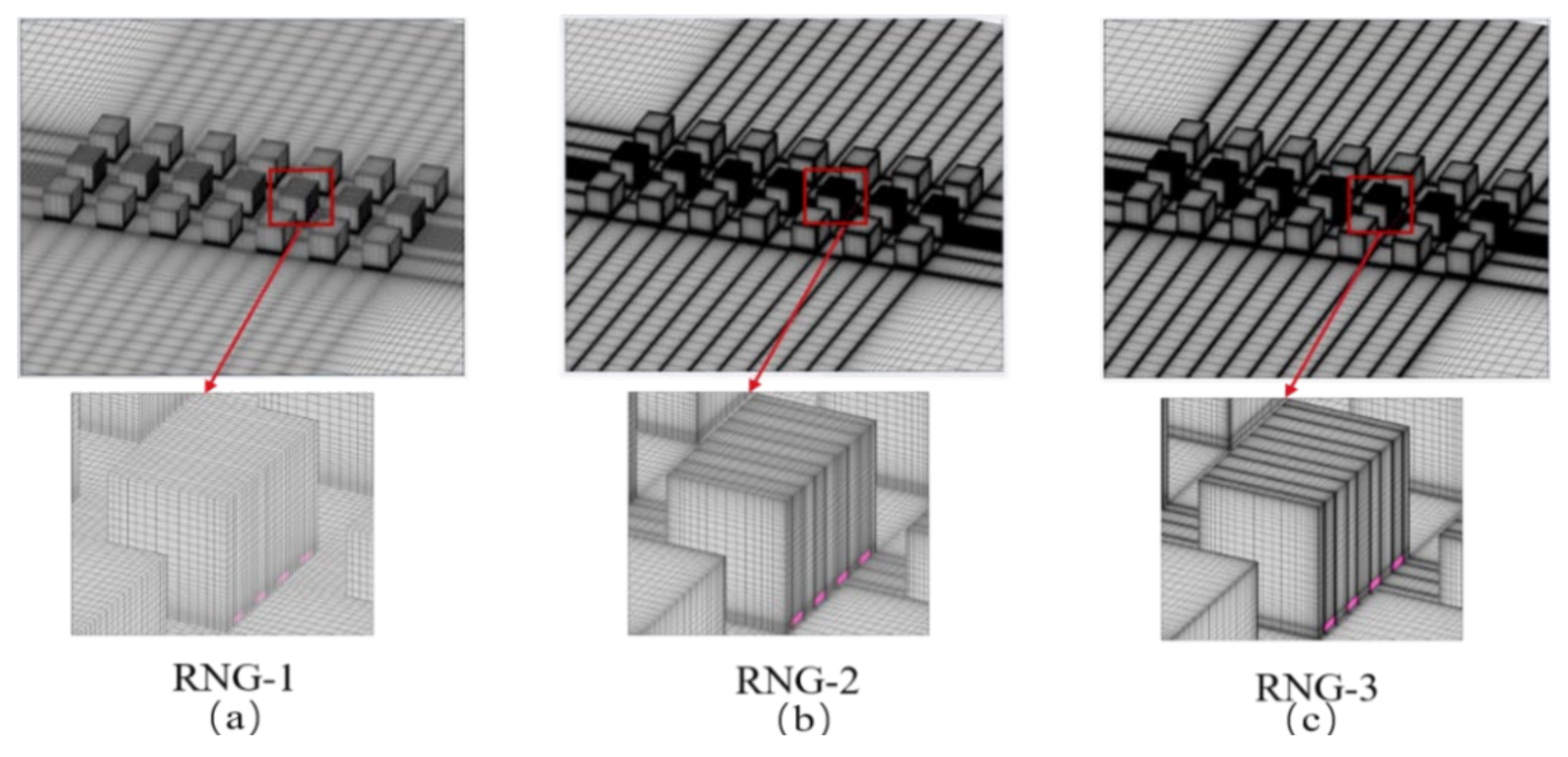
• The simulation results of the wind velocity and pollutant concentration distribution show good agreement with the experimental results, indicating that the RNG k-ε model and used numerical methods are appropriate to predict the diffusion of garbage odor in the residential area.
• High wind speed zones appear on both sides of windward side of the building array. Meanwhile, the buildings show a wind breaking effect, and there are obvious recirculating zones on the leeward side of the building array.
• The exposure risk of residents in the residential area is easily affected by the location of the waste collection point. When the waste collection point is located in the middle of the array’s periphery or between the two adjacent buildings in the center of the building array, outdoor residents are at greater risk of exposure to odors, and the average dimensionless concentration value of H₂S and the personal intake fraction in the pedestrian-level area are one and three orders of magnitude higher than when the waste collection point is located in the corner of the array’s periphery.
• It is recommended to arrange the waste collection point in the corner of the building array’s periphery, not in the middle of the building array’s periphery or between the two adjacent buildings in the center of the array to reduce the exposure risks.

There are still some limitations in the present study. For example, this study only considers one wind direction, and ignores the impact of complex building layout and architectural design on the diffusion of pollutants in residential areas. Meanwhile, other pollutants are also worth exploring on the exposure risk in residential areas in future.

References

1. Zhang, J.; Zhang, F.; Gou, Z.; Liu, J. Assessment of macroclimate and microclimate effects on outdoor thermal comfort via artificial neural network models. Urban Clim. 2022, 42, 101134. [Google Scholar] [CrossRef]
2. Liu, J.; Jiao, J.; Xie, Y.; Xu, Y.; Lin, B. Assessment on the expectation for outdoor usage and its influencing factors. Urban Clim. 2022, 42, 101132. [Google Scholar] [CrossRef]
3. Ai, Z.T.; Mak, C.M. From street canyon microclimate to indoor environmental quality in naturally ventilated urban buildings: Issues and possibilities for improvement. Build. Environ. 2015, 94, 489–503. [Google Scholar] [CrossRef]
4. He, L.; Hang, J.; Wang, X.; Lin, B.; Li, X.; Lan, G. Numerical investigations of flow and passive pollutant exposure in high-rise deep street canyons with various street aspect ratios and viaduct settings. Sci. Total Environ. 2017, 584-585, 189–206. [Google Scholar] [CrossRef] [PubMed]
5. Adamek, K.; Vasan, N.; Elshaer, A.; English, E.; Bitsuamlak, G. Pedestrian level wind assessment through city development: A study of the financial district in Toronto. Sustain. Cities Soc. 2017, 35, 178–190. [Google Scholar] [CrossRef]
6. Mittal, H.; Sharma, A.; Gairola, A. Numerical simulation of pedestrian level wind flow around buildings: Effect of corner modification and orientation. J. Build. Eng. 2019, 22, 314–326. [Google Scholar] [CrossRef]
7. Hong, B.; Lin, B. Numerical studies of the outdoor wind environment and thermal comfort at pedestrian level in housing blocks with different building layout patterns and trees arrangement. Renew. Energy 2015, 73, 18–27. [Google Scholar] [CrossRef]
8. Tsang, C.W.; Kwok, K.C.S.; Hitchcock, P.A. Wind tunnel study of pedestrian level wind environment around tall buildings: Effects of building dimensions, separation and podium. Build. Environ. 2012, 49, 167–181. [Google Scholar] [CrossRef]
9. Zhang, X.; Weerasuriya, A.U.; Zhang, X.; Tse, K.T.; Lu, B.; Li, C.Y.; Liu, C.H. Pedestrian wind comfort near a super-tall building with various configurations in an urban-like setting. Build. Simul. 2020, 13, 1385–1408. [Google Scholar] [CrossRef]
10. Liu, J.; Niu, J.; Mak, C.M.; Xia, Q. Detached eddy simulation of pedestrian-level wind and gust around an elevated building. Build. Environ. 2017, 125, 168–179. [Google Scholar] [CrossRef]
11. Liu, J.; Zhang, X.; Niu, J.; Tse, K.T. Pedestrian-level wind and gust around buildings with a ‘lift-up’ design: Assessment of influence from surrounding buildings by adopting LES. Build. Simul. 2019, 12, 1107–1118. [Google Scholar] [CrossRef]
12. Ma, T.; Xie, X.; Hang, J.; Chen, X.; Xia, X.; Xia, Y. Numerical Study of Inter-unit Dispersion of Pollutant in Single-sided Naturally Ventilated Buildings among Ideal Street Canyon. Build. Sci. 2020, 36, 105–113. [Google Scholar]
13. Sha, C.; Wang, X.; Lin, Y.; Fan, Y.; Chen, X.; Hang, J. The impact of urban open space and ‘lift-up’ building design on building intake fraction and daily pollutant exposure in idealized urban models. Sci. Total Environ. 2018, 633, 1314–1328. [Google Scholar] [CrossRef]
14. Ming, T.; Han, H.; Zhao, Z.; de Richter, R.; Wu, Y.; Li, W.; Wong, N.H. Field synergy analysis of pollutant dispersion in street canyons and its optimization by adding wind catchers. Build. Simul. 2020, 14, 391–405. [Google Scholar] [CrossRef]
15. Jiang, G.; Yoshie, R. Side ratio effects on flow and pollutant dispersion around an isolated high-rise building in a turbulent boundary layer. Build. Environ. 2020, 180, 107078. [Google Scholar] [CrossRef]
16. Zhang, Y.; Ou, C.; Chen, L.; Wu, L.; Liu, J.; Wang, X.; Lin, H.; Gao, P.; Hang, J. Numerical studies of passive and reactive pollutant dispersion in high-density urban models with various building densities and height variations. Build. Environ. 2020, 177, 106916. [Google Scholar] [CrossRef]
17. Cui, D.; Li, X.; Liu, J.; Yuan, L.; Mak, C.M.; Fan, Y.; Kwok, K. Effects of building layouts and envelope features on wind flow and pollutant exposure in height-asymmetric street canyons. Build. Environ. 2021, 205, 108177. [Google Scholar] [CrossRef]
18. Keshavarzian, E.; Jin, R.; Dong, K.; Kwok, K.C.S. Effect of building cross-section shape on air pollutant dispersion around buildings. Build. Environ. 2021, 197, 107861. [Google Scholar] [CrossRef]
19. Keshavarzian, E.; Jin, R.; Dong, K.; Kwok, K.C.S.; Zhang, Y.; Zhao, M. Effect of pollutant source location on air pollutant dispersion around a high-rise building. Appl. Math. Model. 2020, 81, 582–602. [Google Scholar] [CrossRef]
20. Reiminger, N.; Vazquez, J.; Blond, N.; Dufresne, M.; Wertel, J. CFD evaluation of mean pollutant concentration variations in step-down street canyons. J. Wind Eng. Ind. Aerodyn. 2020, 196, 104032. [Google Scholar] [CrossRef]
21. Rafailidis, S. Influence of building areal density and roof shape on the wind characteristics above a town. Bound.-Layer Meteorol. 1997, 85, 255–271. [Google Scholar] [CrossRef]
22. Ghobadi, P.; Nasrollahi, N. Assessment of pollutant dispersion in deep street canyons under different source positions: Numerical simulation. Urban Clim. 2021, 40, 101027. [Google Scholar] [CrossRef]
23. Zhao, S.; Yang, H.; Li, C.; Obadi, I.; Wang, F.; Lei, W.; Xu, T.; Weng, M. Numerical investigation on fire-induced indoor and outdoor air pollutant dispersion in an idealized urban street canyon. Build. Simul. 2021, 15, 597–614. [Google Scholar] [CrossRef]
24. Rong, S.; Wang, P. Simulation of Wind Direction on Numerical Diffusion Particles in Street Canyons Based on DPM Model. Environ. Sci. Technol. 2016, 39, 38–42. [Google Scholar]
25. Shi, T.; Ming, T.; Wu, Y.; Peng, C.; Fang, Y.; de Richter, R. The effect of exhaust emissions from a group of moving vehicles on pollutant dispersion in the street canyons. Build. Environ. 2020, 181, 107120. [Google Scholar] [CrossRef]
26. Zhou, X.; Ying, A.; Cong, B.; Kikumoto, H.; Ooka, R.; Kang, L.; Hu, H. Large eddy simulation of the effect of unstable thermal stratification on airflow and pollutant dispersion around a rectangular building. J. Wind Eng. Ind. Aerodyn. 2021, 211, 104526. [Google Scholar] [CrossRef]
27. Ma, H.; Zhou, X.; Tominaga, Y.; Gu, M. CFD simulation of flow fields and pollutant dispersion around a cubic building considering the effect of plume buoyancies. Build. Environ. 2022, 208, 108640. [Google Scholar] [CrossRef]
28. Tominaga, Y.; Stathopoulos, T. Numerical simulation of dispersion around an isolated cubic building: Comparison of various types of kε models. Atmos. Environ. 2009, 43, 3200–3210. [Google Scholar] [CrossRef]
29. Hosseinzadeh, A.; Keshmiri, A. Computational Simulation of Wind Microclimate in Complex Urban Models and Mitigation Using Trees. Buildings 2021, 11, 112. [Google Scholar] [CrossRef]
30. Tominaga, Y.; Stathopoulos, T. CFD Modeling of Pollution Dispersion in Building Array: Evaluation of turbulent scalar flux modeling in RANS model using LES results. J. Wind Eng. Ind. Aerodyn. 2012, 104–106, 484–491. [Google Scholar] [CrossRef] [Green Version]
31. Liu, J.; Niu, J.; Du, Y.; Mak, C.M.; Zhang, Y. LES for pedestrian level wind around an idealized building array—Assessment of sensitivity to influencing parameters. Sustain. Cities Soc. 2019, 44, 406–415. [Google Scholar] [CrossRef]
32. Toparlar, Y.; Blocken, B.; Maiheu, B.; van Heijst, G.J.F. A review on the CFD analysis of urban microclimate. Renew. Sustain. Energy Rev. 2017, 80, 1613–1640. [Google Scholar] [CrossRef]
33. Jutta, G.; Nazim, U.S.M. Household waste and health risks affecting waste pickers and the environment in low- and middle-income countries. Int. J. Occup. Environ. Health 2017, 23, 299–310. [Google Scholar]
34. Domingo, J.L.; Rovira, J.; Vilavert, L.; Nadal, M.; Figueras, M.J.; Schuhmacher, M. Health risks for the population living in the vicinity of an Integrated Waste Management Facility: Screening environmental pollutants. Sci. Total Environ. 2015, 518–519, 363–370. [Google Scholar] [CrossRef] [PubMed]
35. Li, G.; Sun, H.; Zhang, Z.; An, T.; Hu, J. Distribution profile, health risk and elimination of model atmospheric SVOCs associated with a typical municipal garbage compressing station in Guangzhou, South China. Atmos. Environ. 2013, 76, 173–180. [Google Scholar] [CrossRef]
36. Dincer, F.; Odabasi, M.; Muezzinoglu, A. Chemical characterization of odorous gases at a landfill site by gas chromatography–mass spectrometry. J. Chromatogr. A 2006, 1122, 222–229. [Google Scholar] [CrossRef]
37. Sadowska-Rociek, A.; Kurdziel, M.; Szczepaniec-Cieciak, E.; Riesenmey, C.; Vaillant, H.; Batton-Hubert, M.; Piejko, K. Analysis of odorous compounds at municipal landfill sites. Waste Manag. Res. 2009, 27, 966–975. [Google Scholar] [CrossRef]
38. Wu, C.; Liu, J.; Zhao, P.; Li, W.; Yan, L.; Piringer, M.; Schauberger, G. Evaluation of the chemical composition and correlation between the calculated and measured odour concentration of odorous gases from a landfill in Beijing, China. Atmos. Environ. 2017, 164, 337–347. [Google Scholar] [CrossRef]
39. Colón, J.; Alvarez, C.; Vinot, M.; Lafuente, F.J.; Ponsá, S.; Sánchez, A.; Gabriel, D. Characterization of odorous compounds and odor load in indoor air of modern complex MBT facilities. Chem. Eng. J. 2017, 313, 1311–1319. [Google Scholar] [CrossRef] [Green Version]
40. Papurello, D. Direct injection mass spectrometry technique for the odorant losses at ppb(v) level from nalophan™ sampling bags. Int. J. Mass Spectrom. 2019, 436, 137–146. [Google Scholar] [CrossRef]
41. Leitl, B.; Schatzmann, M. Cedval at Hamburg University. Available online: https://mi-pub.cen.uni-hamburg.de/index.php?id=432 (accessed on 18 April 2022).
42. Tominaga, Y.; Mochida, A.; Yoshie, R.; Kataoka, H.; Nozu, T.; Yoshikawa, M.; Shirasawa, T. AIJ guidelines for practical applications of CFD to pedestrian wind environment around buildings. J. Wind Eng. Ind. Aerodyn. 2008, 96, 1749–1761. [Google Scholar] [CrossRef]
43. He, H.R.; Tang, Y.C. Research on bin design and locating place of ordinary residential area. Shanxi Archit. 2016, 42, 197–198. [Google Scholar]
44. Qiang, N.; Wang, H.Y.; Zhao, A.H.; Yuan, W.X.; Tai, J.; Chen, M. Odor emission rate of municipal solid waste from landfill working area. Build. Sci. 2014, 35, 513–519. [Google Scholar]
45. Luo, Z.; Li, Y.; Nazaroff, W.W. Intake fraction of nonreactive motor vehicle exhaust in Hong Kong. Atmos. Environ. 2010, 44, 1913–1918. [Google Scholar] [CrossRef]
46. Hang, J.; Xian, Z.; Wang, D.; Mak, C.M.; Wang, B.; Fan, Y. The impacts of viaduct settings and street aspect ratios on personal intake fraction in three-dimensional urban-like geometries. Build. Environ. 2018, 143, 138–162. [Google Scholar] [CrossRef]
47. Lin, Y.; Chen, G.; Chen, T.; Luo, Z.; Yuan, C.; Gao, P.; Hang, J. The influence of advertisement boards, street and source layouts on CO dispersion and building intake fraction in three-dimensional urban-like models. Build. Environ. 2019, 150, 297–321. [Google Scholar] [CrossRef]
Figure 1. Domestic waste collection point in a residential area in Shanghai.
Buildings 12 00528 g001
Figure 2. (a) The top view of building model and measurement lines of concentration distribution: (b) The side view of building model and measurement line of wind field; (c) locations and dimensions of the sources.
Buildings 12 00528 g002
Figure 3. The computational domain settings.
Buildings 12 00528 g003
Figure 4. Mesh arrangements: (a) Coarse mesh (case RNG-1); (b) medium mesh (case RNG-2); (c) fine mesh (case RNG-3).
Buildings 12 00528 g004
Figure 5. (a) Source locations; (b) the size of the waste collection point and the discharge port of the source.
Buildings 12 00528 g005
Figure 6. Mean wind velocity and concentration distribution for the cases with different mesh resolutions: (a) The mean wind velocity distribution on measurement line l1; (b) the concentration distribution on measurement line l2; (c) the concentration distribution on measurement line l3.
Buildings 12 00528 g006
Figure 7. Flow field distribution at z/H = 0.06 in X-Y plane.
Buildings 12 00528 g007
Figure 8. Distribution of H2S concentrations away from the source.
Buildings 12 00528 g008
Figure 9. Concentration distributions of H2S in different locations: (a) source location p1; (b) source location p2; (c) source location p3; (d) source location p4; (e) source location p5 at the z/H = 0.06 plane.
Buildings 12 00528 g009
Figure 10. Average personal intake fraction of pedestrian-level height in residential area.
Buildings 12 00528 g010