AlphaTruss: Monte Carlo Tree Search for Optimal Truss Layout Design

Abstract

Truss layout optimization under complex constraints has been a hot and challenging problem for decades that aims to find the optimal node locations, connection topology between nodes, and cross-sectional areas of connecting bars. Monte Carlo Tree Search (MCTS) is a reinforcement learning search technique that is competent to solve decision-making problems. Inspired by the success of AlphaGo using MCTS, the truss layout problem is formulated as a Markov Decision Process (MDP) model, and a 2-stage MCTS-based algorithm, AlphaTruss, is proposed for generating optimal truss layout considering topology, geometry, and bar size. In this MDP model, three sequential action sets of adding nodes, adding bars, and selecting sectional areas greatly expand the solution space and the reward function gives feedback to actions according to both geometric stability and structural simulation. To find the optimal sequential actions, AlphaTruss solves the MDP model and gives the best decision in each design step by searching and learning through MCTS. Compared with existing results from the literature, AlphaTruss exhibits better performance in finding the truss layout with the minimum weight under stress, displacement, and buckling constraints, which verifies the validity and efficiency of the established algorithm.

1. Introduction

A truss is a two or three-dimensional structure that is composed of linear members connected at nodes to sustain loads [1]. Truss layout design aims to find the optimal structural layout considering node locations, connection topology between nodes, and cross-sectional areas of bars [2]. When considering all three aspects simultaneously, numerous design variables and truss layouts are possible. This makes the design of truss layouts challenging. The design process is often represented as a black-box combinational optimization problem, which meets certain criteria, including the material strength, the displacement allowance, the stability of structural members, and other specifications according to different design codes [3]. These constraints are often related to structural performance and require the calculation and analysis of the structural stiffness matrix, which may lead to optimization problems such as non-convexity and non-differentiability [4]. Under such circumstances, how high-level skills can be employed in the automatic design process of complex layout tasks has become a hot and challenging research topic in structural optimization in recent decades [4,5,6]. Many previous studies adopted heuristic search methods to find an approximate global optimal solution, such as a genetic algorithm [7,8,9,10,11], simulated annealing algorithm [12,13], harmony search algorithm [14], particle swarm optimizer [15,16], and so on. However, most metaheuristic algorithms in truss layout problems do not estimate objective functions and apply multiple static searching policies [17], which results in user intervention for appropriate parameter settings.

Reinforcement Learning [17] (RL) is one major kind of machine learning method that deals with the problems interacting between the agent and the environment. An RL algorithm aims to train an agent learning dynamic policies from exploring the environment to maximize the cumulative reward [17]. The training of an agent can be regarded as a trial-and-error process, and the agent gradually learns how to behave better based on the rewards it receives. Monte Carlo Tree Search (MCTS) [18] is a well-known search method to solve RL problems, especially when the reward is received after the final step, which has shown exceptional performance in board games and video games [19]. Alongside AlphaGo [20] and its successors [21,22] in 2016, MCTS-based agents made history by being the first program to beat a professional Go player. It is a landmark event in artificial intelligence that a machine can surpass the vast majority of people in such complex intellectual activity, in which the size of the solution space in Go is as high as 3³⁶¹. The success of MCTS in board games has encouraged researchers to apply it in other scientific fields. Therefore, MCTS has been successfully implemented in video-games [23,24], protein folding problems [25], materials design and discovery [26,27], mixed-integer planning [28,29], and artificial general intelligence for games [30]. However, there exists still only a small number of engineering applications related to MCTS [31,32]. To the best of the authors’ knowledge, no such research has yet applied MCTS in truss layout design problems.

The truss layout design problem is similar to the decision problem of computer Go [19]. On the one hand, the truss layout (the board) is composed of the nodes and edges of the truss (the locations of the Go pieces), and each decision affects the final result in both problems. On the other hand, the final result evaluation can be obtained only after all decisions are made, such as structural weight and winning or losing the game Go. MCTS is a classical approach to solving a Markov Decision Process (MDP) [33] with the evaluation performed at the end of MDP. Therefore, the truss layout design problem may benefit from MCTS by splitting the design process into an MDP, which can provide an environment to give feedback to the current layout.

The main components of an MDP are state, action, transition function, and reward. For the design process of a truss structure, the state refers to the description of the current truss layout. The action contains three sequential types, that is, adding nodes, adding bars, and selecting cross-sectional areas of the bars. For each state, a set of sequential actions are used to describe an available process to reach this state. After taking an action based on the current state, the transition function indicates the probability distribution of the next state. The reward means the evaluation of the action. Based on such an MDP, the truss layouts can be generated by a sequence of actions, which is a basic and simple strategy to expand the solution space and make it more possible to search for innovative solutions. For the truss design process, it is difficult to calculate the reward of an intermediate state if the truss structure is geometrically unstable. Only the layout of a truss structure is determined through a sequence of actions in the terminal state. A reward is then assigned to the generated truss layout, which implies that the reward is always received until the terminal state is reached.

This paper presents an algorithm named AlphaTruss, a novel two-stage reinforcement learning algorithm for optimal truss layout design, which is trained in the MDP environment to give the optimal decision in the design process. AlphaTruss solves the MDP of the truss layout design, finding the optimal sequence of actions by using MCTS with modified upper confidence bound without complex parameter tuning. During the first stage, the design task is modeled as a sequence generation problem in discrete action space to have an approximate optimal layout. In the second stage, AlphaTruss can refine the layout obtained from Stage 1 to get a better solution, where the action only corresponds to node locations and cross-sectional areas of bars, without changing the topology of the truss.

In the following part, Section 2 provides a theoretical background for the methodology on how AlphaTruss algorithm applies MCTS to solve the MDP in the layout design of a truss structure. Section 3 describes four examples of structural layout design considering the material strength, the displacement allowance, the stability of structural members and showing the high performance in comparison with the existing results from the literature. Two analyses and discussions of the MCTS algorithm are presented in Section 4. Section 5 gives several conclusions.

2. Problem and Methodology

2.1. Problem Statement

The truss layout design can be regarded as a black-box problem of combinational optimization, which aims to find the optimal layout by considering node locations, connection topology between nodes, and cross-sectional areas of the bars. A truss layout can be characterized by a set of nodes and bars, denoted as a tuple $\left(P,E\right) | \left(P, E\right)\in \Omega$, where $P$ represents the set of nodes, $E$ represents the set of bars and Ω is the design domain. Each node $u | u\in P$ is a point in Euclidean space (${ℝ}^n, n=2, 3$), and each bar $e | e\in E$ is defined as a tuple $e=\left(u,v,a,\rho \right)$, where $u,v\in P$, $a\in ℝ$ is the cross-sectional area of the bar and $\rho \in ℝ$ is the material density. The design objective is to minimize the total weight of the truss generated under various constraints. This design problem can be formally expressed in Equation (1):

$$\underset{\left(P,E\right)\in \Omega }{\mathrm{minimize}}obj={\displaystyle \sum }_{\left(u,v,a\right)\in E}\rho a{\left|\right|u-v\left|\right|}_2$$

(1)

subject to:

$$g_1:A_{min}\le A_i\le A_{max},i=1,2,\dots ,\left|E\right|$$

$$g_2:{\sigma }_{min}\le {\sigma }_i\le {\sigma }_{max},i=1,2,\dots ,\left|E\right|$$

$$g_3:\left|{\sigma }_i\right|\le {\sigma }_{buckle\_max},i=1,2,\dots ,\left|E_c\right|$$

$$g_4:0\le \left|u_i\right|\le u_{max},i=1,2,\dots ,\left|P\right|$$

$$g_5:Intersect\left(E_i,E_j\right)=False$$

The constraint $g_1$ represents the constraint in the cross-sectional area, which implies that the cross-sectional area $A_i$ should fall within the area interval $\left[A_{min}, A_{max}\right].$The constraint $g_2$ denotes the strength constraint, where ${\sigma }_i$ represents the Mises stress of the bar, and ${\sigma }_{min}$ and ${\sigma }_{max}$ are the maximum allowed compression and tension stresses of the materials. The constraint $g_3$ represents the Euler buckling constraint, where $E_c$ is the set of all bars in compression. ${\sigma }_{buckle\_max}$ is calculated using Euler’s critical load $F_{c{r}_i}$ given in Equations (2) and (3), where $I_i$ is the moment of inertia of the section and $\mu$ represents the length coefficient. For simplicity, the section of all bars is assumed as solid circles, and the length coefficient $\mu$ is 1.0 assuming a pin connection. The constraint $g_4$ denotes the stiffness constraint, where $u_i$ is the maximum displacement in all directions of the $i$^th node. This constraint implies that the displacements at all nodes should not exceed $u_{max}$ in all directions.

$$F_{c{r}_i}=\frac{{\pi }^{2}E{I}_i}{{\left(\mu L_i\right)}^2},i=1,2,\dots ,\left|E_c\right|$$

(2)

$${\sigma }_{buckle\_max}=\frac{F_{c{r}_i}}{A_i},i=1,2,\dots ,\left|E_c\right|$$

(3)

The last constraint $g_5$ implies that any two bars should not intersect with each other. If two bars share one common point at their end, it should not be considered as an intersection. A major omission in the traditional optimization model based on the ground structure method [34] is that the intersection of coplanar bars is allowed. This means that two coplanar solid bars can pass through each other without generating a new node and with no structural effect. However, such intersection of the bars is unusual. Therefore, it is reasonable to avoid such intersection of the bars and consider it as a constraint during the adding-bar steps.

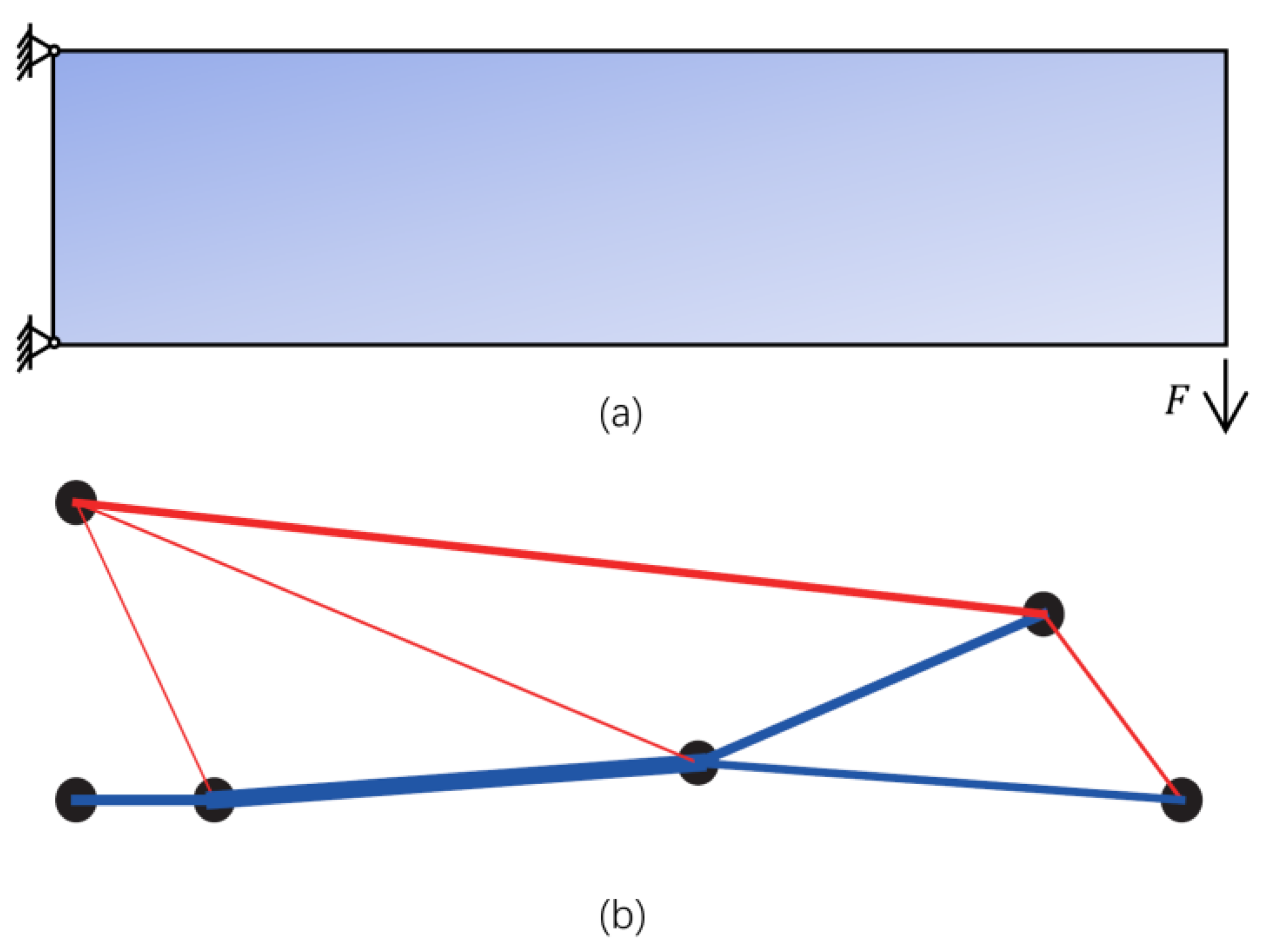
For a specific truss design task, the initial design information and basic design settings are clarified at first. The initial design information includes the positions of the supports, loads, and other fixed nodes defined by users. The basic design settings consist of material data, design domain, and other information required in the design process since the design is constrained by many design metrics. For example, Figure 1 shows a typical truss layout design case for generating a cantilever truss, given the initial design information, such as material properties, load and support conditions (Figure 1a). The task is to find the lightest truss taking stress, displacement, and buckling constraints into account. Figure 1b illustrates a layout solution that will be used in the experiment part (Section 3.1).

2.2. Monte Carlo Tree Search in AlphaTruss

Monte Carlo Tree Search (MCTS) is an iterative, guided, random best-first tree search method that systemically searches a space of candidates to obtain an optimal solution in decision-making problems. Given an MDP $\langle S,A,T,r\rangle$, where $S$ is the set of state $s$, $A$ is the set of action $a$, $T\left(S,a\right):S\times A\to S$ is a transition function, and $r\left(s_{ter}\right)$ is the reward function for a terminal state. MCTS aims to find an optimal action $a$ for a given initial state $s_{init}$ in the MDP model. Figure 2 explains in detail how MCTS is introduced to solve an MDP model with the reward obtained in the final state.

The MCTS method begins with a search tree having only an initial root node built from the given state $s_{init}$. Subsequently, an iterative analysis is performed, expanding the search tree until the search time is terminated. Each iteration consists of four steps [18]: selection, expansion, simulation, and backpropagation.

• Selection: First, starting with $s_{init}$, the algorithm continuously selects actions a according to a strategy of the action selection and transfers them to new states by function $T\left(S,a\right)$ until reaching a new state $S_{new}$, which does not yet exist in the search tree.
• Expansion: The algorithm subsequently expands $S_{new}$ in the search tree base on the selection strategy in selection.
• Simulation: To simulate $s_{new}$, the algorithm follows the Monte Carlo method by randomly taking actions through the function $T\left(S,a\right)$ until arriving at a terminal state $s_{ter}$ and receiving a reward from $r\left(s_{ter}\right)$.
• Backpropagation: Finally, $r\left(s_{ter}\right)$ is used to update information from the new leaf back to the root.

The most common selection strategy for MCTS is the upper confidence bounds [18]. This strategy is applied by using the Chernoff–Hoeffding bounds calculated by Equation (4):

$$I_a=v_a+C\sqrt{\frac{\ln \left({{\displaystyle \sum }}_b{n}_b\right)}{n_a}},$$

(4)

where $v_a$ is the average reward from action $a$ and $n_a$ is the number of actions $a$ that have been applied. ${\displaystyle \sum }_b{n}_b$ implies the total number of simulations so far. The reward term $v_a$ is used to encourage the exploitation of actions with higher reward, while the term $\sqrt{\frac{\ln \left({{\displaystyle \sum }}_b{n}_b\right)}{n_a}}$ is employed to encourage the exploration of actions that are less-visited. $C$ is a heuristic parameter that is empirically set. Usually, $C$ is set as a positive constant, keeping $I_a=+\infty$ when $n_a=0$ initially. This is a standard technique for the application of MCTS [19]. In this study, the value of parameter $C$ is fine-tuned in order to adjust the search width according to different experimental environments.

The MCTS method with the upper confidence bounds is generally called Upper Confidence bounds applied to Trees (UCT). To apply a UCT search to the truss layout design problem, the key step is to formulate the problem to an MDP (Figure 2a). In the MDP of truss layout design, a state $s$ represents the current structural layout and could be denoted by a tuple $\left(P, E\right)$, where $P$ and $E$ are the node and bar set of the structure. A structural layout and a tuple $\left(P, E\right)$ can be mapped to each other. Three different types of actions exist in the action set, i.e., adding a node, adding a bar, and selecting a cross-sectional area (Figure 2b). After taking an action, either set $P$ or set $E$ would change depending on the consequence of the undertaken action. Accordingly, the transition function is defined as the variation of the tuple $\left(P, E\right)$. The reward is the most important part of MCTS, which guides the AlphaTruss algorithm in the right searching direction towards a better solution. In this paper, the reward function is designed to evaluate the action by AlphaTruss, which is based on the theory of structural geometric stability and the results from the structural simulator of Opensees [35]. The details in the reward function are given in the pseudo-code Algorithm 1.

First, whether the structure $\left(P, E\right)$ forms a geometric stable structure or not is to be checked. The function IsStructure is used to conduct this checking task in two steps: evaluation of the Maxwell criterion [36] to calculate the degrees of freedom of $\left(P, E\right)$, and evaluation of the positive definiteness of the stiffness matrix [37] of the structure $\left(P, E\right)$ if the degree of freedom is not larger than 0. If the structure $\left(P, E\right)$is not geometrically stable defined by the function IsStructure, a negative reward of -1 is assigned as a punishment. Otherwise, the function goes through all constraints and checks if the structure $\left(P, E\right)$ satisfies them. If this is not the case, the function receives only a reward of 0. If the structure $\left(P, E\right)$ passes through all the constraints, the function receives a positive reward. Furthermore, the better the objective, the higher reward. Note that the geometric stability is ensured by the IsStructure function. Therefore, it is not included in the constraints part of Equation (1). To check the above-mentioned constraints, the Python package OpenSeesPy [38] is used to conduct all the structural performance calculations, including the constraints $g_2, g_3$ and $g_4$. It is assumed that all truss bars are straight, not curved, and all truss nodes are perfectly hinged.

Algorithm 1 Reward Function for Evaluation
	Input: Node Set $P$, Bar Set $E$  Output: Reward of Structure $\left(P,E\right)$
1:	Function$Reward\left(P, E\right)$//return current action set
2:	If $IsStructure\left(P, E\right)$ then
3:	For every constraint $c$ do
4:	If $\left(P, E\right)$ does not pass $c$ then
5:	Return 0
6:	End For
7:	$obj\leftarrow$ objective of $\left(P,E\right)$
8:	Return $f\left(obj\right)$
9:	Return -1
10:
11:	Function$IsStructure\left(P, E\right)$//check the geometry stability
12:	$d\leftarrow$ dimension of $\left(P, E\right)$
13:	$r\leftarrow$ restricted number of degrees of freedom at support nodes of $\left(P, E\right)$
14:	$N\leftarrow d\times \left|P\right|-\left|E\right|-r$
15:	If $N\le 0$ then
16:	$K\leftarrow$ stiffness matrix of $\left(P, E\right)$
17:	If$K\succ 0$ then
18:	Return True
19:	Return False

In pseudo-code, $f\left(obj\right)$ represents the reward function. For this minimum weight truss design problem, the reward function is defined as $f\left(obj\right)=\lambda /mas{s}^2$, where $\lambda$ is a positive constant to keep the positive rewards matching the negative reward in the same order of magnitude. Based on this MCTS mechanism, the AlphaTruss algorithm adopts a two-stage strategy to find the optimal truss layout, which is introduced in the following two sections.

2.3. Stage I in AlphaTruss for Form-Finding

Stage I in AlphaTruss aims to find an action sequence to form an optimal layout, which will be refined in stage II. In stage I, the design domain of the node locations and cross-sectional areas of the bars are uniformly discretized. The main process of Stage I in AlphaTruss is explained through the pseudo-code Algorithm 2.

Algorithm 2 AlphaTruss Stage I
	Input: Node Set $P$, Bar Set $E$, Allowed Area Interval $I_A$, Number of Nodes $maxp$, Design Domain $D$  Output: Generated Node Set $P_{opt}$, Generated Bar Set $E_{opt}$
1:	$P^{\prime }\leftarrow$ discretized $D$
2:	$E^{\prime }\leftarrow$ all allowed bars
3:	$I^{\prime }\leftarrow$ discretized $I_{\mathrm{A}}$
4:	While$ActionSet\left(P,E\right)\ne \varnothing$do
5:	$a^{*}\leftarrow UCTSearch\left(P, E\right)$
6:	$P, E\leftarrow TakeAction\left(P, E,a^{*}\right)$//modify $\left(P, E\right)$ by taking action $a^{*}$
7:	End While
8:	$P_{opt}, E_{opt}\leftarrow P,E$
9:	Return $P_{opt}, E_{opt}$
10:
11:	Function$ActionSet\left(P, E\right)$//return current action set
12:	If $\left|P\right|<maxp$ then
13:	Return $\left\{add a node p| p\in P^{\prime }-P\right\}$
14:	If $Reward\left(P, E\right)\le 0$ then
15:	Return  $\left\{add a bar e with a=A_{max} | e\in E^{\prime }-E\right\}$
16:	$id\leftarrow$ index of the first unmodified bar
17:	If $id$ exists then
18:	Return  $\left\{Modify area of E_{id} to i | i\in I^{\prime }\right\}$
19:	Return$\varnothing$
20:
21:	Function$UCTSearch\left(P, E\right)$//find an optimal action for $\left(P, E\right)$
22:	While there is time left do
23:	$P_{now}, E_{now}\leftarrow P, E$
24:	While $\left(P_{now}, E_{now}\right)$ is in search tree and $ActionSet\left(P_{now}, E_{now}\right)\ne \varnothing$ do
25:	$A_{now}\leftarrow ActionSet\left(P_{now},E_{now}\right)$
26:	$a_{now}\leftarrow arg{\max }_{a\in A_{now}}{v}_a+C\sqrt{\frac{\ln \left({{\displaystyle \sum }}_{b\in A_{now}}{n}_b\right)}{n_a}}$
27:	$P_{now}, E_{now}\leftarrow TakeAction(P_{now}, E_{now}, a_{now})$
28:	End While
29:	If $\left(P_{now}, E_{now}\right)$ is not in search tree, then
30:	$Expand\left(P_{now}, E_{now}\right)$
31:	$P_{tmp}, E_{tmp}\leftarrow P_{now}, E_{now}$
32:	While $ActionSet\left(P_{tmp}, E_{tmp}\right)\ne \varnothing$ do
33:	$P_{tmp}, E_{tmp}\leftarrow TakeAction\left(P_{tmp}, E_{tmp}, a~ActionSet\left(P_{tmp}, E_{tmp}\right)\right)$
34:	End While
35:	$r=Reward\left(P_{tmp}, E_{tmp}\right)$
36:	While $\left(P_{now}, E_{now}\right) \ne \left(P,E\right)$ do
37:	Use $r$ to update $v_a, n_a$ of $\left(P_{now}, E_{now}\right)$
38:	$P_{now}, E_{now}\leftarrow fa\left( P_{now}, E_{now}\right)$
39:	End While
40:	End While
41:	Return${\mathrm{argmax}}_{a\in ActionSet\left(P,E\right)} v_a$

In stage I, the AlphaTruss algorithm discretizes at first uniformly the design domain (line 1) and the range of the cross-sectional area (line 3) by choosing a certain number of samples from the continuous space.

The available actions vary in different states. The actions are determined by the function ActionSet, which returns an available action set for the current state following the three-step process of truss generation. The first step is to add new structural nodes in the discretized design domain (line 13). The candidate nodes are chosen from the discretized node set. If a sufficient number of nodes have been already added to the node set (line 12), i.e., the number of nodes is equal to $maxp$, the process moves to the second step, that is, adding bars between the nodes (line 15). The adding-bar step ends when a positive reward is received (line 14), i.e., the structure $\left(P,E\right)$ passes all the constraints. To achieve this condition efficiently, the cross-sectional areas of newly added bars are set to the maximum allowed value for more easily fulfilling constraints. The final step is to select the area of each bar according to the adding order of bars (lines 16–18). The area is chosen from the set of the discretized cross-sectional areas. Upon completion, the function ActionSet returns an empty set (line 19), which also indicates that the current state is a terminal one.

After clarifying the action-taking process, the main algorithm (lines 4–7) calls the function UCTSearch to find the optimal action for the current state $\left(P, E\right)$. This state is updated to a new state by applying the optimal action. Then UCTSearch is repeatedly conducted until the terminal state is reached.

The function UCTSearch constitutes the main part of the AlphaTruss in stage I, which follows the four-step repetition described in Figure 2 (Section 2.2). In each iteration, the UCTSearch function selects initially the path to a new leaf node (line 24) using the upper confidence bound formula (line 26). Usually, the evaluation of an action $v_a$ is conducted using the average reward [18]. Since the positive reward is rather sparse and the aim is to find the optimal layout, Equation (5) is used here to estimate $v_a$ by increasing the proportion of the best solution in the evaluation of $v_a$, which combines the average ($\frac{vsu{m}_a}{n_a})$ and best ($vbes{t}_a)$rewards using a parameter $\alpha$. In this study, this parameter is fine-tuned to 0.4. Thus, the final upper confidence bounds used in AlphaTruss can be represented as Equation (6).

$$v_a=\alpha \times \frac{vsu{m}_a}{n_a}+\left(1-\alpha \right)\times vbes{t}_a$$

(5)

$$I_a=\alpha \times \frac{vsu{m}_a}{n_a}+\left(1-\alpha \right)\times vbes{t}_a+C\sqrt{\frac{\ln \left({{\displaystyle \sum }}_b{n}_b\right)}{n_a}}$$

(6)

Subsequently, the algorithm expands the search tree (line 30) and conducts a simulation using the Monte Carlo method (lines 32–34). The pseudo-code $a~ActionSet\left(P_{tmp}, E_{tmp}\right)$ in line 33 represents randomly selected samples from $ActionSet\left(P_{tmp}, E_{tmp}\right)$. At the end of an iteration, the algorithm uses the received reward $r$ (line 35) to update the information from the new leaf to the root (lines 34–37) by maintaining $vsu{m}_a \leftarrow vsu{m}_a+r$, $vbes{t}_a \leftarrow \max \left(vbes{t}_a, r\right)$, $n_a\leftarrow n_a+1$. Finally, the UCTSearch function uses $v_a$ to estimate each candidate action, and it returns the action with the largest $v_a$.

It is known that MCTS is able to give a better MDP decision through more searching time. However, the efficiency of AlphaTruss is also an important issue. Instead of setting the running time for function UCTSearch, the loops are run in AlphaTruss for a certain number of iterations, which is determined by Equation (7):

$$iter\left(i\right)=\{\begin{array}{c}100000, i=0\\ \max \left(50000-1000\times i,20000\right),i>0\end{array}$$

(7)

The variable $i$ is the number of actions taken. Starting from $0$, $i$ is increased by $1$ after every call of the function UCTSearch. For the experiments in this study, the maximum number of iterations in stage I does not exceed ${10}^6$ and these experiments share the same iteration function in stage I as shown in Equation (7).

2.4. Stage II in AlphaTruss for Refinement

When generating a free-form truss layout, the locations of the nodes and the cross-sectional area of the bars are generally continuous. Stage I in AlphaTruss manages these continuous variables by uniformly discretizing these variables. However, this discretization policy restricts the continuous variables from finding a better solution, and the layout obtained in stage I loses its accuracy to a certain degree. To loosen this restriction, Stage II in AlphaTruss is proposed to refine the continuous variables by using a process that is similar to the process in Algorithm 2 (Section 2.3).

Stage II includes two types of action sets: adjusting node locations and adjusting the cross-sectional area of the bar. It requires the layout generated in stage I as an initial layout. Preserving the same topological relations, the node locations and cross-sectional area of the bar are adjusted to improve the layout design. The reward function and constraints are consistent with stage I in AlphaTruss except for the action set.

The first action type is to adjust the position of nodes that are newly added in stage I. The neighborhoods of the nodes are subdivided into several node sets (denoted as neighborhood node sets). Then, new positions of the nodes are chosen from these neighborhood node sets. Similarly, the second action type is to adjust the cross-sectional area of each bar from the input layout, finding the optimal adjustment from each neighborhood area set. Since the connection topology between nodes has already been obtained in stage I, the maximum number of iterations used in stage II is set as half of the one used in stage I for saving the computational budget.

In order to better illustrate this local discretization policy in stage II, Figure 3 shows an example for the generation of the neighborhood node set. The blue dotted lines represent the original truss layout requiring refinement, and the nodes shaded by the blue squares imply that these nodes require position adjustment. The initial truss layout is obtained in stage I of AlphaTruss, where the design domain is uniformly discretized into a 17 × 9 grid distribution. Stage II of AlphaTruss locally adjusts the locations of existing nodes, and the amplitude of each adjustment should not exceed the shaded area of the blue square in Figure 3a, denoted as $\left[-\frac{w}{2},\frac{w}{2}]\times [-\frac{w}{2},\frac{w}{2}\right]$, where $w$ is the step size of the discretization in stage I. Figure 3b shows the newly generated neighborhood node set. A 9 × 9 local subdivision grid pattern is generated in the neighborhood of the considered node. These small neighborhoods make up the candidate node set for each node in the original layout that needs adjustment. For the cross-sectional area, the interval $\left[-\frac{t}{2},\frac{t}{2}\right]$ is divided into 50 pieces to form a candidate set of the cross-sectional area with 51 entries, where $t$ is the step size of the cross-sectional area discretizing in stage I.

Stage II for refinement of AlphaTruss is run for multiple rounds. The refinement process is carried out for at least 10 rounds. After that, the algorithm continues running until either generating a structure with a higher weight than the previous round or reaching 25 rounds. To achieve a better convergence rate, $w\leftarrow 0.9w, t\leftarrow 0.9t$ are used after each round in stage II.

It is worth mentioning that, in this two-stage algorithm, the solution generated by stage I, which is the best one of the ten repeated independent runs in stage I, will be used as the input topology to stage II. The second stage can carry out an effective neighbor-hood search to improve the truss layout based on the topology obtained in stage I.

3. Experiments and Results

Four different experiments involving multiple constraints and load cases are carried out to demonstrate the applicability of the AlphaTruss algorithm in truss layout design problems, which deal with the simultaneous optimization of size, shape, and topology.

3.1. Experiment 1: Proof of Concept

As mentioned, AlphaTruss is implemented by formulating the truss design problem into an action-taking process. Serving as a proof of concept, experiment 1 demonstrates the two-stage design workflow of AlphaTruss. The design domain of the 2D truss layout problem is shown in Figure 4. The details of specified essential nodes (including the nodes for the loadings and supports) are outlined in

Table 1. Essential node information in experiment 1.

Essential Node	Node Location (mm)	Node Label
a	(0, 0)	Pinned Support
b	(0, 2540)	Pinned Support
c	(10,160, 0)	Loaded (0, −444,800 N)

. All five types of constraints ($g_1,g_2,g_3,g_4,g_5$) are used in this experiment.

Table 2. Material properties and constraint parameter settings in experiment 1.

Settings	Experiment 1
Young’s modulus	206,850 MPa (30,000 ksi)
Density	7418.21 kg/m3 (0.268 lb/in3)
Max tension stress	334.6 MPa (50 ksi)
Max compression stress	−334.6 MPa (−50 ksi)
Max node displacement	50.8 mm (2 in)
Min bar area	0.6452 cm2
Max bar area	200 cm2

gives the data of the material properties and constraint settings. The purpose of this experiment is to find the truss layout of minimum weight under stress, displacement, and buckling constraints.

There are three action sets for AlphaTruss to choose sequentially in stage I. In the first action set, nodes are chosen from the candidate node set and added to the structure. The design domain is uniformly discretized into a 17 × 9 grid pattern. In the second action set, several bars are added to the structure until it passes all the constraints. In the third action set, AlphaTruss assigns optimal cross-sectional areas to the generated bars. The cross-sectional area is discretized using a step size of 5 cm² for the allowed range. Figure 5 shows the construction process for the designed truss in stage I of AlphaTruss, which depicts how AlphaTruss makes decisions to build a truss. Note that a bar in red/blue color indicates that it is in tension/compression, respectively. A total of 19 decision steps are required to complete the design, the total number of Monte Carlo simulations is 829,000, which is calculated according to Equation (7).

Stage II of AlphaTruss is used to refine the layout obtained from stage I without changing the connection between the nodes. The details on the refinement settings can be found in Section 2.4. The refinements are conducted by 25 rounds. The weights of the structure after all rounds of refinement are presented in Figure 6. Each round has 11 decision steps since no actions of adding bars are needed, and the number of Monte Carlo simulations per round of stage II is 270,000.

The results show that the rate of decline in the weight gradually decreases after several rounds of refinement. Prior to refinement, the original weight of the structure is 1695.89 kg. After the first 10 rounds of refinement, the original weight is decreased to 1455.62 kg and is reduced by 14.2%. Only minor changes are made by the refinement in each round after the 10th round. However, the weight is still decreased to 1408.47 kg after 25 rounds. The final weight is only 83.0% of the original weight. This implies that the refinement produces a 2.8% decrease in the weight after the 10th round. When considering the computational budget, the experiment results show that a reasonable solution can be achieved after 10 rounds of refinement. If a better solution is desired, more rounds of refinement should be applied. Figure 7 presents the layout after refinement using 25 rounds. The detailed data of the truss are listed in

Table 3. Detailed data of the generated truss in experiment 1.

Node Label	A			B			C
Coordinates (mm)	(8231, 2332)			(6519, 528)			(3037, 0)
Bar Label	1	2	3	4	5	6	7	8
Area (cm2)	51.23	20.65	108.00	100.79	38.24	35.76	59.46	50.41

.

3.2. Experiment 2: Benchmark Test for Size, Shape, and Topology Optimization

In experiment 2, AlphaTruss is tested on the benchmark test of truss layout problem for size, shape, and topology optimization. The design domain is depicted in Figure 8. Two load cases are taken into account. The details of specified essential nodes (including the nodes for the loadings and supports) are listed in

Table 4. Essential node information in experiment 2.

Essential Node	Node Location (mm)	Load Case 1	Load Case 2
a	(0, 0)	Pinned Support	Pinned Support
b	(0, 9144)	Pinned Support	Pinned Support
c	(9144, 0)	Loaded (0, −444,800 N)	Loaded (0, −667,200 N)
d	(18,288, 0)	Loaded (0, −444,800 N)	Loaded (0, −667,200 N)
e	(9144, 9144)	N/A	Loaded (0, 444,800 N)
f	(18,288, 9144)	N/A	Loaded (0, 444,800 N)

for different load cases. Load case 1 has four fixed nodes $\left(a,b,c,d\right)$, whereas load case 2 has six fixed nodes $\left(a,b,c,d,e,f\right)$. The data of the material properties and constraint settings are summarized in

Table 5. Material properties and constraint parameter settings in experiment 2.

Settings	Experiment 2
Young’s modulus	206,850 MPa (30,000 ksi)
Density	7418.21 kg/m3 (0.268 lb/in3)
Max tension stress	334.6 MPa (50 ksi)
Max compression stress	−334.6 MPa (−50 ksi)
Max node displacement	50.8 mm (2 in)
Min bar area	0.6452 cm2
Max bar area *	200 (400) cm2

* When considering the bucking constraint $g_3$, the maximum allowed area is adjusted to 400 cm².

.

The allowed range of the cross-sectional area of the bars is uniformly discretized by a step size of 5 cm². The design domain is discretized into a 17 × 9 grid pattern and 9 × 9 grid pattern in stage I and stage II, respectively (Figure 3). For comparison, the results from Fenton et al. [7] and Petrovic et al. [9] are employed, noting that Fenton et al. [7] considering the buckling constraints, whereas Petrovic et al. [9] did not. Therefore, the same settings are used and two types of constraint combinations (I and II) are selected. Combination I consists of constraints $g_1, g_2, g_4,$ and $g_5$, while combination II adds the buckling constraint $g_3$ to the combination I. The maximum number of nodes in AlphaTruss is set to six in load case I and seven in load case II, which is consistent with the setting in the literature [7,9]. A comparison between the results from AlphaTruss and those from previous studies is given in

Table 6. Experiment 2 results: minimum truss weights (kg).

Algorithm	Fenton, et al. [7]	Petrovic, et al. [9]	AlphaTruss
			Stage I	Stage II
Load case I, Constraint combination I	2217.54	N/A	2210.10	2149.74
Load case I, Constraint combination II	N/A	3252.77	3136.32	2959.89
Load case II, Constraint combination I	2097.54	N/A	1692.10	1616.00
Load case II, Constraint combination II	N/A	N/A	2950.94	2607.07

.

The results indicate that stage I of AlphaTruss generates lighter trusses compared to those generated by the previous studies. It is worth mentioning that stage II reduces further the weights of the trusses by maximum 11.7% for load case II and constraint combination II. The pertinent optimal layouts and data of the generated trusses are illustrated in Figure 9 and

Table 7. Detailed data of the truss layout in experiment 2. (a) Load case I with constraint combination I. (b) Load case I with constraint combination II. (c) Load case II with constraint combination I. (d) Load case II with constraint combination II.

(a)
Node Label	A					B
Coordinates (mm)	(11,324, 7469)					(7066, 3591)
Bar label	1	2	3	4		5	6	7	8
Area (cm2)	88.84	74.66	29.87	115.45		143.86	170.16	106.48	137.31
(b)
Node Label	A					B
Coordinates (mm)	(3535, 0)					(14,037, 4563)
Bar label	1	2	3	4		5	6	7	8
Area (cm2)	136.94	51.67	166.96	121.08		278.26	252.57	226.93	130.28
(c)
Node Label	A
Coordinates (mm)	(18,276, 4584)
Bar label	1	2	3	4	5	6	7	8	9	10
Area (cm2)	148.09	0.879	102.43	0.650	174.58	92.66	38.48	0.897	12.92	38.27
(d)
Node Label	A
Coordinates (mm)	(5631, 0)
Bar label	1	2	3	4	5	6	7	8	9	10
Area (cm2)	321.19	51.28	205.19	57.20	13.91	293.49	0.697	37.73	105.58	12.93

. For a better comparison of design results, the best truss layouts in the literature are shown in Figure 10.

As mentioned before, the maximum number of nodes is selected as six for load case I and seven for load case II according to the settings in benchmark tests. It is well-known that more nodes lead to more possible truss layouts, which may result in a better solution. The optimal structures obtained by AlphaTruss in constraint combination I have weights of 1790.57 kg with six nodes and 1380.64 kg with eight nodes for load cases I and II, respectively. The pertinent optimal layouts and detailed data of the generated trusses are displayed in Figure 11 and

Table 8. Detailed data of the generated truss in experiment 2 with a different number of nodes. (a) Load case I: weight = 1790.57 kg with 9 nodes. (b) Load case II: weight = 1380.64 kg with 8 nodes.

(a)
Node Label	A		B	C		D	E
Coordinates (mm)	(6432, 3877)		(9069, 528)	(10.451, 7469)		(2034, 9141)	(672, 8053)
Bar Label	1	2	3	4	5	6	7	8
Area (cm2)	51.23	20.65	108.00	100.79	38.24	35.76	59.46	50.41
Bar Label	9	10	11	12	13	14	15	N/A
Area (cm2)	125.01	104.30	67.64	97.43	75.67	110.49	28.64	N/A
(b)
Node Label	A				B
Coordinates (mm)	(12833, 7987)				(7213, 3853)
Bar Label	1	2	3	4	5	6	7	8
Area (cm2)	6.83	55.95	70.53	109.47	59.90	21.31	32.84	141.94
Bar Label	9	10	11	12	13	N/A	N/A	N/A
Area (cm2)	50.30	36.88	0.652	12.80	79.02	N/A	N/A	N/A

.

3.3. Experiment 3: Benchmark Test for Size and Topology Optimization

Experiment 3 is a traditional ten-bar experiment with a fixed layout (Figure 12), indicating that no nodes are required to be added and the locations of all nodes are fixed. The size and topology optimization refers to modifying the cross-sectional area of the bars or deleting certain redundant members. Many researchers have already investigated this optimization problem [1,8,10,11], and their results are used as baselines to evaluate the applicability and effectiveness of AlphaTruss. Constraints $g_1,g_2$, and $g_4$ are used in experiment 3, which follows the traditional settings in previous literature [8,15]. The information of the essential nodes and load cases are the same as that of experiment 2.

Note that AlphaTruss is applicable not only for the truss layout problems considering size, shape, and topology optimization but also for the traditional problems of size and topology optimization. For the latter, two small modifications to the action set are needed. Firstly, the adding-node steps are not necessary anymore when facing the size and topology optimization problem. Secondly, the bar set $E^{\prime }$ is exactly ten bars. After these two modifications, the 2-stage algorithm is used to conduct the ten-bar truss test. The comparison between the results from AlphaTruss and those from previous literature is presented in

Table 9. Experiment 3 results: minimum weights of trusses (kg).

Algorithm	Deb, et al. [10]	Fenton, et al. [11]	Assimi, et al. [8]	Tejani, et al. [1]	AlphaTruss
					Stage I	Stage II
Load case I	2228.43	2293.76	2221.92	2233.50	2234.21	2221.86
Load case II	N/A	2092.33	2019.66	2228.43	2243.39	2010.31

. The data of the cross-sectional areas of the bars in the optimal structures are given in

Table 10. Cross-sectional area (cm²) of the bars in the optimal trusses in experiment 3.

Bar Label	1	2	3	4	5	6	7	8	9	10
Load case I	195.78	0.0	143.88	96.65	0.0	0.0	39.17	137.01	136.03	0.0
Load case II	155.01	0.0	147.24	88.63	0.0	12.91	61.37	89.31	124.78	0.6521

.

Considering the size and topology optimization for the ten-bars problem, Table 9 indicates that AlphaTruss obtains better results than previous literature [1,8,10,11]. If the load case I is concerned, the lightest truss considering size, shape, and topology optimization is 1790.57 kg (Table 8a), while the lightest one only considering the size and topology optimization is 2221.86 kg. For load case II, the lightest truss decreases from 2110.31 kg to 1380.64 kg (Table 8b). This significant difference is due to the fact that simultaneously considering size, shape, and topology optimization greatly increases the solution space, and more potential and innovative layouts can be found.

3.4. Experiment 4: Truss Layout Design under Multiple Load Cases

In engineering design, the generation of structures often needs to consider multiple load cases [39,40]. In other words, the generated layout should pass all the constraints under multiple load cases. AlphaTruss can address this issue by separately calculating the rewards for different load cases and returning the minimum value of the rewards as the actual reward for multiple load cases.

To examine the effectiveness, experiment 2 considering both load cases I and II is carried out. The weight of the truss after the refinement of 25 rounds is 2257.40 kg. The optimal truss is displayed in Figure 13. The detailed data are given in

Table 11. Detailed data of the generated truss under multiple load cases I and II.

Node Label	A				B
Coordinates (mm)	(6876, 4367)				(17,138, 4381)
Bar Label	1	2	3	4	5	6	7	8
Area (cm2)	21.79	131.79	0.83	109.05	108.71	6.63	143.09	102.80
Bar Label	9	10	11	12	13	14	N/A	N/A
Area (cm2)	1.48	54.87	96.44	112.64	6.99	144.03	N/A	N/A

. Note that bars 6 and 9 are illustrated by blue-red lines since the stress state changes between tension and compression when considering different load cases.

4. Influence of AlphaTruss Settings

Two parametric studies are conducted in order to explore the influence of the algorithm settings on the performance of AlphaTruss. It is worth mentioning that all the tests in this section use the same settings as experiment 2 for load case I and constraint combination I ($g_1,g_2,g_4,$ and $g_5$).

4.1. The Influence of the Number of Nodes

The number of nodes varies from six to nine in the 2-stage algorithm, AlphaTruss. The total number of iterations of MCTS remains the same with experiment 2, whose node number is equal to six.

Table 12. Minimum weights (kg) for different number of nodes.

Algorithm	Number of Nodes
	6	7	8	9
AlphaTruss stage 1	2210.10	2255.72	2280.93	2339.62
AlphaTruss stage 2	2149.74	1806.61	1966.26	1856.67

presents the results of minimum weights for different node numbers.

In stage I, the weights of the generated truss layouts with node numbers from seven to nine are larger than the one with six nodes. This is mainly because the number of iterations is likely not enough when the solution space expands with the increase of node numbers and a layout with lighter weight is likely to be discovered. After stage II for refinement, the final results with node numbers from 7 to 9 show much more declines compared with the results in stage I, which shows the advantage of this two-stage algorithm in the case of limited computing resources. To examine the influence of iteration number on the performance of the two stages of AlphaTruss, another group of experiments is run by increasing the number of iterations by five times.

Table 13. Minimum weights (kg) with different number of nodes and number of iterations iter(i).

Iterations	Algorithm	Number of Nodes
		6	7	8	9
iter(i)	AlphaTruss stage 1	2210.10	2255.72	2280.93	2339.62
	AlphaTruss stage 2	2149.74	1806.61	1966.26	1856.67
5 × iter(i)	AlphaTruss stage 1	2179.76	2130.87	2109.29	2213.84
	AlphaTruss stage 2	2141.80	2015.93	1816.44	1790.57

compares the minimum weights of the generated layouts between the two groups of experiments.

Table 13 indicates that the results of AlphaTruss in stage I are better when running more iterations. This implies in turn that stage I of AlphaTruss requires more iterations when facing a larger solution space. However, it seems that the refinement is almost irrelevant to the results from stage I, i.e., the results from stage II are regardless of the number of iterations. Stage II for refinement is essentially a neighborhood adjustment based on the results from stage I. The optimization space is more related to the topology of the truss, which remains unchanged in stage II. The locations of the nodes and cross-sectional areas of the bars play an important role in stage I, whereas they are of less importance for refinement in stage II.

4.2. The Influence of the Number of Nodes

In experiment 2, the design domain is discretized by a 17 × 9 grid pattern. In this new experiment, two additional grid patterns of the design domain are included, i.e., a 9 × 5 grid pattern and a 25 × 13 grid pattern, and other settings are the same as experiment 2. The weights of the generated layouts are presented in

Table 14. Minimum weights (kg) of trusses with different grid patterns.

Algorithm	Initial Discretization Pattern
	17 × 9	9 × 5	25 × 13
AlphaTruss stage 1	2210.10	2245.13	2280.93
AlphaTruss stage 2	2149.74	2153.21	2135.56

.

The first row of Table 14 indicates that the results for the sparse and dense grid patterns during stage I of AlphaTruss are both slightly worse than that of the original grid pattern. For the 9 × 5 grid pattern, the sparsity restricts AlphaTruss from obtaining a better solution. For the dense grid pattern (25 × 13), the number of available actions increases in the search tree. This leads to a decrease in the average number of simulations for each action since the total iteration number is unchanged. Therefore, the current setting for the number of iterations seems to be insufficient for the algorithm to completely estimate each action. However, the differences in the results after refinement are not significant. Thus, using AlphaTruss, initial grid distribution has no significant influence on the results. In other words, AlphaTruss can obtain an optimal truss topology without a strong dependency on the discretization policy.

5. Conclusions

This study formulates the problem of truss layout design into a Markov Decision Process (MDP) model and proposes a two-stage design algorithm named AlphaTruss, which can be used to search the optimal truss layout using the reinforcement learning technique, Monte Carlo Tree Search (MCTS). This MDP model contains three kinds of action sets: adding nodes, adding bars, and selecting sectional areas. Then, any truss layout in the solution space can be realized through these three action sets. In the first stage, AlphaTruss selects the optimal sequential actions in a three-step process of truss generation, expanding the solution space and providing a high likelihood of obtaining superior solutions in terms of size, shape, and topology. In the second stage, AlphaTruss refines the layout obtained in the first stage, aiming to improve the loss of optimization performance due to the discrete strategy of continuous variables in terms of size and shape. The reward function of the MDP can efficiently guide the AlphaTruss in the right searching direction based on knowledge and experience in structural engineering, such as geometric stability and structural performance. Compared with existing results from the literature, it is shown that AlphaTruss exhibits better performance in finding the truss layout with the minimum weight under stress, displacement, and buckling constraints in the 2D benchmark problem of a cantilever truss structure, simultaneously considering size, shape and topology optimization. AlphaTruss also has a strong generality to be applied, e.g., the traditional ten-bar for size and topology level or the structural layout design under multiple load cases.

Although AlphaTruss can be used to search optimal solutions for layout problems where size, shape, and topology optimization are simultaneously considered, the total number of nodes cannot be too large due to a limited computational budget. Otherwise, the discrete strategy for continuous variables such as node locations may make the solution space too large to search in large-scale problems. Next, the authors will study how to apply the AlphaTruss decision algorithm to practical engineering and large-scale problems in future research.

References

1. Tejani, G.; Savsani, V.J.; Patel, V.; Savsani, P.V. Size, shape, and topology optimization of planar and space trusses using mutation-based improved metaheuristics. J. Comput. Des. Eng. 2017, 5, 198–214. [Google Scholar] [CrossRef]
2. Sigmund, O.; Maute, K. Topology Optimization Approaches a Comparative Review. Struct. Multidiscip. Optim. 2013, 48, 1031–1055. [Google Scholar] [CrossRef]
3. Ohsaki, M. Optimization of Finite Dimensional Structures, 1st ed.; CRC Press: Boca Raton, FL, USA, 2010. [Google Scholar]
4. Stolpe, M. Truss optimization with discrete design variables: A critical review. Struct. Multidiscip. Optim. 2015, 53, 349–374. [Google Scholar] [CrossRef]
5. Achtziger, W.; Stolpe, M. Truss topology optimization with discrete design variables—Guaranteed global optimality and benchmark examples. Struct. Multidiscip. Optim. 2006, 34, 1–20. [Google Scholar] [CrossRef]
6. Lieu, Q.X. A Novel Topology Framework for Simultaneous Topology, Size and Shape Optimization of Trusses under Static, Free Vibration and Transient Behavior. Eng. Comput. 2022. [Google Scholar] [CrossRef]
7. Fenton, M.; McNally, C.; Byrne, J.; Hemberg, E.; McDermott, J.; O’Neill, M. Discrete Planar Truss Optimization by Node Position Variation Using Grammatical Evolution. IEEE Trans. Evol. Comput. 2015, 20, 577–589. [Google Scholar] [CrossRef]
8. Assimi, H.; Jamali, A.; Nariman-Zadeh, N. Sizing and topology optimization of truss structures using genetic programming. Swarm Evol. Comput. 2017, 37, 90–103. [Google Scholar] [CrossRef]
9. Petrovic, N.; Kostic, N.; Marjanovic, N. Comparison of Approaches to 10 Bar Truss Structural Optimization with Included Buckling Constraints. Appl. Eng. Lett. 2017, 2, 98–103. [Google Scholar]
10. Deb, K.; Gulati, S. Design of truss-structures for minimum weight using genetic algorithms. Finite Elements Anal. Des. 2001, 37, 447–465. [Google Scholar] [CrossRef]
11. Fenton, M.; McNally, C.; Byrne, J.; Hemberg, E.; McDermott, J.; O’Neill, M. Automatic innovative truss design using grammatical evolution. Autom. Constr. 2014, 39, 59–69. [Google Scholar] [CrossRef]
12. Reddy, G.; Cagan, J. An Improved Shape Annealing Algorithm for Truss Topology Generation. J. Mech. Des. 1995, 117, 315–321. [Google Scholar] [CrossRef] [Green Version]
13. Shea, K.; Cagan, J. Languages and semantics of grammatical discrete structures. Artif. Intell. Eng. Des. Anal. Manuf. 1999, 13, 241–251. [Google Scholar] [CrossRef] [Green Version]
14. Lee, K.S.; Geem, Z.W. A new structural optimization method based on the harmony search algorithm. Comput. Struct. 2004, 82, 781–798. [Google Scholar] [CrossRef]
15. Kaveh, A.; Talatahari, S. Particle swarm optimizer, ant colony strategy and harmony search scheme hybridized for optimization of truss structures. Comput. Struct. 2009, 87, 267–283. [Google Scholar] [CrossRef]
16. Li, L.; Huang, Z.; Liu, F.; Wu, Q. A heuristic particle swarm optimizer for optimization of pin connected structures. Comput. Struct. 2007, 85, 340–349. [Google Scholar] [CrossRef]
17. Sutton, R.S.; Barto, A.G. Reinforcement Learning: An Introduction, 2nd ed.; The MIT Press: Cambridge, MA, USA, 2017. [Google Scholar]
18. Levente, K.; Szepesvári, C. Bandit Based Monte-Carlo Planning. In Proceedings of the European Conference on Machine Learning, Berlin, Germany, 18–22 September 2006; Springer: Berlin/Heidelberg, Germany, 2006; pp. 282–293. [Google Scholar]
19. Browne, C.B.; Powley, E.; Whitehouse, D.; Lucas, S.M.; Cowling, P.I.; Rohlfshagen, P.; Tavener, S.; Perez, D.; Samothrakis, S.; Colton, S. A Survey of Monte Carlo Tree Search Methods. IEEE Trans. Comput. Intell. AI Games 2012, 4, 1–43. [Google Scholar] [CrossRef] [Green Version]
20. Silver, D.; Huang, A.; Maddison, C.J.; Guez, A.; Sifre, L.; van den Driessche, G.; Schrittwieser, J.; Antonoglou, I.; Panneershelvam, V.; Lanctot, M.; et al. Mastering the game of Go with deep neural networks and tree search. Nature 2016, 529, 484–489. [Google Scholar] [CrossRef]
21. Silver, D.; Schrittwieser, J.; Simonyan, K.; Antonoglou, I.; Huang, A.; Guez, A.; Hubert, T.; Baker, L.; Lai, M.; Bolton, A.; et al. Mastering the game of Go without human knowledge. Nature 2017, 550, 354–359. [Google Scholar] [CrossRef]
22. Schrittwieser, J.; Antonoglou, I.; Hubert, T.; Simonyan, K.; Sifre, L.; Schmitt, S.; Guez, A.; Lockhart, E.; Hassabis, D.; Graepel, T.; et al. Mastering Atari, Go, chess and shogi by planning with a learned model. Nature 2020, 588, 604–609. [Google Scholar] [CrossRef]
23. Spyridon, S.; Robles, D.; Lucas, S. Fast Approximate Max-N Monte Carlo Tree Search for Ms Pac-Man. IEEE Trans. Comput. Intell. AI Games 2011, 3, 142–154. [Google Scholar]
24. Tom, P.; Winands, M.H.M.; Lanctot, M. Real-Time Monte Carlo Tree Search in Ms Pac-Man. IEEE Trans. Comput. Intell. AI Games 2014, 6, 245–257. [Google Scholar]
25. Yang, X.; Yoshizoe, K.; Taneda, A.; Tsuda, K. RNA inverse folding using Monte Carlo tree search. BMC Bioinform. 2017, 18, 468. [Google Scholar] [CrossRef] [PubMed] [Green Version]
26. Dieb, T.M.; Ju, S.; Shiomi, J.; Tsuda, K. Monte Carlo tree search for materials design and discovery. MRS Commun. 2019, 9, 532–536. [Google Scholar] [CrossRef] [Green Version]
27. Dieb, T.M.; Ju, S.; Yoshizoe, K.; Hou, Z.; Shiomi, J.; Tsuda, K. MDTS: Automatic complex materials design using Monte Carlo tree search. Sci. Technol. Adv. Mater. 2017, 18, 498–503. [Google Scholar] [CrossRef]
28. Sabar, N.R.; Kendall, G. Population based Monte Carlo tree search hyper-heuristic for combinatorial optimization problems. Inf. Sci. 2015, 314, 225–239. [Google Scholar] [CrossRef]
29. Ashish, S.; Samulowitz, H.; Reddy, C. Guiding Combinatorial Optimization with Uct. In Proceedings of the 9th international conference on Integration of AI and OR Techniques in Constraint Programming for Combinatorial Optimization Problems, Nantes, France, 28 May–1 June 2012; Springer: Berlin/Heidelberg, Germany, 2012; pp. 356–361. [Google Scholar]
30. Sironi, C.F. Monte-Carlo Tree Search for Artificial General Intelligence in Games. Doctoral Thesis, Maastricht University, Maastricht, The Netherlands, 2019. [Google Scholar] [CrossRef]
31. Gaymann, A.; Montomoli, F. Deep Neural Network and Monte Carlo Tree Search applied to Fluid-Structure Topology Optimization. Sci. Rep. 2019, 9, 15916. [Google Scholar] [CrossRef] [PubMed]
32. Rossi, L.; Winands, M.H.M.; Butenweg, C. Monte Carlo Tree Search as an intelligent search tool in structural design problems. Eng. Comput. 2021, 1–18. [Google Scholar] [CrossRef]
33. Bellman, R. A Markovian Decision Process. J. Math. Mech. 1957, 6, 679–684. [Google Scholar] [CrossRef]
34. Dorn, W.S.; Gomory, R.; Greenberg, H.J. Automatic Design of Optimal Structures. J. Mécanique 1964, 3, 25–52. [Google Scholar]
35. Mazzoni, S.; Frank, M.; Michael, H.S.; Gregory, L.F. Opensees Command Language Manual; Pacific Earthquake Engineering Research (PEER) Center: Richmond, CA, USA, 2006; Volume 264. [Google Scholar]
36. Maxwell, J.; Clerk, L. On the Calculation of the Equilibrium and Stiffness of Frames. Lond. Edinb. Dublin Philos. Mag. J. Sci. 1864, 27, 294–299. [Google Scholar] [CrossRef]
37. Rao, S.S. Engineering Optimization: Theory and Practice; John Wiley & Sons: Hoboken, NJ, USA, 2019. [Google Scholar]
38. Zhu, M.; McKenna, F.; Scott, M.H. OpenSeesPy: Python library for the OpenSees finite element framework. SoftwareX 2018, 7, 6–11. [Google Scholar] [CrossRef]
39. Díaz, A.R.; Bendsøe, M.P. Shape optimization of structures for multiple loading conditions using a homogenization method. Struct. Multidiscip. Optim. 1992, 4, 17–22. [Google Scholar] [CrossRef]
40. He, L.; Gilbert, M.J. Rationalization of trusses generated via layout optimization. Struct. Multidiscip. Optim. 2015, 52, 677–694. [Google Scholar] [CrossRef] [Green Version]
Figure 1. Layout design example of a cantilever truss. (a) Design domain, load and support conditions; (b) one possible layout design solution.
Buildings 12 00641 g001
Figure 2. Description of Monte Carlo Tree Search in AlphaTruss. (a) Four steps in MCTS to solve the MDP model of truss layout design; (b) Three sequential action sets in truss generation MDP model.
Buildings 12 00641 g002
Figure 3. Uniform discretization policy for continuous space in AlphaTruss. (a) 17 × 9 grid pattern for stage I. (b) 9 × 9 grid pattern for stage II for one candidate node.
Buildings 12 00641 g003
Figure 4. Design domain for experiment 1.
Buildings 12 00641 g004
Figure 5. Action-taking process for constructing an optimal truss in stage I.
Buildings 12 00641 g005
Figure 6. Weights of the structure after all rounds of refinement in stage II.
Buildings 12 00641 g006
Figure 7. Optimal truss layout generated in experiment 1.
Buildings 12 00641 g007
Figure 8. Design domain for experiment 2. In each load case, F 1 and F 2 represent the different load sizes of nodal load and the specific value can be found in Table 4.
Buildings 12 00641 g008
Figure 9. Generated trusses in experiment 2, color red and blue denote the compression and tension bar, respectively. (a) Load case I with constraint combination I; (b) Load case I with constraint combination II; (c) Load case II with constraint combination I; (d) Load case II with constraint combination II.
Buildings 12 00641 g009
Figure 10. Best truss layouts found in literature, color red and blue denote the compression and tension bar, respectively. (a) Load case I with constraint combination I, adapted from Ref. [7]; (b) Load case I with constraint combination II, adapted from Ref. [9]; (c) Load case II with constraint combination I, adapted from Ref. [7].
Buildings 12 00641 g010
Figure 11. Generated trusses in experiment 2 with a different number of nodes, color red and blue denote the compression and tension bar, respectively. (a) Layout for load case I: weight = 1790.57 kg with 9 nodes; (b) Layout for load case II: weight = 1380.64 kg with 8 nodes.
Buildings 12 00641 g011
Figure 12. Design domain for experiment 3. In each load case, F 1 and F 2 represent the different load sizes of nodal load.
Buildings 12 00641 g012
Figure 13. Generated truss under multiple load cases I and II, weight = 2257.40 kg, color red and blue denote the compression and tension bar, respectively.
Buildings 12 00641 g013