In this section, we will first propose a key node identification method called DMGCN. We will then analyze two real-world complex systems based on the data-mining method.
3.1. A Data-Mining-Based Graph Convolutional Model
As shown in
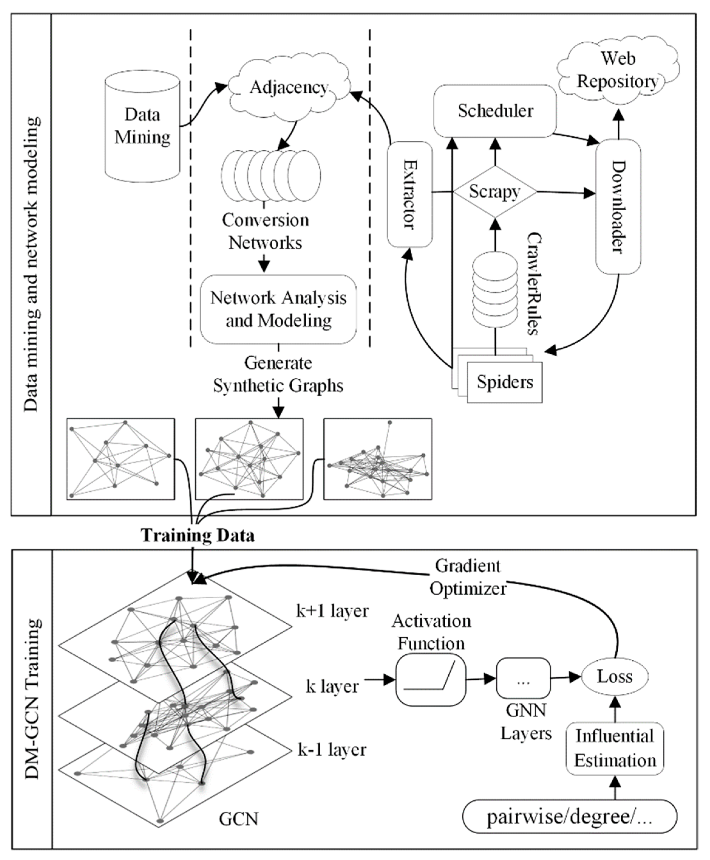
Figure 1, the whole framework of DMGCN consists of two parts.
Table 1 provides the list of notations used in this paper. The first part includes data mining and training data generation. To address the lack of training data, we first collected the training data automatically by data mining and then generated synthetic networks with the same statistical properties as the original data. The great success of deep learning algorithms benefits from the diverse training data sets available; for example, ImageNet in CV, LFW in face recognition, and SquAD [
25] in NLP. The analysis of engineering data, however, always encounters the problem of data scarcity. It is often infeasible to generate massive data by hand as in other fields and the direct use of the collected dataset for training is prone to model overfitting.
Real-world complex systems often share topological and statistical properties, such as being small-world, scale-free, and highly clustering, with generative rules and evolutionary models. DMGCN first detects the type of network by complex network and centralities analysis and then generates numerous synthetic networks with the same characteristics by the corresponding evolution model. Since the evolution model of complex networks is generally simple, we can efficiently generate synthetic networks of different scales to provide sufficient training data for the next step of GCN training.
In the second step of the DMGCN, we trained an identification model of the key nodes from the generated data. Taking the training efficiency and identification accuracy into consideration, we chose GraphSAGE [
17] as the backbone framework. To learn how the information of a node is aggregated by the features of its neighbors, we obtained a representation of a node by combining the features and neighbor relationships of each node. For transductive methods, such as GCN, a unique embedding is learned for each node. In contrast, GraphSAGE generates the node embedding according to its neighbors. GraphSAGE further extends the aggregation method by LSTM (Long Short-Term Memory), Pooling, and other aggregation methods, besides simply averaging. It has the following features: (i) solving the problem of memory explosion by fixed-size neighbor sampling, suitable for large-scale graphs; (ii) transforming transductive learning into inductive learning; and (iii) avoiding retraining the features of nodes each iteration. With incremental features, GraphSAGE can effectively prevent training overfitting and enhance the generalization ability of trained models.
The complex network can be represented through a graph
which is comprises a set of vertices or nodes
and edges
between them. The vertices or nodes may represent actors, co-authors, or data format, while the edges or the links may represent co-starring, co-authorship, or data translation. In addition to the structure of the graph, each vertex has its characteristics
which is usually a high-dimensional vector. The embedding of the central node
in
can be described as:
where
denotes a differentiable aggregator function, such as
,
and
;
denotes functions, such as non-linearity neural layers; and
denotes a neighborhood function. To keep the number of neighbors the same, we filtered neighbors of a node according to the
betweenness centrality and discarded neighbors with smaller
betweenness [
16]. Embedding features of the graph with lower-dimensional data enables better results to be obtained in tasks of graph analysis. By replacing the data of the original graph with graph embedding, the topology of the graph and the correlation among nodes can be preserved. In the GraphSAGE model, the
-layer representation of a node is related to the
layer representation of its neighbors, and this local feature results in the
-layer representation of a node only related to its
network.
To obtain the feature representation of nodes, DMGCN first concatenates transformed self-connections and features of sampled neighbor nodes linearly and then performs ReLU linear transformation. In addition, the neighbors of a node also aggregate the information of their neighbors. Hence, in the -layer aggregation, the node receives the -order information of its neighbors. For graph embedding, we do not take a large recursion and only extend to the second-order neighbors ( = 2). This is reasonable in real life, where friends and family belong to the first-order neighbors. For example, we may hear stories relating colleagues and friends, which have a certain impact on us; these people belong to the second-order neighbors, but further third-order neighbors may not have any influence on us.
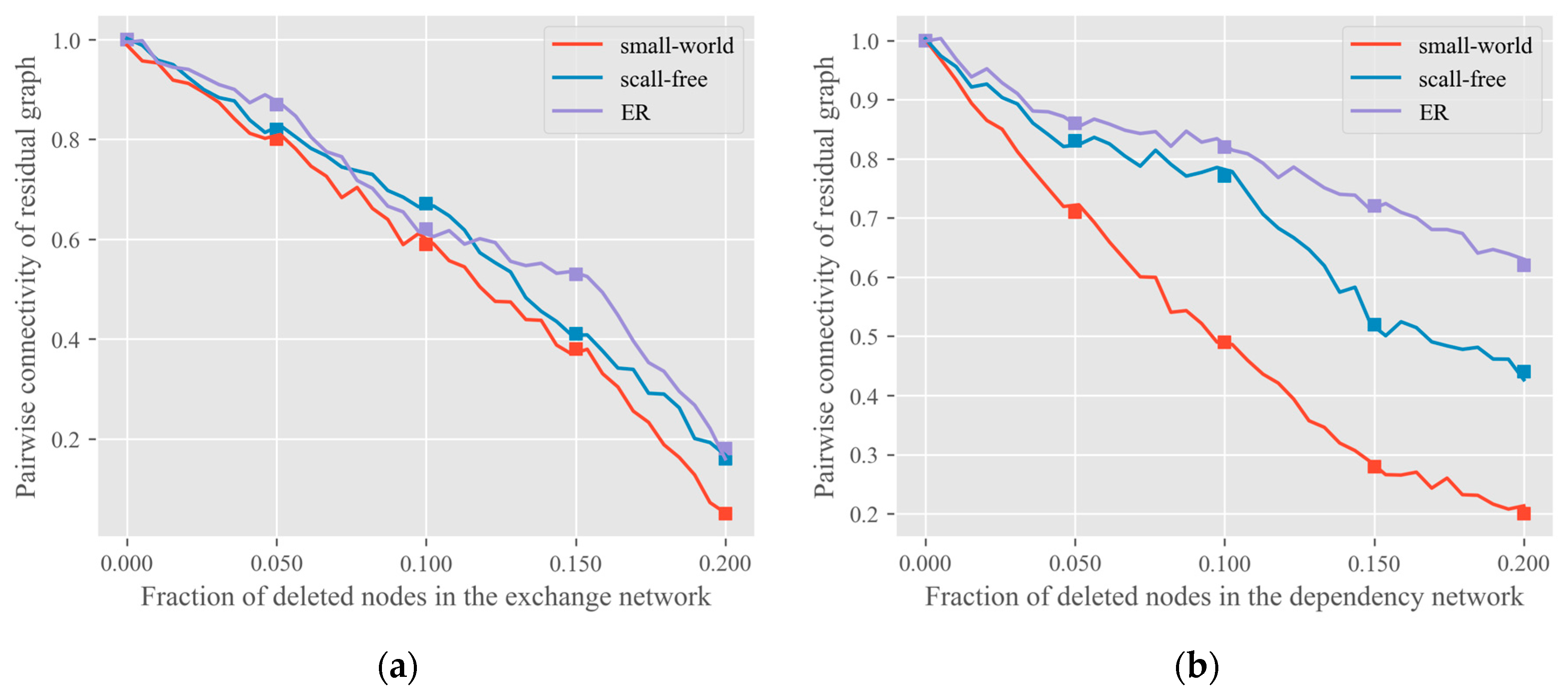
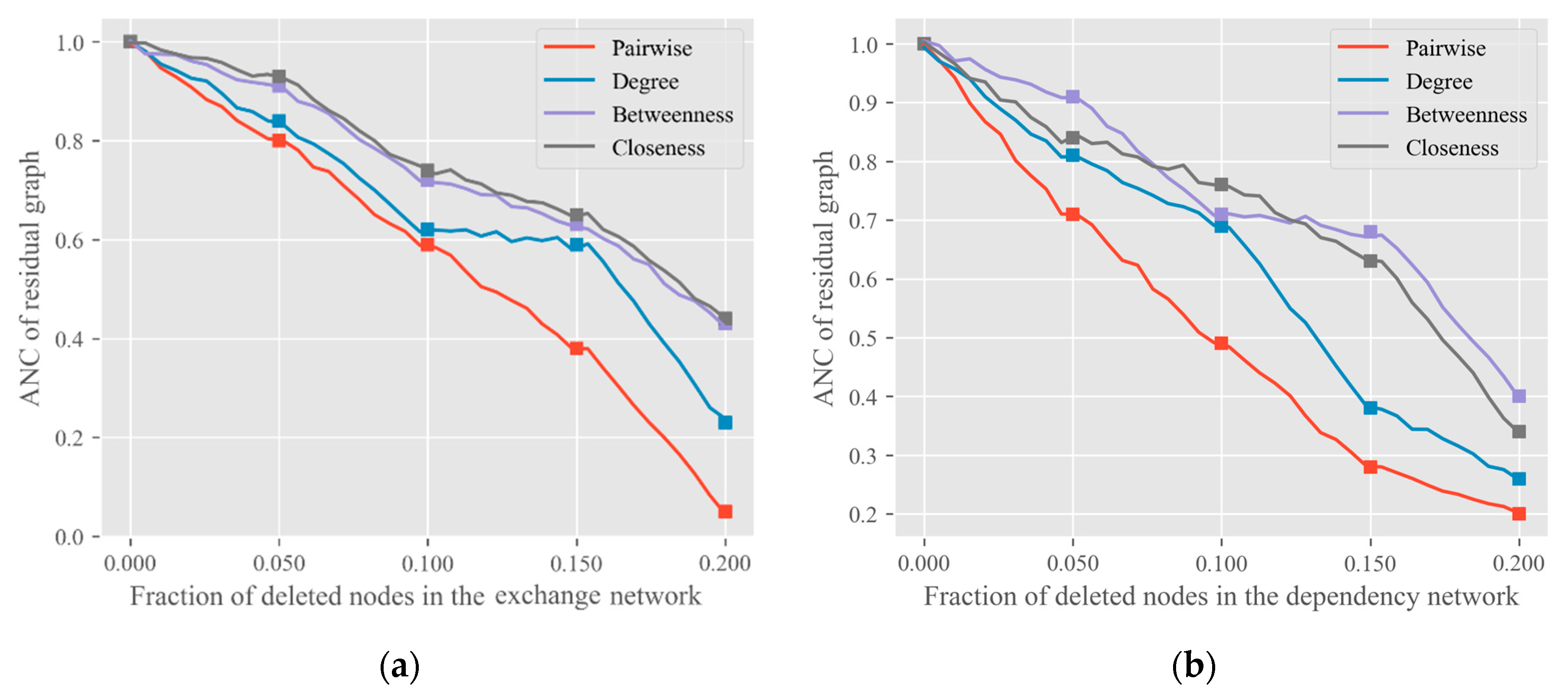
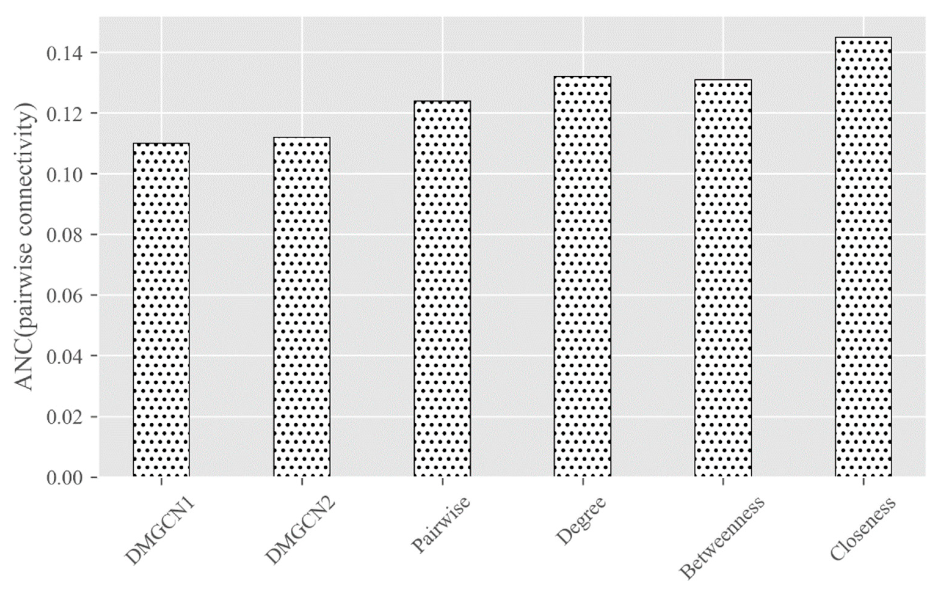
Once completing the encoding of a graph, we will evaluate the change of the graph based on the connectivity measurement. We adopted
ANC (Accumulated Normalized Connectivity) [
10] as the loss function, defined as follows:
where
is the number of nodes in a graph
,
denotes the
-th node in
.
denotes the connectivity of the residual graph after removing the node-set
from
.
is the initial connectivity of
. Any well-defined connectedness measure that translates a graph into a non-negative number may be handled by
ANC. Appraisal of the location of nodes in the network is a problem of node centralities. It is an effective measure to evaluate the performance of individuals, groups, or entire networks. As shown in Equation (2), we use the pairwise connectivity
to measure the critical node, where
is the
-th connected subcomponents in G and
is the size of
. If the
is removed from
, the
ANC of
reduces fastest. We will think that
is the current most important node in
.
The training process of the DMGCN may be slow or even difficult to converge. To alleviate the problem of the non-stationary distribution of training data, previous states can be randomly sampled by using the empirical playback mechanism, so that the training becomes smoother. This technology gathers many rounds into one playback memory. In the inner loop of the algorithm, small-batch updates are applied to the empirical samples randomly sampled from the stored sample pool. Compared with the standard training process, each historical step may be used in multiple weight updates. Secondly, because of the strong correlation between samples, it is easy to over-fit if a batch of quadruplets is taken as the training set directly in sequence. To solve this problem, we can simply randomly select a small number of quadruplets from the experience pool as a batch, which not only ensures that training samples are independent and identically distributed, but also makes the sample size of each batch small, thus speeding up the training speed.
The parameters of this model were tuned by backpropagation and gradient descent methods, commonly used in deep learning. As training proceeded, we gradually obtained a network capable of generating an accurate adjacency matrix and modeling the rules of inter-node connectedness. Finally, we combined it with a graph convolutional network for key node identification.
3.2. Complex Network Measures
To generate synthetic networks with corresponding structural features as real-world networks, a matching evolution model must be selected. The type of networks can be determined based on complexity measures, including the
degree distribution,
clustering coefficient, and so on. These measures are important parameters for the correlation between real networks and synthetic networks [
26].
There are a variety of centrality measures to evaluate the influence of nodes on importance and effectiveness. The
degree of centrality is the simplest way to identify centrality. The
degree of a node
is denoted by the number of all other nodes connected directly to the
and is given by:
where
is the number of nodes in
and
is a binary function, whose value is 1 if
and
are connected, otherwise its value is 0.
Degree portrays the central nodes in a network analysis by the most direct measurement. In scale-free networks, some nodes have very high degrees of connectivity, while most have small degrees.
Evidence shows that in most practical networks and social networks, nodes have a strong tendency to form groups. The
clustering coefficient is another measure on a graph tending to gather together. The local
clustering coefficient gives a single measure of how close its neighbors are to its full connectivity. Given
is the number of all closed triplets (3 edges and 3 vertices), including vertex
in graph
, and
is the number of all open triplets (2 edges and 3 vertices), including
, the
clustering coefficient can be defined as:
A graph is called a small-world network, if it is much larger than the average clustering coefficient of a structure on the same set of vertices of random graphs, and its average path length stays the same as that of the random graph at the same time. In a random network, that is, .
3.3. Case 1: Production Data-Exchange Networks
File formats are commonly used to represent the medium arrangement and layout of electronic documents. With the rapid development of computer and network technologies, an increasing number of documents are being produced and preserved in digital form. In particular, the number of computer-aided design (CAD) file formats remains uncontrolled. Many file formats, such as IGES, STEP, STL, and DXF are considered de facto standards, while new file formats, such as AMF and 3MF, are often created to replace them to adopt emerging technologies, e.g., AM (Additive Manufacturing).
To reduce the laborious work involved in data collection and formulation, automated build of the format exchange network is now a necessary step to ensure product data migration. Web crawlers are used to effectively collect formats and exchange data. Online file formats and software catalogs, such as like
AlternativeTo [
27] and
File-Extensions [
28], provide rich information about thousands of file types and their associated applications. We used
AlternativeTo to collect CAD software tools. The
cad and
3d-modeling tags were selected to find related software. To limit the scale of the exchange network and maintain data fidelity of migration, only exchange tools that exchange vector data were included. In general, less attention is given to software so it sometimes lacks sufficient information for product data migration, thus only software with more than 10 export or import formats were candidates for exchange formats. The
File-Extensions site is the world’s largest computer file extension library, with a detailed explanation of each file type and links to associated software programs; this makes it appropriate for the collection of product data exchange information.
To extract information from sites that do not provide an open API, we adopted the crawler framework, Scrapy. Once the webpage is completely downloaded, Downloader sends the response content to Spiders, which transfers the response to an HTML Filter for further processing. Filter is the key for data mining and extracts the CAD software information from AlternativeTo and feeds them to the File-Extensions site for retrieval of open-and-save and import-and-export format information that the software supports. Due to the asynchronous network, the dependency is first saved in an intermediate file for each CAD system. The process repeats until there are no more requests from Scheduler. We applied RandomUserAgentMiddleware to prevent the crawler from being identified and blocked by web servers because of the default user-agent. When extracting product data information, it was found that the AlternativeTo Service Internet connection was unstable, so ProxyMiddleware was used to process requests using the proxy server.
After all the conversion relationships had been collected, they were converted to a
GraphML file for graph construction and to calculate the measures of the exchange networks. After the extension names of file formats were cleansed, data for about 1673 nodes (data formats) and 10,123 edges (exchange relationships) were finally available for the network.
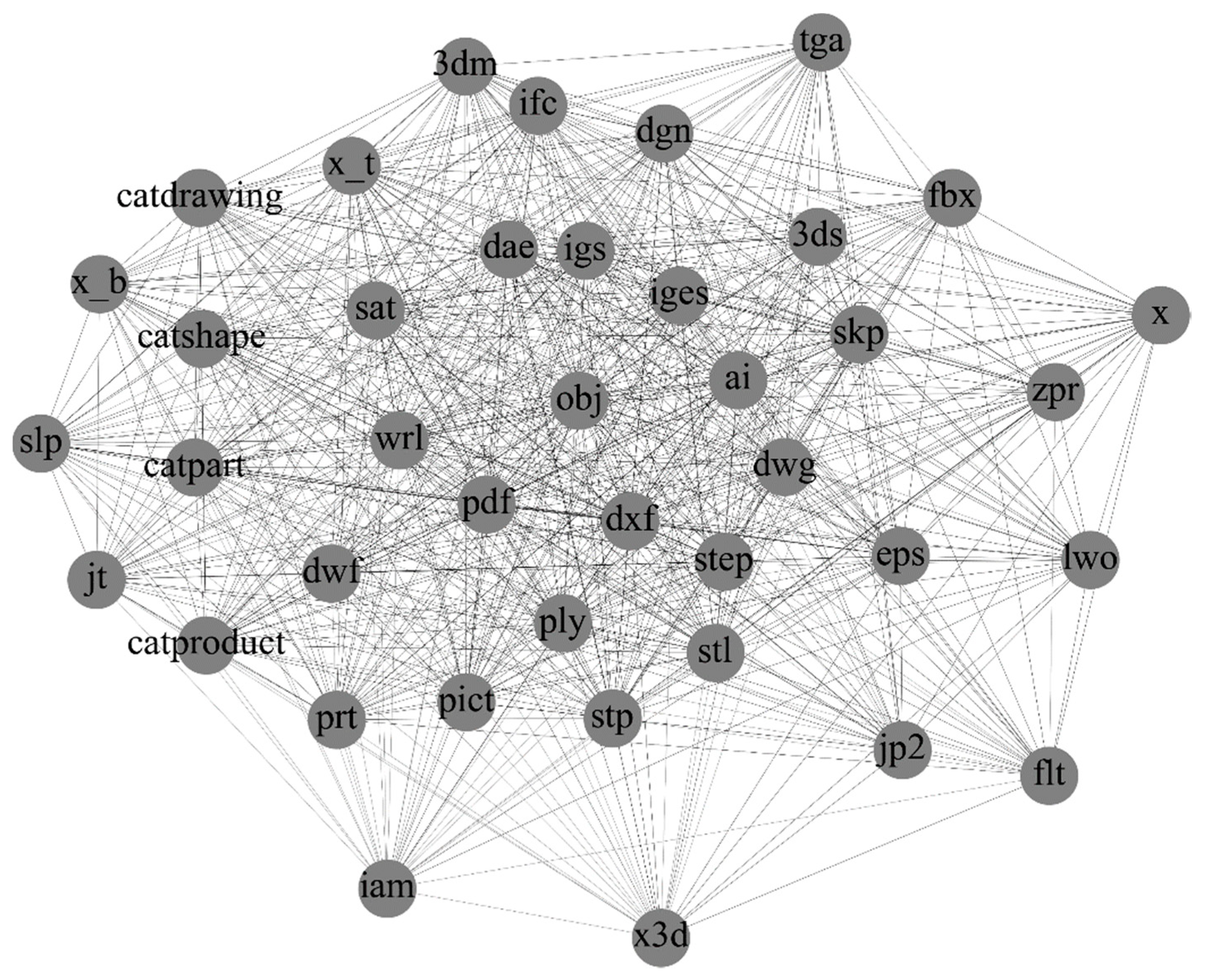
Figure 2 shows the subgraph consisting of 40 nodes with the largest degree of data formats in CAD. It can be seen that popular formats, such as
iges,
dxf, and
stl, have numerous edges and links. Although we cannot guarantee the accuracy of the collected results, the data scale is sufficient to guarantee the reliability of the analysis results.
The metrics of the production data-exchange network are shown in
Table 2. Besides the degree and clustering coefficient, we also measured the Betweenness and Closeness centralities in the production data-exchange network. Betweenness is the number of the shortest paths through a node and describes the bridge importance of a node. Closeness is the reciprocal of the average shortest-path distance to a node. These measures help to determine the importance of a node in a network.
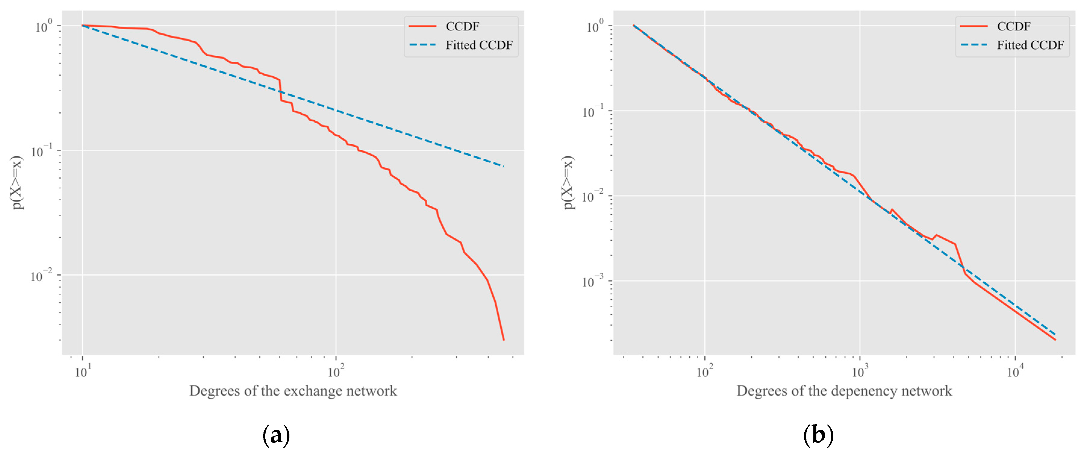
The average degree of the network was about 6.15. The number of edges was 2,797,256 in a complete graph with the same number of nodes, which is more than 276 times greater. Hence, the exchange network is sparse, which is similar to other complex networks. The network diameter was 3, that is, any file format in the network can be converted to another through two translation tools. The result reveals that the population of translation tools for CAD data is very small in terms of the number of data formats.
The clustering coefficient is defined for undirected graphs, so it was necessary to transform our directed graph into undirected. The clustering coefficient of the exchange network was about 0.150, which can be compared with the value coming from network models. For the corresponding Barabasi–Albert (BA) model with the same number of nodes and m = 6, a network with 10,017 edges was obtained, where is the number of new edges in each step. The clustering coefficient of the BA network was 0.306, which is in the same order of magnitude as that of the exchange network. Considering its average path length was 1.92, it could be said that the exchange network is a small-world network, which provides further evidence that complex networks are widespread in the real world.
3.4. Case 2: Operating System Package Dependency Networks
Software systems represent another important field where complex network theory may provide a valuable research method to manage functional complexity and high evolvability. Software systems are the core of the information-based world and hold a position of great importance in modern society. Software comprises many interacting units and subsystems. owever, it is still relatively new and not well-studied in complex networks. A reason for this is that collecting and analyzing data is forbidden or impossible because source code is inaccessible in commercial software. However, the rapid development in the open-source software (OSS) domain now allows researchers to access some software systems and collect data easily. We carried out an empirical network analysis on the package dependency network of the open-source operating systems by modeling packages as nodes, and dependencies among them as edges.
As a software-running environment, the operating system occupies a special place in the open-source software framework. Most Linux distributors now use a program, or set of programs, called a “pre-built package” to install software easily on release. A package is necessary to compile or run an application-bundle-related component. Packages typically include a series of commands to achieve all documents necessary. Since resource reuse is a pillar of the OSS, a package often depends on other packages, which may be toolkits, such as vim, find, and third-party tools, and resource packages, such as images, to work properly. Package dependencies often span across the whole project development group.
To offer a meaningful understanding of evolutionary processes, we analyzed a specific version of the Ubuntu (16.04 LTS) operating system. First, the package data were extracted from the x86_64 branch by the python-apt package. Each vertex is represented by the name of the package. Among a range of dependencies, only
depend and
pre-depend relations were dealt with to represent edges since that is the default behavior of the package management system. The dependency graph was then created through the Python module igraph [
29]. While another Python complex network package, NetworkX [
29], is popular and trivial to use, its performance becomes unacceptable when the graph size increases to tens of thousands of vertices or edges. Last, 20,233 packages that did not exist in the deb packages database were removed. In the deb database, multiple versions of the same package may be specified in the dependency, so 3877 duplicate edges were removed. After the above processing, 47,063 packages and 174,819 directed edges were finally available.
The graph measures are summarized in
Table 3. Each package depends on about four other packages on average. The
clustering coefficient of the dependency network was 0.15. A random network with as many nodes as the package dependency network can obtain a clustering coefficient of 7.89 × 10
−5. That is, the
clustering coefficient of the Ubuntu network is about 1951 times higher than that of the random graph. For the corresponding BA model with the parameters
,
, we obtained a network with 188,921 edges. The
clustering coefficient of the network was 0.0032. The parameters of the two models give a clustering coefficient two orders of magnitude smaller than that of the package dependency network, which is far lower than the random network. It can, therefore, be concluded that the package dependency network is a scale-free network.


