Abstract
With the continuous promotion of urbanization, the generation of construction and demolition waste (CDW) is increasing. The environmental problems and safety hazards caused as a result need to be resolved. In this paper, based on the system dynamics (SD) theory, the modeling, the cost, and the environmental benefit of CDW resource management under the life cycle assessment (LCA) are proposed. Specifically, we propose a combined policy derived through three variables, namely, fines, subsidies, and charges. The target is to reduce illegal dumping behavior and landfill volume and to improve the recycling volume and environmental benefits. The model is constructed with the help of the software VENSIM, and the validity and feasibility of the model are demonstrated with data from Nantong City. The results show that a single policy cannot simultaneously improve environmental benefits, illegal dumping, recycling, and landfill behavior. A combined policy combines the advantages of three single policies, fines, subsidies, and charges, which not only can effectively curb illegal dumping and landfill disposal under the premise of prioritizing environmental benefits, but can also promote the recycling of CDW. The reasonable range for the fine is 300–350 CNY/ton; the rational range for subsidies is 30–40 CNY/ton; and the flexible range for treatment charge is 40–80 CNY/ton. The model can be used for the quantitative assessment of urban CDW management costs and environmental benefits and can also provide a theoretical basis for the government.
1. Introduction
Construction and demolition solid waste (CDW) refers to the muck, waste concrete, waste masonry, waste metal, waste bamboo, wood, and other wastes generated during the construction, demolition, and repair of buildings. With the acceleration of industrialization and urbanization, the construction industry is also developing rapidly, accompanied by an increasing amount of CDW. According to incomplete statistics, the construction industry consumes more than 40% of the Earth’s raw materials on average. At the same time, CDW accounts for more than one-third of the weight of solid waste in the world, and approximately one-third of the total carbon dioxide and greenhouse gas (GHG) emissions [1]. As far as China is concerned, the amount of CDW accounts for more than one-third of the total urban solid waste. More than 300 million tons of CDW are generated every year. If a simple stacking method is adopted, the treatment of new CDW each year accounts for 150 million to 200 million square meters of land. The vast majority of CDW is transported by the construction unit to suburbs or villages for open stacking or landfill without any treatment. This not only consumes a lot of construction funds such as land requisition fees and garbage removal fees but also causes serious environmental pollution due to the scattering of dust and lime sand in the process of removal and stacking. The biggest danger of open-air accumulation is collapse. A case of the rapid and random dumping of solid waste, with no compaction and drainage treatment having occurred, resulted in a fatal landslide in Shenzhen, China. The affected area of this accident was approximately 0.38 km2. It destroyed 33 buildings and killed 77 people [2]. It is a painful fact that this incident was caused by waste accumulation. In addition, there are many polluting materials, such as building components containing carcinogenic asbestos, roof felt containing carcinogenic polycyclic aromatic hydrocarbons (PAH), flame retardants containing persistent organic pollutants (POPs), and so on, which bring great harm to the environment and human beings [3]. Therefore, effective CDW management is essential to minimize the adverse impact of CDW on the environment [4,5].
CDW is not useless. After much experimental research, scholars have developed many recycled building materials, such as recycled concrete blocks and recycled aggregate concrete [6,7], sustainable aviation materials [8], cold asphalt mixture [9], and building heat insulation and sound insulation materials [10]. Vieira and Pereira [11] studied the use of CDW as the base of road infrastructure. They found that it represents an effective measure to achieve social sustainable development. In addition, construction solid waste can also be used for composting with cow dung [12]. Moreover, the recycling of concrete and brick waste can increase its economic value by approximately USD 44.96 million [13].
The rational use of natural resources is one of the basic pillars of sustainable development in modern society. It is necessary to value the waste of the construction industry, which is also a way to achieve sustainability [11]. Recycling CDW based on a circular economy can not only save energy but also reduce GHG emissions, thereby reducing the burden on the environment [14]. The implementation of a waste management plan helps to reduce the dumping of CDW; the larger the scale of the project, the greater the impact of the implementation of the CDW management plan on the benefits [15]. Therefore, promoting recycling is a key measure to alleviate the problem of construction solid waste in China and other places.
2. Literature Review
The development of CDW recycling in many countries is in an early stage. After a long period of exploration, a series of fruitful research results have been achieved. Many scholars have provided detailed discussions on the CDW resource management system from different angles and using different methods. In detail, we can study the CDW resource management system from the aspects of the turnover management system, transportation, site selection for treatment plants, environmental cost, the screening of influencing factors, generation prediction, etc. The CDW turnover management system can improve the efficiency of solid waste treatment and environmental safety in the region [16]. This requires every participant in the construction industry to clarify their goals and responsibilities in the construction solid waste treatment system [17]. Araiza-Aguilar, et al. [18] proposed multi-criteria evaluation technology and a network analysis through GIS technology to determine the best location for CDW treatment infrastructure. The installation of recycling facilities at the construction site saves 64% of the cost of transporting the CDW to the recycling plant for treatment. Transportation cost is an essential factor affecting the cost of CDW treatment [19]. The total transportation cost depends on the transportation kilometers and transportation fee. The cost of recycling solid waste is 72.5% lower than that of a simple landfill. The cost-effectiveness of recycling is 49.5% higher than that of a landfill [20]. Reducing transportation, improving the on-site recovery rate, improving the quality of recycled materials, and maximizing the use of recycled products are the best measures to significantly improve resource efficiency and reduce environmental impact [21,22]. Owing to the complexity of the transportation problem, it is included in this paper as part of future research.
To establish a sound management system, the key influencing factors need to be determined. The main factors affecting the construction of solid waste resource management systems are laws and regulations, government economic incentives, design schemes, classification and sorting technology, and reduction awareness [23,24,25]. In the meantime, predicting and estimating waste generation is critical to waste management. Three main methods are usually used to estimate the generation of CDW: the floor area estimation method, the material flow analysis (MFA) method, and the geographic information system (GIS) method [26]. Next, the quadratic exponential smoothing prediction method, gene expression programming (GEP), gray model, random forest (RF), multivariate regression analysis, artificial neural network, deep learning, and nonlinear autoregressive back propagation (NARBP) neural network model for future years of CDW generation are predicted [27,28,29,30,31,32,33].
To improve the efficiency of the resource-based management of CDW and analyze and reduce the environmental impact and sustainability at large, researchers have used life cycle assessment (LCA), material flow analysis (MFA), geographic information systems (GIS), PESTEL models, and multi-objective mathematical planning decision models [34,35,36,37]. Quantitative and qualitative data serve as a basis to help decision-makers manage and plan for CDW [38]. Thongkamsuk, et al. [39] set collection, transportation, and disposal fees as a strategy to encourage Thai entrepreneurs to segregate their CDW. Increasing recycling rates and reducing landfill rates for CDW not only increase the potential economic value of recycling but also significantly reduce land use and potential environmental impacts [40].
As an indispensable part of pollution prevention and control, solid waste environmental management is inseparably related to air, water, and soil pollution prevention and control, and runs through the whole process of solid waste generation, collection, storage, transportation, utilization, and disposal, which is related to producers, consumers, recyclers, utilizers, disposers, and other interested parties, and requires collaborative governance among the government, enterprises, and the public. At present, China’s CDW resource management system is still in its initial stage. It lacks a comprehensive accounting of the management costs and environmental benefits of CDW disposal programs. The process of CDW management in China is generally characterized by low waste landfill charges and high management costs, a lack of effective incentives to stimulate recycling enthusiasm, and many other problems. Most importantly, the current state does not quantify the three aspects of fines, subsidies, and waste disposal charges in an integrated manner. The government does not have a clear management plan to reflect the integrated disposal of the three influencing factors. This will result in companies not knowing how to cooperate with the government’s management, and the government having difficulty in managing CDW resources. Many developed countries have set the valorization of CDW as one of the key policy elements supported by the state and have made certain preferential policies in terms of scientific research, emission reduction, fee collection, and economic compensation. Legislation and incentives are effective drivers of green building development [41]. Local governments should develop policies that increase the profitability of practitioners, and not just increase their intentions or regulate waste management [42].
Therefore, this paper intends to draw on the experience of developed countries and establish a compensation model for management costs and environmental benefits by analyzing the current situation of CDW resourceization in China. The main objective of this paper is to propose new management approaches and quantify specific rewards and penalties to achieve better management results. Through the comprehensive analysis of management costs and environmental benefits, the management costs of CDW under different management methods can be clarified. Thus, a reasonable method for reducing the cost of CDW can be established, providing a theoretical basis for the government. Section 3 describes the specific modeling process. Section 4 demonstrates the applicability of the proposed model through a case study in China. Section 5 discusses the model’s strengths and weaknesses and future research directions. Finally, in Section 6, the main conclusions of the paper are given.
3. Materials and Methods
3.1. System Dynamics
The method of system dynamics (SD) was first proposed by Forrester [43]. It is a method used to deal with the dynamic behavior of information feedback systems. It allows a quantitative description of nonlinear, higher-order, and dynamic complex systems through computer simulations [44,45]. Causal loop diagrams and stock flow diagrams are commonly used to reflect the systematic relationships among variables. Assigning equation relationships to the variables can transform a qualitative problem into a quantitative one. System flow diagrams are mainly composed of stock, auxiliary variables, constants, flows, and shadow variables.
Many researchers have conducted in-depth studies on system dynamics approaches. Wu, et al. [46] developed a system dynamics model of work conflict among employees in the construction industry. The simulation results showed that the level of work interference and family conflict (WIFC) experienced by employees in the construction industry was significantly greater than the level of family–work conflict (FIWC). To successfully evaluate the investment related to integrated information management in the construction industry, a qualitative system dynamics model was depicted using causal loop diagrams for studying the dynamics of a construction enterprise resource planning system (C-ERP) [47]. Liu, et al. [48] constructed a system dynamics model to explore the dynamic relationship of process safety culture in the Chinese chemical industry and to study the stakeholder dynamic stability. Thirupathi, et al. [49] developed a suitable system dynamics model to identify the factors affecting sustainable initiatives and appropriate performance indicators in an automotive parts manufacturing organization. A system dynamics model called industry-effects-policy-system dynamics (IEP-SD) was designed to analyze the environmental and economic impacts of eco-industrial systems by simulating long-term trends, centering on Huinong, a typical coal city in western China [50]. This showed that the system dynamics model can be used to analyze and capture the main influences. Most importantly, the SD model can simulate trends in the system under different policy scenarios to determine the most effective policy measures [51]. The reasons for choosing the system dynamics model in this paper are as follows:
- (a)
- CDW resource treatment is inherently a dynamic system based on time variation, which is fully consistent with the premise of using system dynamics models.
- (b)
- The structure of the construction waste resource treatment system contains various types of variables, such as “flow”, “rate”, “auxiliary “, and “product level (level)”, which facilitate modeling.
- (c)
- The SD model can be simulated and analyzed to arrive at a reasonable range of values, and dynamic simulations can be conducted to vividly identify the trend of each product in the simulation process; then, the environmental and economic impact of the CDW system can be analyzed.
3.1.1. Causal Relationship Diagram
Assessing the long-term economic and environmental impacts of key variables on CDW management programs is possible with a tool for visualizing variable relationships and system feedback effects, namely the SD model. The causal loop diagram of SD is the general idea of the whole model and is a qualitative representation of the model. The causal loop diagram is drawn by VENSIM software. To present more intuitively the logical relationship between the model as a whole and between variables, the causal loop diagram of management costs and environmental benefits is further developed based on the analysis of the model boundaries and the constituent elements. Usually, causal loop diagrams are conceptual models that can portray causal links between variables, effectively depicting the nature of the links between things in the system and reflecting the causal relationships that exist in complex systems. When the causal chain of two or more variables forms a closed loop, then this causal loop can be called a feedback loop.
The causal loop relationship between CDW generation and the disposal subsystem is shown in Figure 1. There are eight loops in Figure 1: R1, R2, R3, R4, R5, R6, R7, and R8. The use of arrow line diagrams with directional markers reflects the causal relationship between variables. There is a relationship of influence points from the acting variable to the location of the variable being acted upon. If two variables have a positive effect relationship, the causal relationship is indicated by a “+”, i.e., the previous variable can positively contribute to the next variable. If two variables have a negative inhibitory effect, the causal relationship is indicated by “−”, i.e., the previous variable has an inhibitory effect on the next variable. The colors are used to distinguish the different circuit paths: orange represents loop R1, cyan represents loop R2, pink represents loop R3, green represents loop R5, brown represents loop R7, red represents loop R8, and navy represents loop R10. Note in particular that R4, R6, and R9 are each made up of existing colors. The base color of the arrows for the rest of the picture is blue.
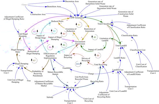
Figure 1.
Causal relationship between CDW generation and disposal subsystem.
Feedback loops R1 and R2 mainly reflect the effect of government regulation on the amount of solid waste generated. The huge amount of solid waste generation has attracted the attention of the government; so, the government has increased its regulatory efforts. The government’s regulatory efforts can be realized in two ways. On the one hand, they raise people’s awareness of reduction through publicity and education. This can inhibit the generation of CDW from the perspective of human behavior. On the other hand, enterprises must reduce the generation of solid waste by improving laws and regulations. Laws and regulations usually act in the design and planning stage. In the whole life cycle, the design and planning stage is both the source of CDW generation and the end of its treatment [25]. Initially, reasonable design planning can effectively avoid an excessive production of CDW. Then, the generated CDW can become recycled products through resource treatment. The application of recycled products in new buildings requires the help of design and planning stages. For example, after the feasibility study stage, the design unit should specify the parts of recycled products, the minimum application ratio, and the technical index in the construction drawing design documents. Such a cycle is the embodiment of the resourceful recycling of CDW.
Feedback loops R3 and R4 partially overlap with R1 and R2, respectively. They mainly reflect the influence of the total amount of illegal dumping on the government’s regulatory efforts. The amount of illegal dumping is a part of the amount of solid waste generated. The impact of sinking accidents [2] and environmental pollution caused by illegal dumping is huge. The greater the total amount of illegal dumping, the greater the safety impact and amount of environmental pollution generated. This shows that the total amount of illegal dumping can increase the level of government regulation. Feedback loop R7 indicates the influence of laws and regulations on illegal dumping behavior. The improvement and enforcement of regulations can greatly increase the chances of punishment. When the cost of violating regulations increases, illegal dumping behavior will naturally decrease.
Feedback loops R5 and R6, like R3 and R4, contain overlapping paths. They mainly reflect the impact of the total amount of landfilled CDW on the government’s regulatory efforts. Similarly, the greater the volume of solid waste landfilled, the greater the impact on the loss of land resources and environmental pollution. This will increase government regulation and promote the resource treatment of CDW, thus reducing the impact on the ecological environment.
Similarly, feedback loops R8 and R9 demonstrate the effect of total solid waste recycling on the intensity of government regulation. Finally, feedback loop R10 describes the positive contribution of government regulation to the total amount of solid waste recycling. Well-established laws and regulations can regulate the market system. Thus, recycling costs are reduced to promote recycling behavior. Overall, the government plays a regulatory and promotional role in the whole system. The government’s actions are a major factor in promoting the resource utilization of CDW.
Environmental benefits refer to the corresponding changes in the structure and function of the environmental system caused by the emission of pollutants and environmental management under the condition that the enterprise occupies and consumes certain natural resources, thus causing effects on production and the living environment. In simple terms, if the same natural resources are occupied and consumed, the environmental benefits are good, if the ecological balance can be maintained and the production and living environment of the enterprise and the surrounding residents do not deteriorate or improve; on the contrary, if the environmental and ecological balance is broken and quality of life and the environment deteriorate, the environmental benefits are poor. Environmental benefits mainly include those derived from the reduction in energy consumption, solid waste landfill, GHG and the illegal dumping of solid waste, and the recycling. Assuming that the environmental costs saved are equal to the environmental benefits, the subsystem of environmental benefits of construction solid waste can be represented by Figure 2.
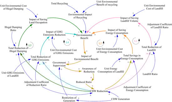
Figure 2.
Causal relationship of environmental benefit subsystem.
Figure 2 shows the causal loop diagram of the environmental benefit subsystem of CDW. Pink represents loop L1, orange represents loop L2, cyan represents loop L3, and green represents loop L4. These loops clearly indicate that the total volume of solid waste landfill savings, total savings in energy consumption, the reduction in illegal dumping, and the total reduction in greenhouse gas emissions all contribute positively to the environmental benefits. The reduction in solid waste generation not only reduces the area of land occupied by illegal dumping, the area of land occupied by landfill disposal, and the total greenhouse gas emissions, but also saves energy consumption. The greater the environmental benefits, the greater the level of government regulation. Thus, people’s awareness of reduction can be improved, which will ultimately reduce the generation of CDW.
3.1.2. Stock and Flow Diagram
Stock and flow diagrams are a refinement of the idea, assigning quantitative values to linear or non-linear relationships between variables through equations and parameters, in order to transform them from a qualitative to a quantitative model. Stock is the cumulative quantity, characterizing the state of the system. Flows are rate quantities, characterizing the rate of stock change. The evolution of stocks is caused by flows only. Most importantly, the stock–flow perspective represents continuous time. The mathematical meaning of the stock is integral, as expressed in Equation (1). The flow is the net rate of change of the stock, that is, the derivative of the stock. It can be expressed by differential Equation (2).
Since total transport costs depend on the number of transport kilometers and transport fee [20], it is not possible to simply rely on specific data for the analysis. This paper assumes that the transportation cost is 0. Due to the complex and variable nature of transportation costs, this area will be a focus of future research. Therefore, the research environment in this paper is set up without the influence of transportation. According to the causal loop diagram, the cost–environmental benefit model of construction solid waste resource management is drawn, as shown in Figure 3.
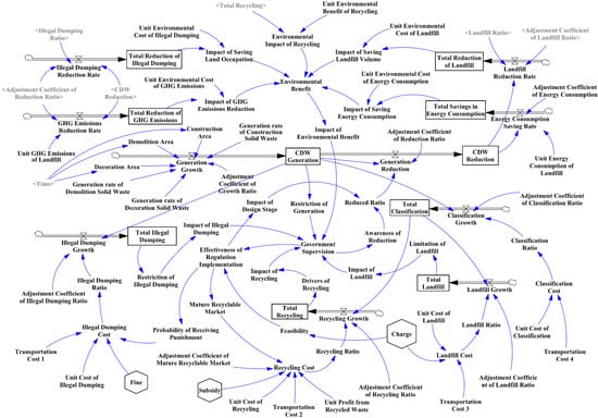
Figure 3.
Environmental benefit stock flow chart of CDW resource management. The hexagon indicates the independent variables to be analyzed in this model. The rectangle denotes the stock. The double-linear arrows represent the rate variables. Those with brackets belong to the shadow variables.
First, it is clear from Figure 3 that the variables of CDW generation, total illegal dumping, total classification, total landfill, and total recycling are stocks. The stock can minimize the change process of the data and is also the focus of analysis in this paper. Secondly, achieving the total amount of illegal dumping, the minimum amount of landfill, and the maximum environmental benefit is an important goal of the model. Under this objective planning approach, fines, subsidies, and charges are independent variables, and each stock and the environmental benefits are dependent variables. In simple terms, by changing the values of fines, subsidies, and charges, we finally achieve the multiple objectives of minimizing the total amount of illegal dumping, minimizing the total amount of landfill, and maximizing the environmental benefits. A simulation analysis is used to determine the reasonable range of fines, subsidies, and charges to achieve this goal. After determining the range of values, the government can use this as the basis for reasonable planning, thus facilitating the process of resource utilization for construction solid waste. The main objectives are as follows: (1) to quantify the environmental benefits; (2) to develop multi-objective planning by adjusting variables to achieve optimal results; and (3) to provide a basis for decision-making and help the government to develop plans.
3.2. Multi-Objective Programming
The hierarchical sequence method is a simple method for solving multi-objective programming. That is, the objectives are given a sequence according to their importance, and each time, the next objective optimal solution is found within the previous objective optimal solution set until a common optimal solution is found. First, the objectives are ranked according to their importance. The priority of the objectives in this paper is environmental benefits, total illegal dumping, and total landfill. That is, the optimal solution set of environmental benefits is sought under the optimal solution set that minimizes the total amount of illegal dumping, and then this is used to find the optimal solution set that minimizes the total amount of landfill. The main process is given in Equations (3)–(5).
where indicate the environmental benefits, the total illegal dumping, and the total landfill, respectively. denote fines, subsidies, and charges, respectively.
3.3. Data Sources
3.3.1. Estimation of the CDW Generation
CDW generation is usually estimated by employing the waste generation rate method, MFA method, building information modeling (BIM), and mixed integer linear programming model. As the name implies, the waste generation rate method calculates the amount of solid waste generated per unit area and then multiplies the result by the floor area to obtain the total amount generated [52]. The MFA method focuses on predicting solid waste generation based on various historical construction material consumption data and estimates of the average service life of materials [53]. BIM is a method that can generate and manage all of the information needed for a building’s life cycle, from design to demolition [54]. Based on the correlation analysis between demolition solid waste estimation and indicators such as population density, the aging index of the building, building density, and land occupation type, a mixed integer linear programming recovery relationship for demolition waste production in a specific region can be established [55]. Zhang, et al. [56] examined and compared the application of three commonly used CDW estimation methods, including the weight per floor area method (WAM), the floor area method, and the weight per capita method. Studies have shown that the weight per building area method is more appropriate due to the availability and accuracy of data at the city or national level in China. Solid waste generation rates usually vary from region to region and from building system to building system due to differences in economic development, city size, building type, construction practices, site management level, and measurement methods. Therefore, researchers usually use the floor area method to quantify the CDW generation rate. The details can be seen in Table 1.

Table 1.
The generation rate of CDW in the literature.
As can be seen from Table 1, CDW includes the amount generated from new building construction, the amount generated from the demolition of old buildings, and the amount generated by building decoration. In the literature, the CDW generated from new construction ranges from 0.018 to 0.099 t/m2 with a mean value of 0.059 t/m2; the amount of demolition solid waste ranges from 0.401 to 1.615 t/m2 with a mean value of 1.008 t/m2; and the amount of decoration solid waste ranges from 0.019 to 0.191 t/m2 with a mean value of 0.105 t/m2. The amount of demolition solid waste is approximately 17 times that of the value given by new construction data. China usually uses weight to express the amount of solid waste; therefore, this paper selects the weight per floor area method and takes the average value in Table 1 as the CDW generation rate.
Without considering the use of the building and the type of structure, this study simply estimates the amount of CDW generated based on the floor area only. The building demolition area can be calculated at 10% of the current year’s floor area [66]. The decoration area is taken as the sales floor area of commercial houses. Therefore, the formula for estimating the amount of CDW generation is as follows.
where is the total CDW generation in a region (unit: t); and are the construction area, demolition area, and decoration area of new buildings in the region (unit: m2), respectively; and , and are the waste generation rates of the corresponding construction types (unit: t/m2).
3.3.2. Variable Equations and Parameter Settings in the Model
The assignment of variables in the model is the focus of this paper. The variables are divided into four main types: horizontal variables, rate variables, auxiliary variables, and constants. Horizontal variables, also known as stocks, describe the effect of a variable that gradually accumulates as time advances. The mathematical definition of a horizontal variable is the accumulation or integral connecting its flow. It is generally represented by a box in the model. Stocks change and accumulate over time. System dynamics can constantly depict and operate on changing system variables. The rate variable, also known as the flow rate, is the magnitude of the velocity of the flow in the system and is divided into the inflow rate and outflow rate. It is generally represented in models in the shape of an hourglass. The mathematical definition of the rate variable is the amount of inflow minus outflow per unit of time. Auxiliary variables are intermediate variables; if the state of factors in the system is subject to the coupling between multiple variables, auxiliary variables need to be added here for description. Constants are the fixed quantities of the auxiliary variables, which are the basis of the model. The variables in the model are often related to more than one variable and are often nonlinear. In this case, a regression analysis, SD-GM estimation [67], table functions, and various logistic functions in VENSIM software are usually used for description.
Constants are usually obtained from official statistics such as statistical yearbooks, historical data, and references. For example, Wang, et al. [68] used the life cycle assessment and willingness to pay methods to investigate the environmental impact of recycling 1 t of demolition waste in Shenzhen. The findings indicate that direct landfilling leads to an environmental cost of 12.04 CNY/t. Therefore, this model can take the environmental cost per unit of landfilled solid waste as 12.04 CNY/t. The adjustment factor of the proportion can be initially set to 1 in 1/year [67]. The constants need to be valued according to the actual situation. Generally, the initial value is taken as 0 or the value of the initial year. The rate variable is one of the auxiliary variables. Except for the constants, the rest of the variables need equations to assign explanatory values. See Appendix A for a detailed description of the variables.
4. Results
The useful life of a solid waste treatment or disposal facility is usually 20 to 30 years [69]. Therefore, the time range of the model can be set to 20 years. Initially, the simulation time was set from 2010 to 2030. The step size was one year. The magnitudes of three variables, fines, subsidies, and charges were adjusted, and then the relationship between their changes in CDW management costs was investigated. This paper takes Nantong City as an example for a simulation analysis.
4.1. Basic Parameter Settings
The new construction floor area and renovation area from 2010 to 2021 can be derived from the existing data of the NARBP model. This model integrates the order recognition capability of the linear autoregressive model and the nonlinear processing capability of the neural network model, and has a high prediction accuracy, with this being widely used in the prediction of generation [33]. The values for 2022 to 2030 were predicted by the NARBP model. The relative percentage errors of the forecast values were verified to be 1.5% and 3.8%. This indicates that the predicted values are relatively accurate and sufficient to serve as the base data for this model. Next, the total construction solid waste in 2010 was calculated based on the floor area estimation method. Based on the current status of construction solid waste management, the initial ratios of 0.03, 0.13, and 0.84 were derived as the initial values of illegal dumping, recycling, and landfill, respectively, in 2010. Therefore, the values of the stock in the model are taken as shown in Appendix A.
4.2. Model Test
Tests are required to demonstrate the reliability and applicability of the constructed model before it can be used formally. Therefore, before running the construction waste management cost simulation model, the model is tested for intuitiveness, sensitivity, and performance under extreme conditions.
- (1)
- Intuitiveness test
The initial inspection of the model is performed using the inspection function that comes with the VENSIM software. The first step is to check the system structure of the model. If the model passes the test, the next step is to check the units of the variables; if the system structure does not pass the test, the model needs to be modified according to the instructions until it passes the test. When the model system structure and unit scale both pass the test, it means that the model can pass the intuitiveness test.
- (2)
- Sensitivity test
Sensitivity testing is when the value of a variable is continuously adjusted to see if the model is an influence and if the model changes within a reasonable range. If the test passes, the model passes the sensitivity test. In this paper, the landfill proportion adjustment factor is selected as the test variable. The normal range of the landfill proportion adjustment factor for construction solid waste is known to be [0, 1]. The coefficients are divided into equal parts and assigned to 0 (Case 1), 0.25 (Case 2), 0.5 (Case 3), 0.75 (Case 4), and 1 (Case 5), and then simulated to compare the changes in the total amount of solid waste landfilled. The specific results are shown in Figure 4.
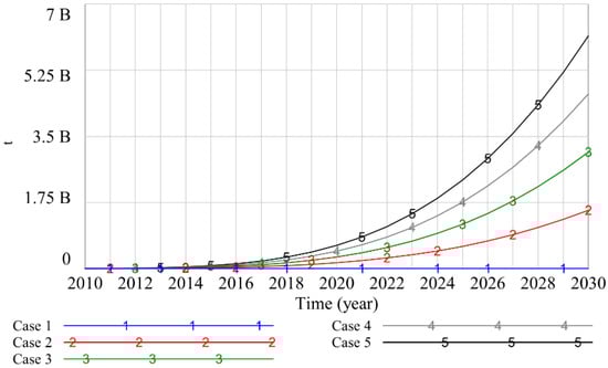
Figure 4.
Variation in the landfill ratio adjustment coefficient.
As shown in Figure 4, when the landfill proportion adjustment factor varies uniformly in the range of [0, 1], the total amount of landfill not only shows an increasing trend with time variation but also increases with the increase in the landfill ratio adjustment factor. When the adjustment coefficient of the recycling ratio is 0, the total amount of the landfill is the lowest; when the adjustment coefficient of the landfill ratio is 1, the total amount of the landfill is the highest. This phenomenon is consistent with objective practical law. At the same time, the graphical change trend remains consistent and does not present overly sensitive or overly insensitive places.
- (3)
- Extreme conditions test
The applicability of the model under extreme conditions is defined as adjusting the initial value of a variable to an extreme situation and observing whether the model results match reality [69]. In this study, an analysis is undertaken to compare the two extreme states of fines and the normal state of total illegal dumping to determine whether the applicability of the model conforms to reality. The variables are set as 0 (F = 0), 100 (F = 100), 250 (F = 250), 350 (F = 350), 450 (F = 450), and 1000 (F = 1000), respectively. The results of the influence of the total amount of illegal dumping of solid waste with the variation in fines are shown in Figure 5.
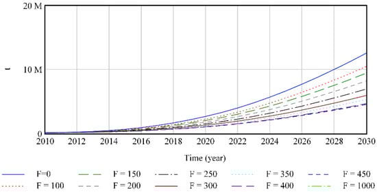
Figure 5.
Impact of fines on total illegal dumping.
From Figure 5, it can be seen that the total amount of illegal dumping tends to decrease when the fine is appropriately increased. This indicates that increasing the fine can effectively curb illegal dumping behavior. When the fine is 0, the total amount of illegal dumping is the largest; when the fine is 1000, the total amount of illegal dumping is the smallest. This is consistent with the objective reality and satisfies the extreme condition test.
4.3. Policy Analysis
In this paper, using fines, subsidies, and charges as independent variables, we intend to derive through the model the optimal results of reducing the total amount of illegal dumping and the total amount of the landfill, and increasing the amount of recycling and environmental benefits.
4.3.1. Fines Policy
By adjusting the value of the fine, the effects on the amount of solid waste generated, sorted, illegally dumped, recycled, and landfilled, and on the environmental benefits, are derived. From Figure 5, it can be seen that the same effect is achieved when the fine is 450 or 1000; therefore, the upper limit of the initial fine should be 450 CNY/t. The range of the fine is (0,450), and the detailed values are 0 (F = 0), 150 (F = 150), 300 (F = 300), 350 (F = 350), 400 (F = 400), and 450 (F = 450). The results of the effect of the fine policy on the main variables are shown in Figure 6. The changes in the total amount of illegal dumping corresponding to different fines are shown in Table 2.
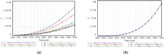
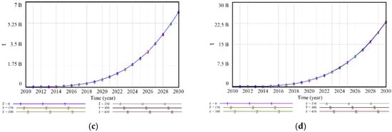
Figure 6.
Effect of fine policy on key variables. (a) Total illegal dumping. (b) Total recycling. (c) Total landfill. (d) Environmental benefit.
Table 2.
Changes in the total amount of illegal dumping corresponding to different fines.
From Figure 6a and Table 2, it can be seen that when the fines change from 0 to 300, the amount of illegal dumping changes from 12,542,400 t to 5,931,770 t: a decrease of 52.71%. This indicates that the fine set at 300 can effectively curb illegal dumping behavior. When the fines reach 350 and 400, the change is small, and the illegal dumping amount is 5,300,640 t and 4,669,410 t, representing a decrease of 57.74% and 62.77%, respectively. The overall rate of change shows a pattern of increasing and then decreasing. From Figure 6b–d, it can be seen that the changes in fines have little effect on the total amount of recycling, the total amount of landfill, and environmental benefits. Combining the actual effects of fines on total illegal dumping, total recycling, total landfill, and environmental benefits in Figure 5 and Figure 6, the reasonable range of fines should be set between 300 and 350 CNY/t.
4.3.2. Subsidy Policy
Wang, et al. [70] introduced four subsidy policies—initial subsidy, recycling subsidy, research and development (R&D) subsidy, and production subsidy—and developed a system dynamics model to explore the impact of subsidy policies on the development of the recycling remanufacturing industry in China. The results show that different subsidies have different incentive goals and characteristics. It is easy to see that a single fine policy only has some impact on the total amount of illegal dumping. Financial incentives are also the most critical driver for the proper management of CDW [25]. Government subsidies not only increase the total profit of the CDW resource utilization supply chain but also enhance the reuse of CDW [71]. A subsidy policy is also needed to control the total amount of recycling. The initial set of subsidies takes a range of values of (0, 100). It can be set to 0 (S = 0), 10 (S = 10), 20 (S = 20), 30 (S = 30), 40 (S = 40), or 100 (S = 100). The effect of different subsidies on the amount of recycling is shown in Figure 7.
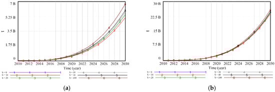
Figure 7.
Effect of different subsidies on the amount of recycling. (a) Total recycling. (b) Environmental benefit.
From Figure 7, it can be seen that the amount of recycling and environmental benefit increase during the increase in subsidy. However, when the subsidy reaches 40 CNY/t, the effect on the recycling volume is smaller, and the change rate is 3.31%, which is less than 5%. Therefore, the upper limit of the subsidy should be set at 40 CNY/t. From Figure 7b, it can be seen that the change in subsidy has less impact on the environmental benefits. From Table 3, it can be seen that as the subsidy increases, the rate of increase in recycling shows a decreasing and then increasing trend. When the subsidy is 40 CNY/t, the cumulative rate of increase reaches 30.87%. Therefore, the most appropriate range for the subsidy is 30–40 CNY/t.
Table 3.
Changes in total recovery corresponding to different subsidies.
4.3.3. Charge Policy
Similarly, controlling the total amount of landfill also requires a solid waste disposal charging policy. The range of values for the initial charge is (0, 1000). The simulation takes the values of 0 (C = 0), 40 (C = 40), 80 (C = 80), 120 (C = 120), 160 (C = 160), 200 (C = 200), 240 (C = 240), and 1000 (C = 1000). The effects of different charges on the main variables are shown in Figure 8. The effects of different charging policies on the total amount of solid waste landfilled and the environmental benefits are shown in Table 4.
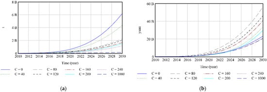
Figure 8.
Impact of different charges. (a) Total landfill. (b) Environmental benefit.
Table 4.
The impact of different charging policies on the total amount of solid waste landfilling and environmental benefits.
It can be seen from Figure 8 that the charge range of 0–80 CNY/t has a large impact on the variation in the total landfill volume, whereas the range of 80–240 CNY/t has a small impact on the total landfill volume. Meanwhile, the environmental benefit reaches its maximum when the charge is 80 CNY/t. When the charge reaches 1000 CNY/t, the environmental benefit reaches its lowest value. From Table 4, we can see in detail that when the charge is 40 CNY/t, the rate of reduction in total landfill is 29.64%, and the rate of the increase in environmental benefit is 45.17%. When the charge is greater than 80 CNY/t, although the total amount of landfill is gradually decreasing, the environmental benefit is also gradually decreasing, and the rate of decrease is faster. Considering that the total amount of landfill is reduced by as much as possible under the condition of maximizing the environmental benefits, the charge range should be set at 40–80 CNY/t.
4.3.4. Portfolio Policy
The literature shows that a combination of policies can combine the advantages of a single policy and thus have a better performance. From the previous section, it can be seen that the optimal ranges of values for fines, subsidies, and charges are (300, 350), (30, 40), and (40, 80), respectively. This finding is close to the results presented in the literature [67], with a range for fines of (300, 400) and charges of (70, 90), indicating that the simulation results are plausible.
Next, this chapter sets up nine policies for the simulation analysis according to the range of values taken. The value ranges of fines, subsidies, and charges are taken as the lower and upper limit, respectively, and then a combined analysis is conducted to analyze the effects on the total amount of illegal dumping, the total amount of recycling, the total amount of landfill, and environmental benefits. The simulation results are shown in Figure 9. The results obtained from the combined policy are shown in Table 5.
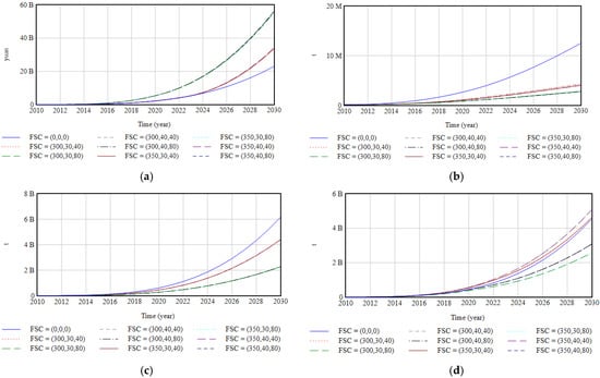
Figure 9.
Portfolio policy analysis. (a) Environmental benefit. (b) Total illegal dumping. (c) Total landfill. (d) Total Recycling.
Table 5.
The impact of portfolio policy on major variables.
From Figure 9, it is obvious that the combined policy not only significantly reduces the total amount of illegal dumping and the total amount of landfill, but also significantly increases the total amount of recycling and the environmental benefits. By combining Figure 9 and Table 5, it can be concluded that the combined policy can reduce the total amount of illegal dumping and the total amount of landfill by 65.55–78.10% and 28.58–63.13%, respectively, and increase the total amount of recycling and environmental benefits by 1.95–12.11% and 45.97–143.86%. These findings fully demonstrate the superiority of the combined policy. In detail, Figure 9a indicates the optimal environmental benefits under the policies FSC = (300, 40, 80), FSC = (350, 30, 80), FSC = (300, 40, 40), and FSC = (350, 40, 80), which are 1.62–2.44 times higher than the other policies. The advantages of these four policies are obvious. Figure 9b demonstrates that the total amount of illegal dumping under the FSC = (350, 40, 80) policy is the least, while the difference between the total amount of illegal dumping generated under the FSC = (300, 40, 80), FSC = (350, 30, 80), and FSC = (300, 30, 80) policies is only 2.62%. This demonstrates that all four policies are conducive to curbing illegal dumping. Figure 9c indicates that the total amount of landfill under FSC = (350, 30, 80), FSC = (300, 40, 80), FSC = (300, 30, 80), and FSC = (350, 40, 80) policies is the smallest. Figure 9d denotes the maximum total amount of recycling under the FSC = (350, 30, 80) and FSC = (300, 30, 40) policies.
According to the multi-objective programming, firstly, the solution sets that satisfy the highest environmental benefits are FSC = (300, 40, 80), and FSC = (350, 40, 80). Then, under this solution set, there is one and only one solution that permits the lowest total amount of illegal dumping, which is FSC = (350, 40, 80). Hence, the optimal policy can be obtained as FSC = (350, 40, 80).
5. Discussion
A single policy cannot improve environmental benefits, illegal dumping behavior, recycling behavior, and landfill behavior simultaneously. The combined policy combines the merits of three individual policies: fines, subsidies, and charges, which can not only effectively inhibit illegal dumping and landfill disposal while giving priority to environmental benefits, but also can boost the recycling of CDW. This is consistent with the findings of Jia, Liu and Yan [67]. The difference is that this paper incorporates environmental benefits, which not only allow us to model the impact of portfolio policies on management costs, but also to quantify the impact on the environment. The factors impacting the environment are mainly land occupation and GHG emissions caused by illegal dumping and landfilling.
Regarding the fine, currently, Nantong City is fined for the illegal dumping of CDW according to the number of occurrences. The number of fines is implemented by the CDW management regulations. For example, without obtaining the “Construction Waste Disposal (Discharge) Permit”, construction units discharging construction waste without permission, there is a fine of more than five thousand CNY; construction units discharging without permission, or beyond the approved scope of construction waste discharge, are given a fine of more than 10,000 CNY to 50,000 CNY; and if the circumstances are serious, a fine of more than 50,000 CNY to 100,000 CNY is given. The specific value of the fines is not specified in detail in the regulations. In this paper, a reasonable fine range of 300–350 CNY/t is derived through the simulation analysis of the system dynamics model, which provides a reference for the next stage of CDW management in Nantong City.
Furthermore, this paper has drawbacks to be studied. Firstly, the transportation issue is an important factor affecting the CDW management system. Total transportation costs depend on the number of kilometers transported and the transportation fee. Additionally, this study shows that recycling behavior is not better than landfill and incineration when the influence of transportation factors is high. Therefore, the transportation problem can be combined with the model in this paper for future study. Secondly, estimating the amount of solid waste generated by floor area is not a long-term solution. Several indicators such as CDW generation and resource utilization should be included in the categories used by statistical departments [26]. Thirdly, with the full implementation of LCA in the field of waste treatment, many methodological choices and modeling efforts have emerged [72,73]. The model in this paper can be combined with LCA, which will be a focus of future research. Finally, the superiority of in situ sorting has yet to be proven.
6. Conclusions
In terms of CDW generation from 2010 to 2021, this paper first employed the floor area method to estimate the amount of CDW generated. Then, the NARBP model was applied to predict the data from 2022 to 2030. The results suggest that the CDW shows an increasing trend. Then, the system dynamics theory was applied to construct the model, combined with the VENSIM software to simulate different scenarios, and four conclusions were drawn: the reasonable range of fines is between 300 and 350 CNY/t; the reasonable range of subsidies is between 30 and 40 CNY/t; the reasonable range of treatment charges is between 40 and 80 CNY/t; and the combined FSC = (350, 40, 80) policy works relatively well.
Finally, several suggestions are made to strengthen the management of urban CDW resourcefulness. The government should constantly update the regulations of CDW management to meet the various requirements of society, the economy, and the ecological environment. The market should strengthen management efforts and vigorously promote the promotion and application of recycled CDW products. Incentive policies for CDW disposal enterprises should be implemented to encourage them to carry out the resourceful disposal of CDW and high-tech research and development. Last but not least, publicity and education should be strengthened in order to raise societal awareness of reduction. Everyone is encouraged to participate in CDW resourceization activities. It is the duty of each of us to protect the ecological environment.
Author Contributions
Conceptualization, H.L. (Hongmei Liu) and L.Y.; Data curation, J.T. and R.G.; Formal analysis, Q.X. and C.Z.; Funding acquisition, H.L. (Hongmei Liu) and H.L. (Haiyan Li); Methodology, H.S., H.L. (Hongmei Liu) and W.H.; Resources, R.G. and Q.X.; Software, H.S. and J.T.; Supervision, L.Y. and H.L. (Haiyan Li); Validation, H.L. (Hongmei Liu) and W.H.; Visualization, H.S. and C.Z.; Writing—original draft, H.S.; Writing—review and editing, H.S., H.L. (Hongmei Liu) and C.Z. All authors have read and agreed to the published version of the manuscript.
Funding
This research received no external funding.
Institutional Review Board Statement
Not applicable.
Informed Consent Statement
Not applicable.
Data Availability Statement
Not applicable.
Conflicts of Interest
The authors declare no conflict of interest.
Appendix A
Table A1.
Rate variables.
Table A1.
Rate variables.
| Variable | Unit | Equations |
|---|---|---|
| Illegal Dumping Reduction Rate | t/year | CDW Reduction × Illegal Dumping Ratio × Adjustment Coefficient of Reduction Ratio |
| GHG Emissions Reduction Rate | kg/year | Unit GHG Emissions of Landfill × CDW Reduction × Adjustment Coefficient of Reduction Ratio |
| Landfill Reduction Rate | t/year | CDW Reduction × Landfill Ratio × Adjustment Coefficient of Landfill Ratio |
| Energy Consumption Saving Rate | kg/year | CDW Reduction × Unit Energy Consumption of Landfill × Adjustment Coefficient of Energy Consumption |
| Generation Growth | t/year | (Construction Area × Generation Rate of Construction Solid Waste + Demolition Area × Generation Rate of Demolition Solid Waste + Decoration Area × Generation Rate of Decoration Solid Waste) × Adjustment Coefficient of Growth Ratio |
| Generation Reduction | t/year | CDW Generation × Reduced Ratio × Adjustment Coefficient of Reduction Ratio |
| Illegal Dumping Growth | t/year | CDW Generation × Illegal Dumping Ratio × Adjustment Coefficient of Illegal Dumping Ratio |
| Recycling Growth | t/year | Total Classification × Recycling Ratio × Adjustment Coefficient of Recycling Ratio |
| Landfill Growth | t/year | Total Classification × Landfill Ratio × Adjustment Coefficient of Landfill Ratio |
| Classification Growth | t/year | CDW Generation × Classification Ratio × Adjustment Coefficient of Classification Ratio |
Table A2.
Auxiliary variables.
Table A2.
Auxiliary variables.
| Variable | Unit | Equations | Data Sources |
|---|---|---|---|
| Impact of Saving Land Occupation | CNY | Total Reduction of Illegal Dumping × Unit Environmental Cost of Illegal Dumping | |
| Impact of GHG Emissions Reduction | CNY | Total Reduction of GHG Emissions × Unit Environmental Cost of GHG Emissions | |
| Impact of Saving Landfill Volume | CNY | Total Reduction of Landfill × Unit Environmental Cost of Landfill | |
| Impact of Saving Energy Consumption | CNY | Total Savings in Energy Consumption × Unit Environmental Cost of Energy Consumption | |
| Environmental Benefit | CNY | Impact of GHG Emissions Reduction + Impact of Saving Landfill Volume + Impact of Saving Energy Consumption + Impact of Saving Land Occupation + Environmental Impact of Recycling | |
| Illegal Dumping Cost | CNY/t | Probability of Receiving Punishment × Fine + Unit Cost of Illegal Dumping + Transportation Cost 1 | |
| Impact of Illegal Dumping | DMNL | 1/EXP (1 − Restriction of Illegal Dumping) | [67] |
| Recycling Cost | CNY/t | Adjustment Coefficient of Mature Recyclable Market × Mature Recyclable Market × Unit Cost of Recycling-Subsidy-Unit Profit from Recycled Waste + Transportation Cost 2 | |
| Environmental Impact of Recycling | CNY | Total Recycling × Unit Environmental Benefit of Recycling | |
| Landfill Cost | CNY/t | Charge + Unit Cost of Landfill + Transportation Cost 3 | |
| Classification Cost | CNY/t | Unit Cost of Classification + Transportation Cost 4 | |
| Effectiveness of Regulation Implementation | DMNL | Feasibility × Government Supervision | |
| Impact of Landfill | DMNL | 1/EXP (1 − Limitation of Landfill) | [67] |
| Reduced Ratio | DMNL | Awareness of Reduction × Impact of Design Stage | |
| Government Supervision | DMNL | Restriction of Generation × 0.15 + Impact of Recycling × 0.15 + Impact of Landfill × 0.3 + Impact of Illegal Dumping × 0.3 + Impact of Environmental Benefit × 0.1 | |
| Impact of Recycling | DMNL | LN (Drivers of Recycling + 1) | [67] |
Table A3.
Auxiliary variables.
Table A3.
Auxiliary variables.
| Variable | Unit | Values | Data Sources |
|---|---|---|---|
| Impact of Environmental Benefit | DMNL | WITH LOOKUP (Environmental Benefit, ([(0, 0)–(1 × 1011,1)], (0, 0.01), (3.47 × 10⁶, 0.05), (1.45 × 10⁷, 0.1), (6.86 × 10⁷, 0.15), (1.84 × 10⁸, 0.2), (3.86 × 10⁸, 0.25), (7.04 × 10⁸, 0.3), (1.49 × 10⁹, 0.35), (2.8 × 10⁹, 0.4), (3.82 × 10⁹, 0.42), (4.7 × 10⁹, 0.45), (7.21 × 10⁹, 0.5), (1.04 × 10¹⁰, 0.55), (1.43 × 10¹⁰, 0.6), (1.9 × 10¹⁰, 0.65), (2.45 × 10¹⁰, 0.7), (3.09 × 10¹⁰, 0.75), (4.64 × 1010 × 1010, 0.82), (5.54 × 10¹⁰, 0.84), (6.53 × 10¹⁰, 0.85), (8 × 10¹⁰, 0.87), (9.5 × 10¹⁰, 0.89))) | |
| Illegal Dumping Ratio | DMNL | WITH LOOKUP (Illegal Dumping Cost, ([(40, 0)–(1000, 0.01)], (40, 0.01), (80, 0.0082), (120, 0.006), (150, 0.004), (180, 0.003), (210, 0.0028), (240, 0.0027), (280, 0.0026), (320, 0.0025), (360, 0.0024), (900, 0.002), (1000, 0.0019))) | [74,75] |
| Recycling Ratio | DMNL | WITH LOOKUP (Recycling Cost, ([(−120, 0)–(80, 1)], (−120, 0.9), (−100, 0.86), (−60, 0.8), (−40, 0.75), (−30, 0.71), (−20, 0.66), (0, 0.5), (10, 0.4), (20, 0.3), (30, 0.2), (40, 0.15), (50, 0.1))) | [76] |
| Landfill Ratio | DMNL | WITH LOOKUP (Landfill Cost, ([(5, 0)–(1100, 0.92)], (5, 0.91), (30, 0.81), (70, 0.6), (110, 0.4), (190, 0.25), (230, 0.2), (270, 0.15), (300, 0.1), (1100, 0.01))) | [74,76] |
| Classification Ratio | DMNL | WITH LOOKUP (Classification Cost, ([(0, 0)–(120, 1)], (20, 0.88), (40, 0.7), (60, 0.66), (80, 0.5), (90, 0.4), (120, 0.1))) | |
| Feasibility | DMNL | WITH LOOKUP (Charge, ([(0, 0)–(1000, 1)], (0, 0.1), (20, 0.2), (40, 0.5), (60, 0.7), (80, 0.8), (120, 0.65), (160, 0.6), (200, 0.5), (240, 0.3), (1000, 0.01))) | [67,74] |
| Restriction of Illegal Dumping | DMNL | WITH LOOKUP(Total Illegal Dumping, ([(0, 0)–(2 × 10⁷, 1)], (0, 0), (100,000, 0.4), (1.1 × 10⁶, 0.6673), (2.1 × 10⁶, 0.7516), (3.1 × 10⁶, 0.802), (4.1 × 10⁶, 0.8356), (5.1 × 10⁶, 0.8602), (6.1 × 10⁶, 0.8811), (7.1 × 10⁶, 0.8971), (8.1 × 10⁶, 0.9097), (9.1 × 10⁶, 0.9199), (1.01 × 10⁷, 0.9282), (1.11 × 10⁷, 0.9351), (1.21 × 10⁷, 0.9411), (1.31 × 10⁷, 0.9461), (1.4 × 10⁷, 0.95), (2 × 10⁷, 0.955))) | |
| Limitation of Landfill | DMNL | WITH LOOKUP(Total Landfill, ([(0, 0)–(1 × 10¹⁰, 1)], (0, 0), (1 × 10⁶, 0.2), (2.2 × 10⁶, 0.43), (7.5 × 10⁷, 0.64), (1.5 × 10⁸, 0.74), (3 × 10⁸, 0.79), (4.5 × 10⁸, 0.83), (6 × 10⁸, 0.86), (7.5 × 10⁸, 0.89), (9 × 10⁸, 0.91), (1.1 × 10⁹, 0.92), (1.3 × 10⁹, 0.925), (1.5 × 10⁹, 0.933), (1.7 × 10⁹, 0.9403), (1.9 × 10⁹, 0.946), (2 × 10⁹, 0.9509), (2.1 × 10⁹, 0.9551), (2.89 × 10⁹, 0.957), (3.5 × 10⁹, 0.96), (7.5 × 10⁹, 0.965), (8.9 × 10⁹, 0.969))) | |
| Drivers of Recycling | DMNL | WITH LOOKUP(Total Recycling, ([(0, 0)–(1 × 10¹⁰, 1.05)], (0, 0.01), (500,000, 0.99), (7.5 × 10⁷, 1.0007), (1.5 × 10⁸, 1.002), (3 × 10⁸, 1.003), (4.5 × 10⁸, 1.004), (9 × 10⁸, 1.005), (1.1 × 10⁹, 1.007), (1.3 × 10⁹, 1.008), (1.5 × 10⁹, 1.009), (1.7 × 10⁹, 1.01), (1.9 × 10⁹, 1.011), (2.5 × 10⁹, 1.012), (3.5 × 10⁹, 1.013), (4.5 × 10⁹, 1.013), (9 × 10⁹, 1.015))) | [67,74] |
| Restriction of Generation | DMNL | WITH LOOKUP(CDW Generation, ([(0, 0)–(3 × 10⁸, 1.1)], (0, 0.01), (1 × 10⁶, 1), (2.1 × 10⁶, 1.01), (4 × 10⁶, 1.022), (6 × 10⁶, 1.032), (9 × 10⁶, 1.045), (1.5 × 10⁷, 1.055), (2.1 × 10⁷, 1.062), (3.1 × 10⁷, 1.068), (4.1 × 10⁷, 1.072), (5.3 × 10⁷, 1.078), (6 × 10⁷, 1.08), (1.1 × 10⁸, 1.083), (1.5 × 10⁸, 1.085), (3 × 10⁸, 1.089))) | [67,74] |
| Awareness of Reduction | DMNL | WITH LOOKUP (Government Supervision, ([(0, 0)–(1, 1)], (0.01, 0.001), (0.05, 0.01), (0.1, 0.03), (0.15, 0.06), (0.2, 0.09), (0.25, 0.12), (0.3, 0.15), (0.35, 0.19), (0.4, 0.22), (0.45, 0.25), (0.5, 0.26), (1, 0.3))) | |
| Construction Area | m2 | WITH LOOKUP(Time,([(2010, 2 × 10⁷)–(2030, 8 × 10⁷)], (2010, 2.00848 × 10⁷), (2011, 2.43403 × 10⁷), (2012, 2.96864 × 10⁷), (2013, 3.79534 × 10⁷), (2014, 4.53227 × 10⁷), (2015, 5.27222 × 10⁷), (2016, 5.3781 × 10⁷), (2017, 5.10227 × 10⁷), (2018, 5.1575 × 10⁷), (2019, 5.73482 × 10⁷), (2020, 6.75774 × 10⁷), (2021, 7.32736 × 10⁷), (2022, 7.11506 × 10⁷), (2023, 7.43587 × 10⁷), (2024, 7.126 × 10⁷), (2025, 6.47388 × 10⁷), (2026, 6.19152 × 10⁷), (2027, 6.31285 × 10⁷), (2028, 6.75133 × 10⁷), (2029, 7.17587 × 10⁷), (2030, 7.86344 × 10⁷))) | Statistical yearbook |
| Demolition Area | m2 | WITH LOOKUP(Time,([(2010, 2 × 10⁶)–(2030, 8 × 10⁶)], (2010, 2.00848 × 10⁶), (2011, 2.43403 × 10⁶), (2012, 2.96864 × 10⁶), (2013, 3.79534 × 10⁶), (2014, 4.53227 × 10⁶), (2015, 5.27222 × 10⁶), (2016, 5.3781 × 10⁶), (2017, 5.10227 × 10⁶), (2018, 5.1575 × 10⁶), (2019, 5.73482 × 10⁶), (2020, 6.75774 × 10⁶), (2021, 7.32736 × 10⁶), (2022, 7.11506 × 10⁶), (2023, 7.43587 × 10⁶), (2024, 7.12589 × 10⁶), (2025, 6.47388 × 10⁶), (2026, 6.19153 × 10⁶), (2027, 6.31285 × 10⁶), (2028, 6.75133 × 10⁶), (2029, 7.17587 × 10⁶), (2030, 7.863 × 10⁶))) | Statistical yearbook |
| Decoration Area | m2 | WITH LOOKUP(Time,([(2010, 6 × 10⁶)–(2030, 2.2 × 10⁷)], (2010, 7.3952 × 10⁶), (2011, 6.7753 × 10⁶), (2012, 7.1249 × 10⁶), (2013, 1.03526 × 10⁷), (2014, 9.1917 × 10⁶), (2015, 9.3796 × 10⁶), (2016, 1.2008 × 10⁷), (2017, 1.65767 × 10⁷), (2018, 1.73153 × 10⁷), (2019, 1.74447 × 10⁷), (2020, 1.99963 × 10⁷), (2021, 2.18678 × 10⁷), (2022, 1.89181 × 10⁷), (2023, 1.73708 × 10⁷), (2024, 1.65687 × 10⁷), (2025, 1.78171 × 10⁷), (2026, 1.61562 × 10⁷), (2027, 1.26192 × 10⁷), (2028, 1.92203 × 10⁷), (2029, 1.3559 × 10⁷), (2030, 2.10065 × 10⁷))) | Statistical yearbook |
Table A4.
Logical functions.
Table A4.
Logical functions.
| Variable | Unit | Values | Data Sources |
|---|---|---|---|
| Probability of Receiving Punishment | DMNL | IF THEN ELSE (Effectiveness of Regulation Implementation ≥ 0.9, 0.8, IF THEN ELSE (Effectiveness of Regulation Implementation ≥ 0.8, 0.7, IF THEN ELSE (Effectiveness of Regulation Implementation ≥ 0.7, 0.6, IF THEN ELSE (Effectiveness of Regulation Implementation ≥ 0.6, 0.5, IF THEN ELSE (Effectiveness of Regulation Implementation ≥ 0.5, 0.45, IF THEN ELSE (Effectiveness of Regulation Implementation ≥ 0.4, 0.35, IF THEN ELSE (Effectiveness of Regulation Implementation ≥ 0.3, 0.3, 0.25))))))) | [67,74] |
| Impact of Design Stage | DMNL | IF THEN ELSE (Effectiveness of Regulation Implementation≥ 0.9, 0.75, IF THEN ELSE (Effectiveness of Regulation Implementation ≥ 0.8, 0.7, IF THEN ELSE (Effectiveness of Regulation Implementation ≥ 0.7, 0.6, IF THEN ELSE (Effectiveness of Regulation Implementation ≥ 0.6, 0.5, IF THEN ELSE (Effectiveness of Regulation Implementation ≥ 0.5, 0.4, IF THEN ELSE (Effectiveness of Regulation Implementation ≥ 0.4, 0.3,0.1)))))) | [67] |
| Mature Recyclable Market | DMNL | IF THEN ELSE (Effectiveness of Regulation Implementation ≥ 0.9, 0.85, IF THEN ELSE (Effectiveness of Regulation Implementation ≥ 0.8, 0.8, IF THEN ELSE (Effectiveness of Regulation Implementation ≥ 0.7, 0.75, IF THEN ELSE (Effectiveness of Regulation Implementation ≥ 0.6, 0.7, IF THEN ELSE (Effectiveness of Regulation Implementation ≥ 0.5, 0.55, IF THEN ELSE (Effectiveness of Regulation Implementation ≥ 0.4, 0.45, IF THEN ELSE (Effectiveness of Regulation Implementation ≥ 0.3, 0.25, IF THEN ELSE (Effectiveness of Regulation Implementation ≥ 0.2, 0.15, 0.1)))))))) | [67,74] |
Table A5.
Constant values.
Table A5.
Constant values.
| Variable | Unit | Values | Data Sources |
|---|---|---|---|
| Unit Environmental Cost of Illegal Dumping | CNY/t | 10.88 | [68] |
| Unit Environmental Cost of GHG Emissions | CNY/kg CO2eq | 0.14 | [68] |
| Unit Environmental Cost of Landfill | CNY/t | 12.04 | [68] |
| Unit Environmental Cost of Energy Consumption | CNY/kg | 12.04 | [68] |
| Unit GHG Emissions of Landfill | kg CO2eq/t | 90.718 | [69,76] |
| Unit Energy Consumption of Landfill | kg/t | 3.5 | [76] |
| Unit Cost of Illegal Dumping | CNY/t | 80 | [76] |
| Unit Cost of Recycling | CNY/t | 80 | [69] |
| Unit Cost of Landfill | CNY/t | 30 | [76] |
| Unit Cost of Classification | CNY/t | 20 | [76] |
| Unit Profit from Recycled Waste | CNY/t | 20 | [76] |
| Unit Environmental Benefit of Recycling | CNY/t | 1.21 | [68] |
| Transportation Cost 1 | CNY/t | 0 | |
| Transportation Cost 2 | CNY/t | 0 | |
| Transportation Cost 3 | CNY/t | 0 | |
| Transportation Cost 4 | CNY/t | 0 |
Table A6.
Value of stock in the model.
Table A6.
Value of stock in the model.
| Variable | Unit | Equations |
|---|---|---|
| CDW Generation | t | INTEG (Generation Growth-Generation Reduction, 398,6047) |
| Total Illegal Dumping | t | INTEG (Illegal Dumping Growth, 119,582) |
| Total Recycling | t | INTEG (Recycling Growth, 518,186) |
| Total Landfill | t | INTEG (Landfill Growth, 3,348,279) |
| Total Classification | t | INTEG (Classification Growth, 3,866,465) |
| CDW Reduction | t | INTEG (Generation Reduction, 0) |
| Total Reduction of GHG Emissions | kg CO2eq | INTEG (GHG Emissions Reduction Rate, 0) |
| Total Reduction of Illegal Dumping | t | INTEG (Illegal Dumping Reduction Rate, 0) |
| Total Reduction of Landfill | t | INTEG (Landfill Reduction Rate, 0) |
| Total Savings in Energy Consumption | kg | INTEG (Energy Consumption Saving Rate, 0) |
References
- Ragossnig, A.M. Construction and demolition waste—Major challenges ahead! Waste Manag. Res. 2020, 38, 345–346. [Google Scholar] [CrossRef]
- Gao, Y.; Yin, Y.; Li, B.; He, K.; Wang, X. Post-failure behavior analysis of the Shenzhen 12.20 CDW landfill landslide. Waste Manag. 2019, 83, 171–183. [Google Scholar] [CrossRef]
- Duan, H.B.; Li, J.H. Construction and demolition waste management: China’s lessons. Waste Manag. Res. 2016, 34, 397–398. [Google Scholar] [CrossRef]
- Kabirifar, K.; Mojtahedi, M.; Wang, C.; Tam, V.W.Y. Construction and demolition waste management contributing factors coupled with reduce, reuse, and recycle strategies for effective waste management: A review. J. Clean. Prod. 2020, 263, 121265. [Google Scholar] [CrossRef]
- Lockrey, S.; Verghese, K.; Crossin, E.; Hung, N. Concrete recycling life cycle flows and performance from construction and demolition waste in Hanoi. J. Clean. Prod. 2018, 179, 593–604. [Google Scholar] [CrossRef]
- Hahladakis, J.N.; Purnell, P.; Aljabri, H. Assessing the role and use of recycled aggregates in the sustainable management of construction and demolition waste via a mini-review and a case study. Waste Manag. Res. 2020, 38, 460–471. [Google Scholar] [CrossRef]
- Colangelo, F.; Forcina, A.; Farina, I.; Petrillo, A. Life Cycle Assessment (LCA) of Different Kinds of Concrete Containing Waste for Sustainable Construction. Buildings 2018, 8, 70. [Google Scholar] [CrossRef]
- Bach, Q.V.; Fu, J.X.; Turn, S. Construction and Demolition Waste-Derived Feedstock: Fuel Characterization of a Potential Resource for Sustainable Aviation Fuels Production. Front. Energy Res. 2021, 9, 711808. [Google Scholar] [CrossRef]
- Gomez-Meijide, B.; Perez, I. Effects of the use of construction and demolition waste aggregates in cold asphalt mixtures. Constr. Build. Mater. 2014, 51, 267–277. [Google Scholar] [CrossRef]
- Massoudinejad, M.; Amanidaz, N.; Santos, R.M.; Bakhshoodeh, R. Use of municipal, agricultural, industrial, construction and demolition waste in thermal and sound building insulation materials: A review article. J. Environ. Health Sci. 2019, 17, 1227–1242. [Google Scholar] [CrossRef]
- Vieira, C.S.; Pereira, P.M. Use of recycled construction and demolition materials in geotechnical applications: A review. Resour. Conserv. Recycl. 2015, 103, 192–204. [Google Scholar] [CrossRef]
- Holman, D.B.; Hao, X.Y.; Topp, E.; Yang, H.E.; Alexander, T.W. Effect of Co-Composting Cattle Manure with Construction and Demolition Waste on the Archaeal, Bacterial, and Fungal Microbiota, and on Antimicrobial Resistance Determinants. PLoS ONE 2016, 11, e0157539. [Google Scholar] [CrossRef] [PubMed]
- Islam, R.; Nazifa, T.H.; Yuniarto, A.; Uddin, A.S.M.S.; Salmiati, S.; Shahid, S. An empirical study of construction and demolition waste generation and implication of recycling. Waste Manag. 2019, 95, 10–21. [Google Scholar] [CrossRef] [PubMed]
- Ginga, C.P.; Ongpeng, J.M.C.; Daly, M.K.M. Circular Economy on Construction and Demolition Waste: A Literature Review on Material Recovery and Production. Materials 2020, 13, 2970. [Google Scholar] [CrossRef] [PubMed]
- Siregar, A.M.; Kustiani, I. Contractors’ Perception on Construction Waste Management Case Study in the City of Bandar Lampung. In Proceedings of the International Conference Research Collaboration of Environmental Science, Surabaya, Indonesia, 12 March 2018. [Google Scholar]
- Kostyshak, M.; Lunyakov, M. Improvement of the Material and Transport Component of the System of Construction Waste Management. In Proceedings of the Energy Management of Municipal Transportation Facilities and Transport (Emmft 2017), Khabarovsk, Russia, 10–13 April 2017. [Google Scholar]
- Manukhina, L.; Ivanova, I. Management of Construction and Demolition Wastes as Secondary Building Resources. In Proceedings of the Energy Management of Municipal Transportation Facilities and Transport (Emmft 2017), Khabarovsk, Russia, 10–13 April 2017. [Google Scholar]
- Araiza-Aguilar, J.A.; Gutierrez-Palacios, C.; Rojas-Valencia, M.N.; Najera-Aguilar, H.A.; Gutierrez-Hernandez, R.F.; Aguilar-Vera, R.A. Selection of Sites for the Treatment and the Final Disposal of Construction and Demolition Waste, Using Two Approaches: An Analysis for Mexico City. Sustainability 2019, 11, 4077. [Google Scholar] [CrossRef]
- Kim, J. Construction and demolition waste management in Korea: Recycled aggregate and its application. Clean Technol. Environ. Policy 2021, 23, 2223–2234. [Google Scholar] [CrossRef]
- Spisakova, M.; Mesaros, P.; Mandicak, T. Construction Waste Audit in the Framework of Sustainable Waste Management in Construction Projects-Case Study. Buildings 2021, 11, 61. [Google Scholar] [CrossRef]
- Galvez-Martos, J.L.; Styles, D.; Schoenberger, H.; Zeschmar-Lahl, B. Construction and demolition waste best management practice in Europe. Resour. Conserv. Recycl. 2018, 136, 166–178. [Google Scholar] [CrossRef]
- Ahmad, A.C.; Husin, N.I.; Zainol, H.; Tharim, A.H.A.; Ismail, N.A.; Ab Wahid, A.M. The Construction Solid Waste Minimization Practices among Malaysian Contractors. In Proceedings of the Building Surveying, Facilities Management and Engineering Conference (Bsfmec 2014), Perak, Malaysia, 27 August 2014. [Google Scholar]
- Mercante, I.T.; Bovea, M.D.; Ibáñez-Forés, V.; Arena, A.P. Life cycle assessment of construction and demolition waste management systems: A Spanish case study. Int. J. Life Cycle Assess. 2011, 17, 232–241. [Google Scholar] [CrossRef]
- Carcel-Carrasco, J.; Penalvo-Lopez, E.; Pascual-Guillamon, M.; Salas-Vicente, F. An Overview about the Current Situation on C&D Waste Management in Italy: Achievements and Challenges. Buildings 2021, 11, 284. [Google Scholar] [CrossRef]
- Menegaki, M.; Damigos, D. A review on current situation and challenges of construction and demolition waste management. Curr. Opin. Green Sustain. 2018, 13, 8–15. [Google Scholar] [CrossRef]
- Qiao, L.; Liu, D.D.; Yuan, X.L.; Wang, Q.S.; Ma, Q. Generation and Prediction of Construction and Demolition Waste Using Exponential Smoothing Method: A Case Study of Shandong Province, China. Sustainability 2020, 12, 5094. [Google Scholar] [CrossRef]
- Wu, Z.; Fan, H.; Liu, G. Forecasting Construction and Demolition Waste Using Gene Expression Programming. J. Comput. Civ. Eng. 2015, 29, 4014059. [Google Scholar] [CrossRef]
- Ding, Z.; Shi, M.; Lu, C.; Wu, Z.; Chong, D.; Gong, W. Predicting Renovation Waste Generation Based on Grey System Theory: A Case Study of Shenzhen. Sustainability 2019, 11, 4326. [Google Scholar] [CrossRef]
- Cha, G.W.; Moon, H.J.; Kim, Y.M.; Hong, W.H.; Hwang, J.H.; Park, W.J.; Kim, Y.C. Development of a Prediction Model for Demolition Waste Generation Using a Random Forest Algorithm Based on Small DataSets. Int. J. Environ. Res. Public Health 2020, 17, 6997. [Google Scholar] [CrossRef] [PubMed]
- Al-Salem, S.M.; Al-Nasser, A.; Al-Dhafeeri, A.T. Multi-variable regression analysis for the solid waste generation in the State of Kuwait. Process Saf. Environ. Prot. 2018, 119, 172–180. [Google Scholar] [CrossRef]
- Coskuner, G.; Jassim, M.S.; Zontul, M.; Karateke, S. Application of artificial intelligence neural network modeling to predict the generation of domestic, commercial and construction wastes. Waste Manag. Res. 2021, 39, 499–507. [Google Scholar] [CrossRef]
- Akanbi, L.A.; Oyedele, A.O.; Oyedele, L.O.; Salami, R.O. Deep learning model for Demolition Waste Prediction in a circular economy. J. Clean. Prod. 2020, 274, 122843. [Google Scholar] [CrossRef]
- Liu, H.-M.; Sun, H.-H.; Guo, R.; Wang, D.; Yu, H.; Do Rosario Alves, D.; Hong, W.-M. Prediction of China’s Industrial Solid Waste Generation Based on the PCA-NARBP Model. Sustainability 2022, 14, 4294. [Google Scholar] [CrossRef]
- Dias, A.B.; Pacheco, J.N.; Silvestre, J.D.; Martins, I.M.; de Brito, J. Environmental and Economic Life Cycle Assessment of Recycled Coarse Aggregates: A Portuguese Case Study. Materials 2021, 14, 5452. [Google Scholar] [CrossRef]
- Guo, D.; Huang, L. The State of the Art of Material Flow Analysis Research Based on Construction and Demolition Waste Recycling and Disposal. Buildings 2019, 9, 207. [Google Scholar] [CrossRef]
- Turkyilmaz, A.; Guney, M.; Karaca, F.; Bagdatkyzy, Z.; Sandybayeva, A.; Sirenova, G. A Comprehensive Construction and Demolition Waste Management Model using PESTEL and 3R for Construction Companies Operating in Central Asia. Sustainability 2019, 11, 1593. [Google Scholar] [CrossRef]
- Aidonis, D. Multiobjective Mathematical Programming Model for the Optimization of End-of-Life Buildings’ Deconstruction and Demolition Processes. Sustainability 2019, 11, 1426. [Google Scholar] [CrossRef]
- Ansari, M.; Ehrampoush, M.H. Quantitative and qualitative analysis of construction and demolition waste in Yazd city, Iran. Data Brief 2018, 21, 2622–2626. [Google Scholar] [CrossRef] [PubMed]
- Thongkamsuk, P.; Sudasna, K.; Tondee, T. Waste Generated in High-Rise Buildings Construction: A Current Situation in Thailand, 2017. In Proceedings of the International Conference on Alternative Energy In Developing Countries and Emerging Economies, Bangkok, Thailand, 25–26 May 2017. [Google Scholar]
- Zheng, L.; Wu, H.; Zhang, H.; Duan, H.; Wang, J.; Jiang, W.; Dong, B.; Liu, G.; Zuo, J.; Song, Q. Characterizing the generation and flows of construction and demolition waste in China. Constr. Build. Mater. 2017, 136, 405–413. [Google Scholar] [CrossRef]
- Gou, Z.; Lau, S.S.-Y.; Prasad, D. Market Readiness and Policy Implications for Green Buildings: Case Study from Hong Kong. J. Green Build. 2013, 8, 162–173. [Google Scholar] [CrossRef]
- Wu, Z.; Yu, A.T.W.; Wang, H.; Wei, Y.; Huo, X. Driving Factors For Construction Waste Minimization: Empirical Studies in Hong Kong and Shenzhen. J. Green Build. 2019, 14, 155–167. [Google Scholar] [CrossRef]
- Forrester, J.W. Principles of Systems; Wright-Allen Press: Lawrence, KS, USA, 1968. [Google Scholar]
- Xiong, Y.; Li, J.; Jiang, D. Optimization research on supply and demand system for water resources in the Chang-Zhu-Tan urban agglomeration. J. Geogr. Sci. 2015, 25, 1357–1376. [Google Scholar] [CrossRef]
- Procter, A.; Bassi, A.; Kolling, J.; Cox, L.; Flanders, N.; Tanners, N.; Araujo, R. The effectiveness of Light Rail transit in achieving regional CO2 emissions targets is linked to building energy use: Insights from system dynamics modeling. Clean Technol. Environ. Policy 2017, 19, 1459–1474. [Google Scholar] [CrossRef]
- Wu, G.; Duan, K.; Zuo, J.; Yang, J.; Wen, S. System Dynamics Model and Simulation of Employee Work-Family Conflict in the Construction Industry. Int. J. Environ. Res. Public Health 2016, 13, 1059. [Google Scholar] [CrossRef] [Green Version]
- Tatari, O.; Castro-Lacouture, D.; Skibniewski, M.J. Performance evaluation of construction enterprise resource planning systems. J. Manag. Eng. 2008, 24, 198–206. [Google Scholar] [CrossRef]
- Liu, T.; Zhang, M.-g.; Song, J.; Zhao, Y. Multi-agent evolutionary game of process safety culture in Chinese chemical industry based on system dynamics. Syst. Eng. 2022, 25, 107–114. [Google Scholar] [CrossRef]
- Thirupathi, R.M.; Vinodh, S.; Dhanasekaran, S. Application of system dynamics modelling for a sustainable manufacturing system of an Indian automotive component manufacturing organisation: A case study. Clean Technol. Environ. Policy 2019, 21, 1055–1071. [Google Scholar] [CrossRef]
- Yu, H.; Dong, S.; Li, F. A System Dynamics Approach to Eco-Industry System Effects and Trends. Pol. J. Environ. Stud. 2019, 28, 1469–1482. [Google Scholar] [CrossRef]
- Ding, Y.; Li, T.; Song, Y. System Dynamics Study on Pathways to Sharpen Shipbuilding Competitiveness in China. J. Coast. Res. 2019, 97, 42–54. [Google Scholar] [CrossRef]
- Ram, V.G.; Kalidindi, S.N. Estimation of construction and demolition waste using waste generation rates in Chennai, India. Waste Manag. Res. 2017, 35, 610–617. [Google Scholar] [CrossRef]
- Cochran, K.M.; Townsend, T.G. Estimating construction and demolition debris generation using a materials flow analysis approach. Waste Manag. 2010, 30, 2247–2254. [Google Scholar] [CrossRef]
- Kim, Y.-C.; Hong, W.-H.; Park, J.-W.; Cha, G.-W. An estimation framework for building information modeling (BIM)-based demolition waste by type. Waste Manag. Res. 2017, 35, 1285–1295. [Google Scholar] [CrossRef]
- Bernardo, M.; Gomes, M.C.; de Brito, J. Demolition waste generation for development of a regional management chain model. Waste Manag. 2016, 49, 156–169. [Google Scholar] [CrossRef]
- Zhang, N.; Zheng, L.; Duan, H.; Yin, F.; Li, J.; Niu, Y. Differences of methods to quantify construction and demolition waste for less-developed but fast-growing countries: China as a case study. Environ. Sci. Pollut. Res. Int. 2019, 26, 25513–25525. [Google Scholar] [CrossRef]
- Villoria Saez, P.; del Rio Merino, M.; Porras-Amores, C. Estimation of construction and demolition waste volume generation in new residential buildings in Spain. Waste Manag. Res. 2012, 30, 137–146. [Google Scholar] [CrossRef] [PubMed]
- Wu, H.; Duan, H.; Zheng, L.; Wang, J.; Niu, Y.; Zhang, G. Demolition waste generation and recycling potentials in a rapidly developing flagship megacity of South China: Prospective scenarios and implications. Constr. Build. Mater. 2016, 113, 1007–1016. [Google Scholar] [CrossRef]
- De Carvalho Teixeira, E.; Gonzalez, M.A.S.; Heineck, L.F.M.; Kern, A.P.; Bueno, G.M. Modelling waste generated during construction of buildings using regression analysis. Waste Manag. Res. 2020, 38, 857–867. [Google Scholar] [CrossRef] [PubMed]
- Vilventhan, A.; Ram, V.G.; Sugumaran, S. Value stream mapping for identification and assessment of material waste in construction: A case study. Waste Manag. Res. 2019, 37, 815–825. [Google Scholar] [CrossRef] [PubMed]
- Malia, M.; de Brito, J.; Pinheiro, M.D.; Bravo, M. Construction and demolition waste indicators. Waste Manag. Res. 2013, 31, 241–255. [Google Scholar] [CrossRef] [PubMed]
- Li, J.; Ding, Z.; Mi, X.; Wang, J. A model for estimating construction waste generation index for building project in China. Resour. Conserv. Recycl. 2013, 74, 20–26. [Google Scholar] [CrossRef]
- Bakchan, A.; Faust, K.M. Construction waste generation estimates of institutional building projects: Leveraging waste hauling tickets. Waste Manag. 2019, 87, 301–312. [Google Scholar] [CrossRef]
- Mah, C.M.; Fujiwara, T.; Ho, C.S. Construction and demolition waste generation rates for high-rise buildings in Malaysia. Waste Manag. Res. 2016, 34, 1224–1230. [Google Scholar] [CrossRef]
- Wang, Q.; Chen, L.; Hu, R.; Ren, Z.; He, Y.; Liu, D.; Zhou, Z. An empirical study on waste generation rates at different stages of construction projects in China. Waste Manag. Res. 2020, 38, 433–443. [Google Scholar] [CrossRef]
- Zhao, W.; Ren, H.; Rotter, V.S. A system dynamics model for evaluating the alternative of type in construction and demolition waste recycling center—The case of Chongqing, China. Resour. Conserv. Recycl. 2011, 55, 933–944. [Google Scholar] [CrossRef]
- Jia, S.; Liu, X.; Yan, G. Dynamic analysis of construction and demolition waste management model based on system dynamics and grey model approach. Clean Technol. Environ. 2018, 20, 2089–2107. [Google Scholar] [CrossRef]
- Wang, T.; Wang, J.; Wu, P.; Wang, J.; He, Q.; Wang, X. Estimating the environmental costs and benefits of demolition waste using life cycle assessment and willingness-to-pay: A case study in Shenzhen. J. Clean. Prod. 2018, 172, 14–26. [Google Scholar] [CrossRef]
- Marzouk, M.; Azab, S. Environmental and economic impact assessment of construction and demolition waste disposal using system dynamics. Resour. Conserv. Recycl. 2014, 82, 41–49. [Google Scholar] [CrossRef]
- Wang, Y.; Chang, X.; Chen, Z.; Zhong, Y.; Fan, T. Impact of subsidy policies on recycling and remanufacturing using system dynamics methodology: A case of auto parts in China. J. Clean. Prod. 2014, 74, 161–171. [Google Scholar] [CrossRef]
- Han, Y.; Zheng, H.; Huang, Y.; Li, X. Considering Consumers’ Green Preferences and Government Subsidies in the Decision Making of the Construction and Demolition Waste Recycling Supply Chain: A Stackelberg Game Approach. Buildings 2022, 12, 832. [Google Scholar] [CrossRef]
- Schaubroeck, T.; Gibon, T.; Igos, E.; Benetto, E. Sustainability assessment of circular economy over time: Modelling of finite and variable loops & impact distribution among related products. Resour. Conserv. Recycl. 2021, 168, 150319. [Google Scholar] [CrossRef]
- Schrijvers, D.L.; Loubet, P.; Sonnemann, G. Developing a systematic framework for consistent allocation in LCA. Int. J. Life Cycle Assess. 2016, 21, 976–993. [Google Scholar] [CrossRef]
- Yuan, H.; Wang, J. A system dynamics model for determining the waste disposal charging fee in construction. Eur. J. Oper. Res. 2014, 237, 988–996. [Google Scholar] [CrossRef]
- Wang, J.; Li, Z.; Tam, V.W.Y. Identifying best design strategies for construction waste minimization. J. Clean. Prod. 2015, 92, 237–247. [Google Scholar] [CrossRef]
- Ding, Z.; Yi, G.; Tam, V.W.Y.; Huang, T. A system dynamics-based environmental performance simulation of construction waste reduction management in China. Waste Manag. 2016, 51, 130–141. [Google Scholar] [CrossRef]
Publisher’s Note: MDPI stays neutral with regard to jurisdictional claims in published maps and institutional affiliations. |
© 2022 by the authors. Licensee MDPI, Basel, Switzerland. This article is an open access article distributed under the terms and conditions of the Creative Commons Attribution (CC BY) license (https://creativecommons.org/licenses/by/4.0/).