Abstract
Air-handling units have been widely used in indoor air conditioning and circulation in modern buildings. The data-driven FDD method has been widely used in the field of industrial roads, and has been widely welcomed because of its extensiveness and flexibility in practical applications. Under the condition of sufficient labeled data, previous studies have verified the utility and value of various supervised learning algorithms in FDD tasks. However, in practice, obtaining sufficient labeled data can be very challenging, expensive, and will consume a lot of time and manpower, making it difficult or even impractical to fully explore the potential of supervised learning algorithms. To solve this problem, this study proposes a semi-supervised FDD method based on random forest. This method adopts a self-training strategy for semi-supervised learning and has been verified in two practical applications: fault diagnosis and fault detection. Through a large number of data experiments, the influence of key learning parameters is statistically represented, including the availability of marked data, the number of iterations of maximum half-supervised learning, and the threshold of utilization of pseudo-label data. The results show that the proposed method can effectively utilize a large number of unlabeled data, improve the generalization performance of the model, and improve the diagnostic accuracy of different column categories by about 10%. The results are helpful for the development of advanced data-driven fault detection and diagnosis tools for intelligent building systems.
1. Introduction
The construction sector accounts for 36% of total global energy consumption [1]. It is estimated that this consumption will increase by more than 1.5% annually over the next 20 years [2,3]. As one of the most important building mechanical systems, the heating, ventilation and air-conditioning (HVAC) system consumes more than 40% of building energy consumption [4]. The operation of a malfunctioning HVAC system not only causes indoor environmental problems that affect the health and productivity of occupants, but also causes significant energy waste that affects building energy efficiency. The air handling unit (AHU) is a key component of the air conditioning (HVAC) system and is a functional guarantee to achieve the sustainability of heating, ventilation and propulsion buildings. Therefore, air handling units (AHU) have an important impact on building energy efficiency and indoor comfort [5,6]. Common AHU failures can be divided into three categories, namely, device failure, actuator failure and sensor failure [7,8]. Device failure refers to the failure in system operation. Actuator failure usually leads to system output deviation, and sensor failure may lead to drift and deviation in data measurement, thus negatively affecting system feedback control [9]. AHU Fault Detection and Diagnosis (FDD) plays an important role in ensuring the comfort, stability and sustainability of the built environment. By eliminating equipment, actuator and sensor failures during the operation of AHU, 15–30% of energy can be saved [10,11,12]. It is important to develop accurate and reliable real-time fault detection and diagnosis tools in order to ensure that AHU maintains the function of the indoor environment and improves energy efficiency to reduce energy waste caused by unhealthy operation.
Current AHU fault detection and diagnosis methods can be mainly divided into three categories: the knowledge-driven method, data-driven method, and knowledge-driven and data-driven hybrid method [13]. Knowledge-driven methods are developed based on physical mechanisms. The adopted physical principles or engineering knowledge of AHU form the basis of FDD analysis, which can be further divided into model-based methods and rule-based methods. The model-based approach compares the measured HVAC operating status with these established normal operating baselines described by physics-based and engineering-based models. For large systems where the mathematical model-related information is unavailable or too costly and time-consuming, a rules-based approach is an alternative to addressing these fault diagnosis problems. The rules-based approach mainly relies on engineering experience to define a set of rules or thresholds for the application, and a diagnostic rule set is developed by domain experts to detect and diagnose faults by using residual differences between the monitoring data and the modeling process. These techniques are based on qualitative models, which can usually be obtained through causal modeling or detailed descriptions of systems, expert knowledge, or typical failure symptoms [14]. Rule-based methods can explain the dynamic behavior of the system with high transparency and understandability. However, in practice, because expert rules are often simplified and not convenient for real-time calculation, the applicability has great limitations.
Data from system operation are a valuable potential resource to reflect the state of system operation. System faults usually leave features on the system operation data collected by various types of sensors. Therefore, data-driven approaches that directly analyze these sensor data using techniques such as machine learning are also widely used to support FDD. Data-driven approaches differ from knowledge-driven approaches in that they are based on direct analysis of system sensing data and use the entire data to learn patterns of fault performance. According to whether the sample set is labeled or not, data-driven methods can be classified into supervised learning and unsupervised learning in detail. A supervised learning-based classification method trains and builds a diagnostic classification model using a labeled data set, which is composed of model inputs (variables) and outputs (results). The output results are also called classification labels, which can be binary for fault detection (i.e., normal or faulty data samples), or multidimensional classification for different fault diagnosis (i.e., data samples corresponding to normal or specific fault categories), such as support vector machines (SVM), decision trees and Bayesian classifiers [14,15,16,17]. In practice, collecting enough marker data for reliable model development can be time-consuming and labor-intensive, and the potential for powerful and complex data-driven classification models may be quite limited in reality due to the lack of sufficient marker data. In order to solve the problem of labeling data shortages, previous studies mainly adopted two methods: to enrich labeled data by using the concept of data enhancement, and to enhance model performance by using a large amount of unlabeled data [18,19]. Based on the unsupervised learning method, the basic pattern of building operation data can be directly analyzed, and the unlabeled data can support the algorithm training. In unsupervised learning, no specific output value is provided. Instead, one tries to infer some underlying structure from the input. Unlike supervised learning, unsupervised learning does not contain supervised information (such as data labels). A data set is defined as having no prior knowledge to guide how to construct the relationship between all samples [20]. A typical unsupervised learning task is the clustering task, whose goal is to divide the data set containing N samples into several distinguishable groups. In effect, the clustering task implementation groups similar samples into the same group; different samples should come from different groups. Meanwhile, the number of clustering groups is specified by the user in advance. As a result, unsupervised learning algorithms without labeled information often fail to distinguish the expected output of given input data.
In addition to separate data-driven methods and knowledge-driven methods, researchers combine these methods to form a hybrid data-driven method and a hybrid knowledge-driven and data-driven method, thus improving the efficiency and effectiveness of fault detection and diagnosis [21,22,23,24,25,26].
With communication technology, the continuous development of BIM technology and intelligent building, and considering the rise of modern architecture data availability, the data-driven approach has become a convenient and flexible solution in order to realize accurate automation for all types of building services systems and real-time control. This method is suitable for modern engineering systems with a large-scale domain. The machine learning method has been widely used and developed in the industrial field. In order to make full use of the advantages of unsupervised learning and supervised learning and avoid their defects as much as possible, semi-supervised learning (SSL) is proposed. SSL is a combination of supervised and unsupervised learning [27]. The data set consists of a small number of labeled samples and a large number of unlabeled samples. The goal of SSL is to learn the label prediction function of these unlabeled samples by using the dependence information of labels and features reflected by the available label information. Semi-supervised learning, which uses a large amount of unlabeled data to enhance model performance, has been successfully applied in mechanical engineering, chemistry, and other industries, involving fault diagnosis, image recognition and other fields [28]; however, there are still few relevant studies in the field of architecture. Semi-supervised learning can learn information from unlabeled data and enrich training data sets with less data by using test data samples with high reliability.
Therefore, in order to find the value of unlabeled operation data and improve the efficiency and effect of diagnosis, this study proposes a FDD detection and diagnosis framework based on semi-supervised learning, which fully applies the operation data generated during AHU operation for fault detection. In Section 2, we present the fundamentals of the constructed semi-supervised learning framework. In Section 3, we describe the experimental data and data-processing in detail. Then, Section 4 introduces the results of data-processing and discusses the experimental results. In Section 5, we summarize the study and prospect future research.
2. Materials and Methods
2.1. Outline of the Proposed Method
In this study, we propose a data-driven FDD approach for AHU fault detection and diagnosis based on semi-supervised learning. The main idea is to use pseudo-label data to amplify a limited marker data set, and then update or modify the prediction model to obtain better generalization performance. By preprocessing the original data, including the feature selection process, the original data set is converted into a subset containing fewer feature variables to ensure accuracy and improve training efficiency. The prediction model was developed using random forest and can be used for binary classification. Pseudo-label generation adopts a self-training strategy. Firstly, an initial model is developed based on labeled data and the model is used to assign unlabeled data as tags. Then, pseudo-labeled data and labeled data are mixed to expand a labeled data set. The expanded data set is used for model training and evaluation. The overall flow chart of the designed FDD detection and diagnosis framework is shown in Figure 1.
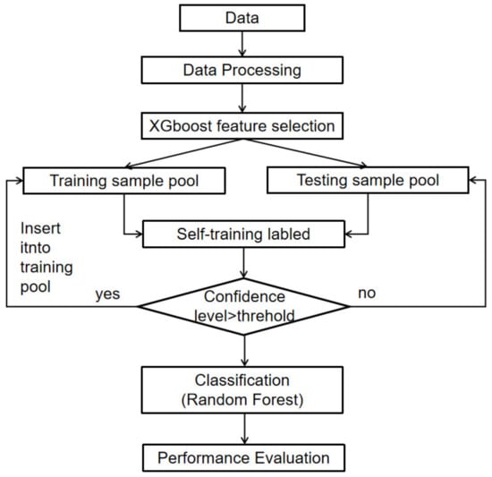
Figure 1.
The flowchart of the proposed semi-supervised FDD approach for AHU faults.
2.2. Feature Selection Based on XGboost
As a nonparametric model of supervised learning, the XGBoost algorithm is a kind of very effective machine learning algorithm, where the basic idea is to do a second-order Taylor expansion of the target function, using the function of the second derivative information to train a tree model, and the tree model complexity, as a regular item, is added to the optimization goal, making the model generalization ability higher learning [29,30,31]. The choice of the XGboost parameter depends on the training data used in the model, and its objective function is:
where is the true value of the ith target; is the predicted value of the ith target; describes the difference between and n is the number of samples; Ω(ƒk) is the tree model complexity of the kth sample characteristic parameter ƒk. K is the total amount of sample characteristic parameters.
Through optimization in the gradient direction, the model obtained before each iteration will be retained, and a new function will be added each time to improve the performance of the whole model, and the model residual of the weak learner will be continuously reduced to obtain a new tree model.
Therefore, in the t iteration step calculation, the training objective function O is transformed as follows:
where is the tree structure value of input variable in the tth iteration step calculation, and C is a constant.
At this point, when the target function is approximated by the second-order Taylor expansion, then:
where and are the first and second derivatives of the prediction error to the current model, respectively.
The constant term is removed and Equation (4) is expanded so that the objective function only depends on the first and second derivatives of each data point on the error function. At the same time, considering the decision tree model and defining the complexity of the tree, the objective function is further rewritten into the following form:
where is the output fraction of each leaf node; is the set for each leaf above sample collection; is the number of leaf nodes in the split tree; and are weighting factors used to control the specific gravity of the corresponding part.
As the model iterates, it optimizes itself based on residuals. At the same time, because the objective function of node-splitting is considered fully in the error term and regularization term, the model has high precision and good performance against over-fitting. Figure 2 shows how XGboost works.
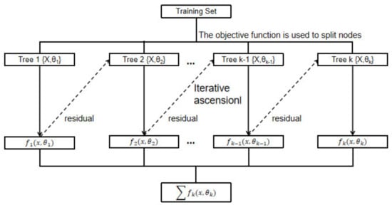
Figure 2.
How the XGboost algorithm works.
XGBoost effectively processes more distributed and irregular data, resulting in good overall model performance. The XGBoost algorithm optimizes CPU memory operations through parallel computing, making XGBoost a more versatile model for data, classification, and feature recognition. XGBoost utilizes the principles of enhanced ensemble learning algorithms to better predict performance. It increases the weight of misclassified training samples (the error rate is very high) and decreases the weight of correctly classified training samples. Previous misclassified training samples have a heavier weight, which can be processed several times to improve accuracy and reduce the error rate [30,31].
2.3. Random Forest Algorithm
Random forest (RF) has the advantages of processing large-scale data, preventing over-fitting and directly predicting new samples, and can provide good generalization performance for many fault diagnosis cases [30,31,32,33]. Random forest is a combinatorial learning algorithm containing multiple classifiers, including k independent classifiers , ..., , which can be expressed as:
where T is the input factor set, namely the characteristic data set, ( = 1,2... K) is the base classifier, and each classifier is a decision tree following the classification and regression tree (CART) method. The type that received the most votes was RF, which is the result of whether the corresponding AHU running state is faulty or not. The principle of RF is shown in Figure 3.
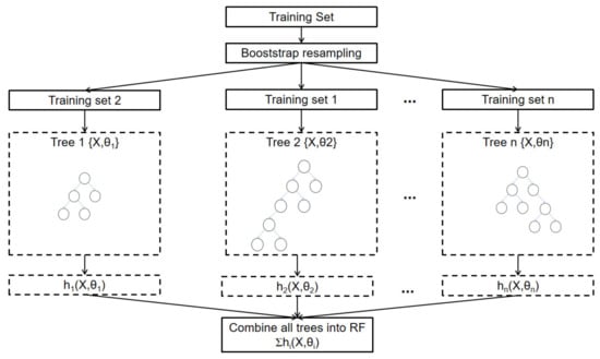
Figure 3.
Random forest operation principle.
When the air conditioning system fails, the collected characteristic information will change. The operating status of the air conditioning system can be judged by comparing the difference between the actual operating data and the preset baseline [34,35,36,37,38].
The main steps of RF fault diagnosis are briefly summarized as follows:
- Step 1: Extract features from the original data set to form a feature set. Feature subsets are formed by random drawing. The feature subset is the key factor in the growing process of each decision tree.
- Step 2: Select each bootstrap sample subset from the original fault sample set and replace it. The number of samples in the bootstrap sample subset is the same as in the original sample set. For each bootstrap sample set, approximately one-third of the samples from the original sample set, which make up the out-of-pocket (OOB) data set, are omitted.
- Step 3: Each decision tree is grown with a subset of bootstrap samples and a subset of features, following the CART approach.
- Step 4: The classification result of RF is provided by voting, and the fault diagnosis result is obtained based on it.
From the above flow chart, it can be seen that the construction of RF fault diagnosis model needs the data of the fault air conditioning system to train the model. The formation process mainly includes signal acquisition, feature selection and feature vector construction [39]. The random forest operation flow used in this research is shown in Figure 4.

Figure 4.
Random forest operation flow.
2.4. Self-Training Methods
Self-training, also known as self-study or self-labeling [40,41,42], is a simple semi-supervised learning method which has been widely used in many fields, such as image recognition and natural language processing. Self-training methods do not require any specific pre-assumptions, and self-training enables learning tasks to be trained on limited labeled training data, which shows impressive results in semi-supervised learning. The basic idea of self-training is to use the existing marked data to mark the unmarked data, so as to obtain more reliable training data. Specifically, the method first trains the model with labeled data, and then uses the model to predict unlabeled data. Finally, the unlabeled data with false labels are added to the training set to participate in further training, and the above process is repeated until the algorithm reaches the predetermined condition. The whole process can be summarized into the following steps:
- All labeled and unlabeled numbers are collected, and the labeled data (initial training set) are used to train the first supervised model, namely the basic classifier, which is used to predict the category of unlabeled data during training.
- The initial model is used to predict the categories of unlabeled data, observations that meet predefined criteria are selected (usually consisting of several unlabeled examples with high confidence predictions), and the initial training set is combined with its predicted labels to train the new classifier (selection step).
- The classifier is then retrained on a new set of token examples, and the process (the retraining step) is repeated until the stop condition is reached.
On this basis, the self-training model framework based on random forest proposed in this study is shown in Figure 5.
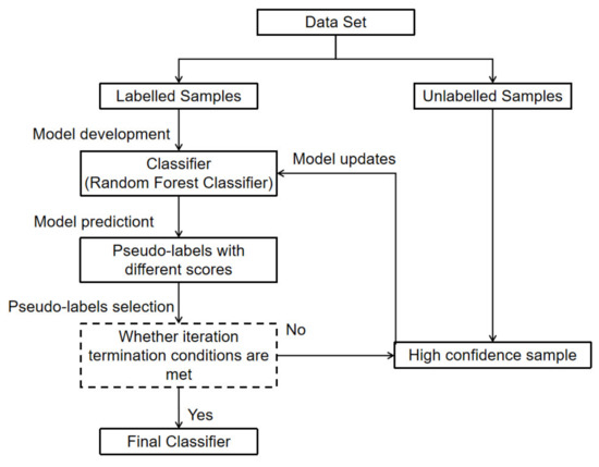
Figure 5.
A semi-supervised learning framework based on random forest.
3. Data Experiment
3.1. Data Description
In this study, the AHU operational data collected by the American Society of Heating, Refrigerating and Air-Conditioning Engineers (ASHRAE) research project RP-1312 were adopted for data experiments [43]. The raw data consisted of operation data, which were collected in three test periods: summer 2007, spring 2008, and winter 2008, each lasting two to three weeks. In the experiment, a number of operating faults were manually introduced to simulate the failure of the damper, fan and water coil, and detailed data records of the AHU operating status were collected at 1 min intervals. In this study, three main fault types were considered, each of which had three sub-types for data experiments. Considering the possible differences in data characteristics between different faults and the characteristics of random forest, the fault diagnosis task was set as three independent random forest classification problems. Table 1 summarizes the amount of data for different data labels. Considering the impact of data imbalance and randomness, different types of AHU failure data were mixed and randomly selected 2160 data and non-failure data were mixed to prepare for subsequent data processing.

Table 1.
A summary on data selected for analysis.
The experimental data were divided into training data and testing data, accounting for 75% and 25%, respectively. The training data were used to establish a semi-supervised random forest, and the testing data were used to evaluate the generalization performance. Secondly, 5%, 15%, 20%, 25% and 30% of the training data were extracted, respectively, and their original labels were retained while removing the labels of the remaining data. The labels were changed to 0 (normal operation state) or 1 (fault operation state) before data sampling. The different thresholds (i.e., 0.65, 0.75, 0.85 and 0.95) and the proportion of reserved marker data are shown in Table 2 to quantify their impact on semi-supervised fault detection and diagnosis. The maximum number of iterations of tag training was set to 100.
Table 2.
The experiment setups for fault diagnosis.
In this study, three main AHU fault types, each with three subtypes, were selected for the experiments. As shown in Table 1, there were 12,960 samples in the experimental data, including 10 unique labels, namely, where one was the normal operation state, and the rest were different types of wrong operations. Considering different faults and data characteristics, the importance of different variables may be different. Therefore, the statistical characteristics of variables under different fault types were determined after feature selection, as detailed in Section 3.2.
3.2. Feature Importance Selection
The basic idea of feature selection is to delete the functions that have little impact on the performance of the Machine Learning (ML) model, and only keep the functions that have the greatest impact on the ML model. Therefore, in the case of a given high-dimensional data set, dimension reduction through feature selection can reduce the amount of data, speed up the computation and improve the computational efficiency while ensuring the effect [41,42,43]. The characteristic space studied in this paper is 164-dimensional. There is one type of data in factor space, that is, the value. Numerical data are data with quantitative values, which are divided into numerical data directly related to the running state and numerical data that explain experimental attributes (e.g., the date, or time nodes). Another important issue is dealing with lost data. Missing values often exist in data sets for a variety of reasons, so it is important to propose solutions that can fill in such null values if there are data missing before further modeling. None of the three fault types exist in the existing experimental data.
The fault feature is extracted from the original data, which mainly reflects the relationship between a feature and the fault label, that is, the importance of feature. It is generally believed that the more important a feature is, the more influence it has on fault diagnosis. By applying the XGboost method described in Section 2 to the data set described in Section 3.1, the immediate result will be a ranking of the importance of features. The ranking of feature importance under different fault types is shown in Figure 6, Figure 7 and Figure 8. For the fault type EA Stuck, the data dimension reduced from 164 to 16. For the fault type OA Stuck, the data dimension decreased from 164 to 13. For the fault type Cooling Coil Valve Stuck, the data dimension decreased from 164 to 8. It can be seen from the above results that the same feature data have different influences on different fault categories.
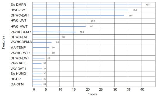
Figure 6.
The feature importance of EA Damper stuck.
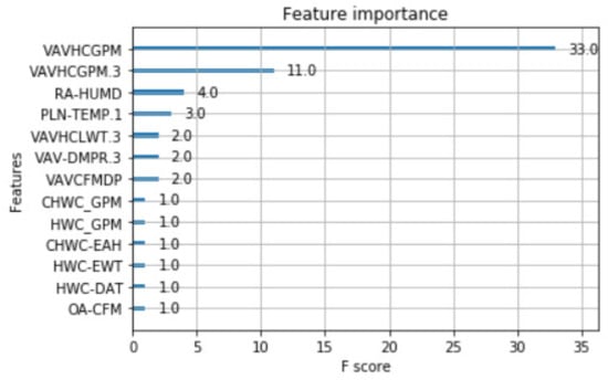
Figure 7.
The feature importance of OA Damper stuck.
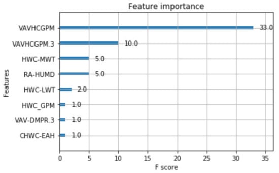
Figure 8.
The feature importance of Cooling Coil Valve Stuck.
Based on feature selection results, 26 variables were selected as model inputs variables considering their importance in fault detection. The statistical characteristics of these variables are summarized in Table 3.
Table 3.
The statistical characteristics of model input variables.
3.3. Random Forest Model Training
Random Forest (RF) is an ensemble learning algorithm with multiple classifiers. The RF algorithm model is built by adding a certain number of decision trees, using a resampling data set from the original training data. The decision tree for each component is grown by the classification and Regression Tree (CART) algorithm. In principle, two random attributes are introduced when building decision trees. The basic principle is that there are a lot of training data inputs based on decision trees, among which the training data in each tree are different, the features needed for each tree construction are randomly selected from the overall features, and finally, votes are used to select the most likely classification results.
In order to verify the influence of feature selection on the classification results of the random forest model, the original data before and after dimension reduction were respectively input as data on the basis of ensuring the consistency of model parameters, and the performance differences of different training data under the random forest classifier were compared.
3.4. Add Pseudo-Labels by Self-Training
On the basis of feature selection, the data were segmented to support the needs of label training. First, the data were divided into test data and training data by 25% and 75%, respectively. The training data were used to train the model, and the test data were used to evaluate the performance of the model. As the experimental data used in this study were all labeled data, we simulated the situation of unlabeled data by deleting some labels with labeled data. The labeled data were retained in 5%, 15%, 20%, 25% and 30% of the data set, respectively, and the labels of the remaining data were masked. The data set was artificially divided into labeled data and unlabeled data.
The processed data were used as input data for model training and model performance evaluation, respectively, and the trained classifier was used to predict the labels of all unlabeled data. Among these predicted labels, those whose accuracy reached the set threshold were considered as “false labels” and were re-assigned with labels. The “false label” data were connected with the original labeled training data, and the classifier was retrained on the combined “false label” and the original labeled training data. Considering the influence of threshold-setting on label prediction and final classification results, the thresholds were set as 0.65, 0.75, 0.85, and 0.95, respectively, and the classification performance under different thresholds was evaluated.
4. Results and Discussion
4.1. Feature Importance and Feature Correlation Analysis
In order to further verify the impact of feature dimension reduction on the classification task, we input the original data and the dimension reduction data as data, respectively, and compared the classification results of the random forest model before and after dimension reduction. There are many indicators which can be used to evaluate the performance of classification models, and the following four indicators are mainly considered in this study:
- Precision: Precision refers to the correct prediction percentage of each class, the number of evaluated samples in each class, and the proportion of positive samples in positive examples judged by the classifier. Its expression can be expressed as:
- Recall: Recall is the percentage of predicted positive examples in the total positive examples, and it is the percentage of correctly predicted entities in a class. It is the correlation between the number of correctly predicted instances and the sum of correctly missed predictions of the class, and its expression is expressed as follows.
- F1-score: The F1-score is used in statistics to measure the accuracy of binary classification models. It takes into account both the accuracy and recall of the classification model. The F1-score can be regarded as a harmonic average of model accuracy and recall, with a maximum value of 1 and a minimum value of 0. Its expression can be expressed as:
- Accuracy Score: Accuracy refers to the percentage of the overall model that is correctly predicted among the total number of samples used to test the model, and represents the proportion of the classifier that is correctly judged by the whole sample. Its expression can be expressed as:
Among them:
- Accuracy True Positive (TP): The predicted answer is correct, judged to be a positive sample, and it is actually a positive sample.
- True Negative (TN): The predicted answer is correct, judged to be a negative sample, and it is actually a negative sample.
- False Positive (FP): The predicted answer indicates that another class is incorrectly predicted as this class.
- False Negative (FN): The label of the category is predicted to be of another category.
The result of accuracy is shown in Figure 9. Accuracy is the ratio between the number of correctly classified positive samples and the total number of correctly classified positive samples (correct or incorrect). Accuracy measures how well a model classifies a sample as positive.
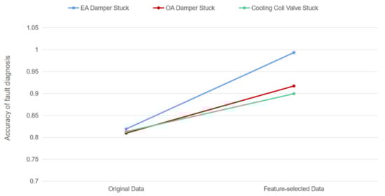
Figure 9.
The effect of feature selection on random forest classification.
The confusion matrix is a basic tool for model performance [44]. It summarizes the classification results, mainly the number of correct predictions and the number of incorrect predictions for each class. From the confusion matrix, accuracy, precision and recall can be calculated. It is important to note that accuracy measures the performance of the entire model, while precision and recall provide insight into specific classes. The original sample data of different fault types and the sample data after feature selection were taken as input, and the confusion matrix is shown in Figure 10 and Figure 11.
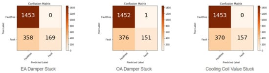
Figure 10.
Confusion Matrix based on original data set.
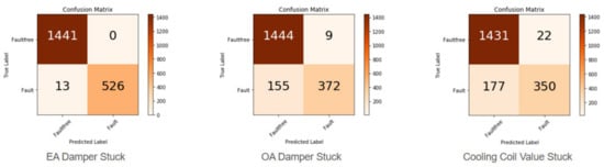
Figure 11.
Confusion Matrix based on feature-selected data set.
The diagonal cells in Figure 10 and Figure 11 are the correct predicted counts for each class. The remaining cells are the counts of instances with all incorrect predictions.
According to the confusion matrix results, Table 4 and Table 5 summarize the performance index results before and after the feature dimension reduction, which is convenient for us to analyze and quickly detect the model with excellent performance.
Table 4.
Classification models’ summary results before feature-selection.
Table 5.
Classification models’ summary results after feature-selection.
From the above results, it can be clearly seen that the evaluation indexes of the RF classification model after dimension reduction by the XGboost algorithm were improved, and better output was obtained in general. Although the improvement effect of different fault types is different, the classification accuracy was improved by about 10%, which has a significant impact on the fault diagnosis and operation performance evaluation of the air conditioning system.
In order to further analyze the effectiveness of dimensionality reduction, correlation analysis was carried out on the data features after dimensionality reduction. The heatmap, also known as correlation coefficient map, can judge the correlation between variables according to the size of the correlation coefficient corresponding to different square colors in the thermal map. In this study, the Pearson product-moment correlation coefficient (PPMCC) was mainly used to measure the correlation degree (linear correlation) between two variables X and Y, and its value was between −1 and 1. The specific formula is as follows:
However, it should be noted that the correlation coefficient can only measure the linear correlation between variables. In other words, the higher the correlation coefficient, the stronger the degree of linear correlation between variables; the lower the correlation coefficient, the weaker the degree of linear correlation between variables, but it does not mean that there is no other correlation between variables. Figure 12, Figure 13 and Figure 14 show the feature correlation of different fault types. Considering the improvement of classification performance, feature dimension reduction is still necessary and meaningful.
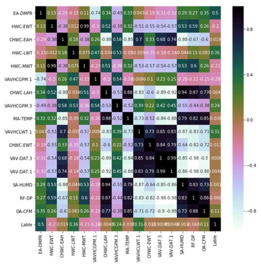
Figure 12.
Feature correlation based on feature-selected data set of EA Damper Stuck.
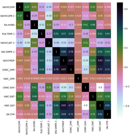
Figure 13.
Feature correlation based on feature-selected data set of OA Damper Stuck.
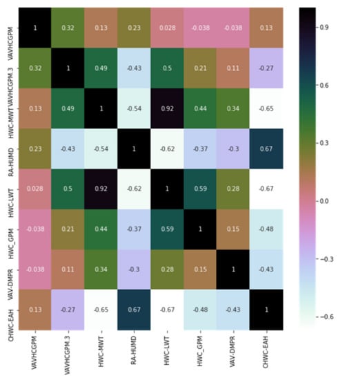
Figure 14.
Feature correlation based on feature-selected data set of Cooling Coil Valve Stuck.
4.2. Self-Training Parameters and Performance Evaluation
Figure 15 shows the fault diagnosis performance of semi-supervised learning under different parameter conditions. In general, there is an increasing trend between the number of labeled data and the fault diagnosis accuracy. This is expected because the larger the amount of labeled data, the more reliable the model generalization performance. In the early stages, as the number of labeled data per class increases, a significant improvement in fault diagnosis accuracy is generally observed, but there are also fluctuations. Through reviewing relevant literature, the following two possible reasons are considered for the occurrence of this situation:
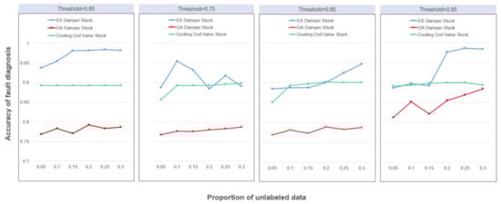
Figure 15.
The accuracy of fault diagnosis using semi-supervised RF.
- Limitations of the self-training label approach. The self-training method uses trained classifiers to predict the class labels of all unlabeled data instances. The predicted labels that meet the threshold requirements can be used as “pseudo-labels” at the same time. The “pseudo-labeled” data are combined with the original labeled training data and the classifier is retrained on this basis. Considering the proportion of the masked label data, the accuracy of “false label” prediction may have a great impact on the classification results.
- The label masking process may change the distribution of the original data. Since the original experimental data are all labeled data, the unlabeled data are simulated by masking a certain proportion of the original data labels. However, the label-masking process is random, and this randomness may change the data distribution. When the proportion of the masked label data changes, the data distribution may also change. The accuracy of fault diagnosis decreases as the proportion of data that retains the original marker increases.
At the same time, with an increase of the preset threshold, it can be observed that the accuracy of fault diagnosis is generally significantly improved. The higher the preset threshold, the higher the reliability of pseudo-label prediction. At the same time, when the number of each type of labeled data reaches a certain critical value, the accuracy of fault diagnosis tends to be stable. In this case, it is difficult to further improve the generalization performance by increasing the proportion of labeled data in the data set.
However, the effect of the pseudo-labeled data selection threshold on semi-supervised learning performance is contradictory in nature. On the one hand, a larger threshold can improve the reliability of the selected pseudo-labels, which is conducive to the stability of the model training process and the reliability of the classification results. On the other hand, a larger threshold will reduce the amount of pseudo-labeled data in semi-supervised learning, thus reducing the utilization efficiency of non-labeled data in semi-supervised learning. For example, when the faulty OA DAMPER STUCK’s faulty data label masking rate is 0.1, 4195 new labels are added after one iteration when the threshold is 0.65, and only three new labels are added after one iteration when the threshold is raised to 0.95 under the same conditions.
5. Conclusions
The development and application of building information technology provide a large amount of monitoring data for the automation and intelligence of building operation management [45]. It is very promising and practical to apply powerful machine learning techniques to develop reliable and accurate data-driven models to establish system fault detection and diagnosis. However, these building operation data are often unlabeled, which limits the application of traditional machine learning on operation data. To solve this problem, this paper proposed a semi-supervised learning method for fault detection and the diagnosis of air conditioning systems. In order to make effective use of building operation data, a new method based on semi-supervised neural network was proposed. Through a real data experiment, the role and effect of the method in typical fault identification of the air-conditioning system are verified. The research method can be used to develop advanced data-driven tools to extract key features to analyze and utilize a large number of building operation data. The results show that the proposed semi-supervised learning method can make full use of unlabeled data for fault detection and diagnosis of building systems. First of all, in the case of limited labeled data, the random forest classification method can obtain good fault diagnosis performance, and its original accuracy reached about 0.81 on average before subsequent processing. Second, the XGboost method can effectively reduce the dimensions of the data set, and the three kinds of different fault types effectively reduced the feature dimension, reduced the feature dimension from three digits to double digits, the feature dimension reduction after different types of fault diagnosis accuracy increased to 0.91 or so, and reduced the redundant features of the influence of the fault diagnosis, which was helpful to improve the operation efficiency and effectiveness. Meanwhile, parameter settings have different effects on diagnosis results of different fault types, but overall, with the increase of the proportion of labeled data and threshold, the fault diagnosis rate also increased. Only the EA Damper Stuck had a large fluctuation. The following two reasons are mainly considered:
- The compatibility of the fault feature with the proposed method was lower than that of the other two types;
- Compared with the other two fault categories, the adaptability of the data collected from the experiment and the proposed method was lower.
However, this study also has some shortcomings. For example, in feature dimension reduction, there may have been some correlation between the extracted key features, and the actual impact of this correlation on the classification results has not been verified. The exact physical meaning of the features was not illustrated clearly. The data used in the paper and the applicability of the proposed method have not been verified in advance. Due to the limitation of objective conditions, this study used the existing historical experimental data to simulate the actual collection of unlabeled data by randomly masking existing labels. However, the randomness of label masking may modify the actual distribution of experimental data, thus affecting the classification performance. Therefore, in future research, based on considering the applicability of the used data and the designed methods, feature engineering can be used to comprehensively preprocess the data features, and dimensionality reduction can be carried out on the basis of fully considering the existing feature attributes and correlations. At the same time, relevant experiments can be set up in practice to collect real-time operation data of the air conditioning system, and further demonstrate the role and significance of the semi-supervised learning method in practical fault diagnosis work.
Author Contributions
Conceptualization, G.M. and H.D.; methodology, G.M. and H.D.; software, H.D.; validation, H.D.; formal analysis, H.D.; investigation, H.D.; resources, G.M.; data curation, H.D.; validation, H.D.; writing—original draft preparation, H.D.; writing—review and editing, H.D.; supervision, G.M.; project administration, G.M.; funding acquisition, G.M. All authors have read and agreed to the published version of the manuscript.
Funding
This research received no external funding.
Data Availability Statement
The data was bought on https://www.techstreet.com/ashrae/standards/rp-1312-tools-for-evaluating-fault-detection-and-diagnostic-methods-for-air-handling-units?product_id=1833299 (accessed on 10 September 2022), which was open to use.
Conflicts of Interest
The authors declare no conflict of interest.
References
- Global Alliance for Buildings and Construction. 2018 Global Status Report: Towards a Zero Emission, Efficient and Resilient Buildings and Construction Sector; United Nation Environment: Nairobi, Kenya, 2018; ISBN 978-92-807-3729-5. [Google Scholar]
- Nyboer, J. Energy Use and Related Data: Canadian Electricity Generation Industry 1990 to 2012; CIEEDAC: Burnaby, Canada, 2012. [Google Scholar]
- Bruton, K.; Raftery, P.; O’Donovan, P.; Aughney, N.; Keane, M.M.; O’Sullivan, D.T.J. Development and alpha testing of a cloud based automated fault detection and diagnosis tool for Air Handling Units. Autom. Constr. 2014, 39, 70–83. [Google Scholar] [CrossRef]
- 2011 Building Energy Handbook from DOE. 14 February 2013. Available online: http://web.archive.org/web/20130214212606/http://buildingsdtabook.eren.doe.gov/docs/DataBooks/2011_BEDB.pdf (accessed on 10 April 2021).
- Gholamzadehmir, M.; Del Pero, C.; Buffa, S.; Fedrizzi, R. Adaptive-predictive control strategy for HVAC systems in smart buildings—A review. Sustain. Cities Soc. 2020, 63, 102480. [Google Scholar] [CrossRef]
- Lin, G.; Kramer, H.; Granderson, J. Building fault detection and diagnostics: Achieved savings, and methods to evaluate algorithm performance. Build. Environ. 2020, 168, 106505. [Google Scholar] [CrossRef]
- Yu, Y.; Woradechjumroen, D.; Yu, D. A review of fault detection and diagnosis methodologies on air-handling units. Energy Build. 2014, 82, 550–562. [Google Scholar] [CrossRef]
- Zhao, Y.; Li, T.; Zhang, X.; Zhang, C. Artificial intelligence-based fault detection and diagnosis methods for building energy systems: Advantages, challenges and the future. Renew. Sustain. Energy Rev. 2019, 109, 85–101. [Google Scholar] [CrossRef]
- Fan, C.; Liu, X.; Xue, P.; Wang, J. Statistical characterization of semi-supervised neural networks for fault detection and diagnosis of air handling units. Energy Build. 2021, 234, 110733. [Google Scholar] [CrossRef]
- Mills, E.; Bourassa, N.; Piette, M.A.; Friedman, H.; Haasl, T.; Powell, T.; Claridge, D. The cost-effectiveness of commissioning new and existing commercial buildings: Lessons from 224 buildings. In Proceedings of the National Conference on Building Commissioning, New York, NY, USA, 4–6 May 2005. [Google Scholar]
- Sha, H.; Xu, P.; Hu, C.; Li, Z.; Chen, Y.; Chen, Z. A simplified HVAC energy prediction method based on degree-day. Sustain. Cities Soc. 2019, 51, 101698. [Google Scholar] [CrossRef]
- Li, D.; Zhou, Y.; Hu, G.; Spanos, C.J. Optimal sensor configuration and feature selection for AHU fault detection and diagnosis. IEEE Trans. Ind. Inform. 2016, 13, 1369–1380. [Google Scholar] [CrossRef]
- Chen, J.; Zhang, L.; Li, Y.; Shi, Y.; Gao, X.; Hu, Y. A review of computing-based automated fault detection and diagnosis of heating, ventilation and air conditioning systems. Renew. Sustain. Energy Rev. 2022, 161, 112395. [Google Scholar] [CrossRef]
- Sterling, R.; Provan, G.; Febres, J.; O’Sullivan, D.; Struss, P.; Keane, M.M. Model-based fault detection and diagnosis of air handling units: A comparison of methodologies. Energy Procedia 2014, 62, 686–693. [Google Scholar] [CrossRef]
- Yan, X.; Jia, M. A novel optimized SVM classification algorithm with multi-domain feature and its application to fault diagnosis of rolling bearing. Neurocomputing 2018, 313, 47–64. [Google Scholar] [CrossRef]
- Wang, H.; Feng, D.; Liu, K. Fault detection and diagnosis for multiple faults of VAV terminals using self-adaptive model and layered random forest. Build. Environ. 2021, 193, 107667. [Google Scholar] [CrossRef]
- Xiao, F.; Zhao, Y.; Wen, J.; Wang, S. Bayesian network based FDD strategy for variable air volume terminals. Autom. Constr. 2014, 41, 106–118. [Google Scholar] [CrossRef]
- Gao, Z.; Cecati, C.; Ding, S.X. A survey of fault diagnosis and fault-tolerant techniques—Part I: Fault diagnosis with model-based and signal-based approaches. IEEE Trans. Ind. Electron. 2015, 62, 3757–3767. [Google Scholar] [CrossRef]
- Fan, C.; Li, X.; Zhao, Y.; Wang, J. Quantitative assessments on advanced data synthesis strategies for enhancing imbalanced AHU fault diagnosis performance. Energy Build. 2021, 252, 111423. [Google Scholar] [CrossRef]
- Zhu, X.; Goldberg, A.B. Introduction to semi-supervised learning. Synth. Lect. Artif. Intell. Mach. Learn. 2009, 3, 1–130. [Google Scholar]
- Guo, Y.; Chen, H. Fault diagnosis of VRF air-conditioning system based on improved Gaussian mixture model with PCA approach. Int. J. Refrig. 2020, 118, 1–11. [Google Scholar] [CrossRef]
- Fan, Y.; Cui, X.; Han, H.; Lu, H. Chiller fault diagnosis with field sensors using the technology of imbalanced data. Appl. Therm. Eng. 2019, 159, 113933. [Google Scholar] [CrossRef]
- Zhou, Q.; Wang, S.; Xiao, F. A novel strategy for the fault detection and diagnosis of centrifugal chiller systems. HVAC&R Res. 2009, 15, 57–75. [Google Scholar]
- Van Every, P.M.; Rodriguez, M.; Jones, C.B.; Mammoli, A.A.; Martínez-Ramón, M. Advanced detection of HVAC faults using unsupervised SVM novelty detection and Gaussian process models. Energy Build. 2017, 149, 216–224. [Google Scholar] [CrossRef]
- Zhu, X.; Du, Z.; Jin, X.; Chen, Z. Fault diagnosis based operation risk evaluation for air conditioning systems in data centers. Build. Environ. 2019, 163, 106319. [Google Scholar] [CrossRef]
- Li, G.; Chen, H.; Hu, Y.; Wang, J.; Guo, Y.; Liu, J.; Li, H.; Huang, R.; Lv, H.; Li, J. An improved decision tree-based fault diagnosis method for practical variable refrigerant flow system using virtual sensor-based fault indicators. Appl. Therm. Eng. 2018, 129, 1292–1303. [Google Scholar] [CrossRef]
- Subramanya, A.; Talukdar, P.P. Graph-based semi-supervised learning. Synth. Lect. Artif. Intell. Mach. Learn. 2014, 8, 1–125. [Google Scholar]
- Yu, K.; Lin, T.R.; Ma, H.; Li, X.; Li, X. A multi-stage semi-supervised learning approach for intelligent fault diagnosis of rolling bearing using data augmentation and metric learning. Mech. Syst. Signal Process. 2021, 146, 107043. [Google Scholar] [CrossRef]
- Qiao, Z.; Lei, Y.; Li, N. Applications of stochastic resonance to machinery fault detection: A review and tutorial. Mech. Syst. Signal Process. 2019, 122, 502–536. [Google Scholar] [CrossRef]
- Hu, Q.; Si, X.S.; Zhang, Q.H.; Qin, A.S. A rotating machinery fault diagnosis method based on multi-scale dimensionless in-dicators and random forests. Mech. Syst. Signal Process. 2020, 139, 106609. [Google Scholar] [CrossRef]
- Sanchez, R.V.; Lucero, P.; Vásquez, R.E.; Cerrada, M.; Macancela, J.C.; Cabrera, D. Feature ranking for multi-fault diagnosis of rotating machinery by using random forest and KNN. J. Intell. Fuzzy Syst. 2018, 34, 3463–3473. [Google Scholar] [CrossRef]
- Li, Z.; Jin, H.; Dong, S.; Qian, B.; Yang, B.; Chen, X. Semi-supervised ensemble support vector regression based soft sensor for key quality variable estimation of nonlinear industrial processes with limited labeled data. Chem. Eng. Res. Des. 2022, 179, 510–526. [Google Scholar] [CrossRef]
- Mehyadin, A.E.; Abdulazeez, A.M. Classification based on semi-supervised learning: A review. Iraqi J. Comput. Inform. 2021, 47, 1–11. [Google Scholar]
- Patel, R.K.; Giri, V.K. Feature selection and classification of mechanical fault of an induction motor using random forest classifier. Perspect. Sci. 2016, 8, 334–337. [Google Scholar] [CrossRef]
- He, H.; Zhang, W.; Zhang, S. A novel ensemble method for credit scoring: Adaption of different imbalance ratios. Expert Syst. Appl. 2018, 98, 105–117. [Google Scholar] [CrossRef]
- Li, M.; Dai, L.; Hu, Y. Machine learning for harnessing thermal energy: From materials discovery to system optimization. ACS Energy Lett. 2022, 7, 3204–3226. [Google Scholar] [CrossRef]
- Paul, A.; Mukherjee, D.P.; Das, P.; Gangopadhyay, A.; Chintha, A.R.; Kundu, S. Improved random forest for classification. IEEE Trans. Image Process. 2018, 27, 4012–4024. [Google Scholar] [CrossRef] [PubMed]
- Liu, Y.; Wang, Y.; Zhang, J. New machine learning algorithm: Random forest. In Proceedings of the ICICA 2012: Information Computing and Applications, Proceedings of the International Conference on Information Computing and Applications, Chengde, China, 14–16 September 2012; Springer: Berlin/Heidelberg, Germany, 2012; pp. 246–252. [Google Scholar]
- Chen, S.; Yang, R.; Zhong, M. Graph-based semi-supervised random forest for rotating machinery gearbox fault diagnosis. Control. Eng. Pract. 2021, 117, 104952. [Google Scholar] [CrossRef]
- Chen, C.; Zhang, Y.; Gao, Y. Learning how to self-learn: Enhancing self-training using neural reinforcement learning. In Proceedings of the 2018 International Conference on Asian Language Processing (IALP), Bandung, Indonesia, 15–17 November 2018; pp. 25–30. [Google Scholar]
- Nartey, O.T.; Yang, G.; Wu, J.; Asare, S.K. Semi-supervised learning for fine-grained classification with self-training. IEEE Access 2019, 8, 2109–2121. [Google Scholar] [CrossRef]
- Wen, J.; Li, S. Tools for Evaluating Fault Detection and Diagnostic Methods for Air-Handling Units; ASHRAE RP-1312 Final Report; American Society of Heating, Refrigerating and Air-Conditioning Engineers: Atlanta, GA, USA, 2011. [Google Scholar]
- Piscitelli, M.S.; Mazzarelli, D.M.; Capozzoli, A. Enhancing operational performance of AHUs through an advanced fault detection and diagnosis process based on temporal association and decision rules. Energy Build. 2020, 226, 110369. [Google Scholar] [CrossRef]
- Fan, C.; Xiao, F.; Li, Z.; Wang, J. Unsupervised data analytics in mining big building operational data for energy efficiency enhancement: A review. Energy Build. 2018, 159, 296–308. [Google Scholar] [CrossRef]
- Yin, Z.; Hou, J. Recent advances on SVM based fault diagnosis and process monitoring in complicated industrial processes. Neurocomputing 2016, 174, 643–650. [Google Scholar] [CrossRef]


Disclaimer/Publisher’s Note: The statements, opinions and data contained in all publications are solely those of the individual author(s) and contributor(s) and not of MDPI and/or the editor(s). MDPI and/or the editor(s) disclaim responsibility for any injury to people or property resulting from any ideas, methods, instructions or products referred to in the content. |
© 2022 by the authors. Licensee MDPI, Basel, Switzerland. This article is an open access article distributed under the terms and conditions of the Creative Commons Attribution (CC BY) license (https://creativecommons.org/licenses/by/4.0/).