
Optimum Cost Prediction of Reinforced Concrete Cantilever Retaining Walls

Civil Engineering Department, Atılım University, 06830 Ankara, Turkey
Buildings 2023, 13(10), 2409; https://doi.org/10.3390/buildings13102409
Submission received: 10 August 2023
/
Revised: 13 September 2023
/
Accepted: 20 September 2023
/
Published: 22 September 2023
Abstract
:Reinforced concrete cantilever retaining walls (RCCRWs) are widely used in civil engineering projects as a common type of retaining structure. The design of these structures focuses on ensuring safety against various failure scenarios and compliance with standard building code requirements. This research aims to enhance the design process of RCCRWs by developing a specific code and optimizing it through a metaheuristic-based algorithm. In this study, the cost prediction of RCCRWs is also investigated through a parametric study involving key variables such as wall height, seismic zone, backfill material properties, and backfill inclination angle. To achieve this, non-linear regression analysis is employed to establish an empirical correlation, enabling cost estimation for optimized RCCRWs. The resulting prediction equation is simple to use, requiring only limited inputs. Therefore, it can be applied during the initial stages of a project, making a valuable contribution in determining approximate costs for RCCRW projects.
1. Introduction
Reinforced concrete cantilever retaining walls (RCCRWs) are commonly employed in various civil engineering projects to stabilize natural slopes or artificial cuts in highways, bridges and other constructions. In the design of RCCRWs, the selection of the appropriate wall dimensions is crucial since it dramatically affects both the stability and cost. Optimization techniques have found extensive applications in different areas of civil engineering, such as project time–cost estimation [1], risk–cost maintenance strategy [2], optimization of structures [3,4,5,6], damage detection [7] and water distribution network optimization [8]. Numerous studies have been conducted to optimize the size of retaining walls, with the aim of achieving cost-effective designs [9]. Most of the methods focus on achieving cost-effective and lightweight RCCRWs through the utilization of various optimization tools. These optimization techniques often involve metaheuristic algorithms [10], such as the particle swarm optimization [11,12], modified particle swarm optimization [13], colony optimization [14], artificial bee colony algorithm [15], genetic algorithm [16], harmony search algorithm [17], evolution strategy [18,19] and simulated annealing [20,21]. Previous studies using these approaches consistently identify the wall height as the most critical parameter for optimizing RCCRWs. On the other hand, some studies show that the soil properties of the backfill also have a significant effect on the overall cost [15,19]. In a closely related study conducted by Yepes et al. [21], the cost prediction of RCCRWs was examined. The authors highlighted that the two most influential parameters impacting the cost of optimal walls are the sliding behavior and the fill type. Counterintuitively, the bearing capacity of the soil was found to have minimal impact on the costs of RCCRWs. Instead, the cost of optimized walls showed a parabolic correlation with the wall height.
Although there have been significant advancements in engineering design proce-dures, optimizing engineering structures is still a difficult task that requires a multidisci-plinary approach. Using different parameters to produce predictive models for optimum cost prediction of reinforced concrete cantilever walls been extensively studied in the re-cent literature [22]. There are few studies focused on predicting the costs of retaining walls using predictive equations, despite the fact that many researchers have investigated the optimization of retaining walls using different methodologies for specific design input parameters. This study aims to explore the impact of various parameters on the cost of RCCRWs. These parameters include the wall height, backfill material properties, backfill slope, design earthquake spectral response acceleration parameter at short period, and the equivalent static earthquake reduction coefficient. The goal is to establish an empirical correlation between these parameters and the cost of RCCRWs. To facilitate the optimization process, a MATLAB code is developed, according to the new Turkish Building Earthquake Specifications [23] and Turkish Standard Requirements for Design and Construction of Reinforced Concrete Structures [24] specific to RCCRWs. The optimization is performed using the “exponential big bang-big crunch algorithm”, a metaheuristic optimization method originally introduced by Hasançebi and Kazemzadeh [25], to attain a cost-effective design. The investigation involves 1080 different cases generated by using different values of the mentioned parameters to determine the minimum cost for RCCRWs. The total cost comprises the expenses of concrete, reinforcement, and backfill materials. Concurrently, non-linear regression analysis is applied to establish the relationship between the cost and the corresponding parameters. Finally, a parametric study comprising 180 cases is conducted to compare the actual costs with the predicted costs obtained from the established correlation. This comparison will validate the accuracy and effectiveness of the proposed prediction equation in estimating the costs of RCCRWs under different scenarios.
The remainder of this paper is organized as follows. In Section 2, the details of the design of the cantilever retaining walls are presented. Section 3 covers optimum design modelling. Regression analysis for cost prediction has been elaborated in Section 4. Finally, the concluding remarks have been provided in Section 5.
2. Design of Cantilever Retaining Walls
In the first part of the design, the preliminary dimensions of the RCCRW can be defined by using the wall height (H) and base width (B), according to Bowles [26], TS 7994 [27], and ACI 318 [28] as shown in Figure 1, and Table 1. Alternatively, the base width (B) can be determined as a function of the height. Using these sketches as a guide, the dimensions are selected, and the most cost-effective design is achieved through the conventional trial-and-error approach. This involves considering both internal and external stability conditions. For the cantilever wall to be safe and effective, it must not slide or overturn, and it should be safe in terms of bearing capacity to avoid failure. Once these external stability requirements are satisfied, the structural design must ensure that the cantilever wall is able to satisfy internal stability requirements [29,30].
In order to assess the external stability of the cantilever walls, several checks are conducted, including those for overturning, sliding and bearing capacity. For static conditions, the external stability analysis involves using the conventional factor of safety. On the other hand, for seismic conditions, the analyses are based on ultimate limit states. The dimensions and the loads acting on the RCCRW with a sloping backfill are depicted in Figure 2. In this figure, all the forces related to the static condition are shown. Here, W1, W2 and W3 are the weights of sections 1, 2 and 3 of the reinforced concrete retaining wall, W4 and W5 are the weights of the backfill acting on the heel of the wall, and W6 is the weight of the backfill acting on the toe of the wall. In addition, Pa is the force resulting from the active earth pressure due to the backfill, and Ppk and Pp are the forces resulting from the passive earth pressures in front of the toe section of the wall and on the base shear key, respectively. Pa and Pp are calculated by using Equations (1) and (2), and the force Ppk is generally neglected due to safety considerations. On the other hand, qmin and qmax are the minimum and maximum bearing stresses acting on the base of the wall.
In the seismic analyses, the total force acting on the wall (Pt) due to the backfill is calculated by using Equation (3). The additional seismic force (ΔPae) to active pressure, which is the difference between the total force and active force, is calculated by Equation (4). These analyses allow for a comprehensive evaluation of the external stability of cantilever walls under seismic conditions.
Here, γd, γ and c2 are the moist unit weight of the backfill soil, base soil and cohesion of the base soil, respectively. In addition, H is the height of the retaining wall, D′ is the height of the base shear key, β is the inclination of the backfill slope in degrees, and d is the heel part of the base of the RCCRW under the backfill (as shown in Figure 2). The coefficient of active earth pressure for the backfill (Ka, Equation (5)) must be calculated if its inclination is less than or equal to the difference in degrees between the friction angle of the backfill (Φ′d) and the pseudo static earthquake coefficient (θ, Equation (8)). Otherwise, it must be determined by using Equation (6) (for the static conditions, θ = 0). In Equation (7), Kp is the passive earth pressure coefficient used to calculate the passive forces acting on the cantilever wall, and Ψ and δd are the inclination of the back of the stem with respect to the horizontal axes and the angle of friction between the cantilever wall and the backfill soil, respectively. On the other hand, SDS in Equation (9) is the design earthquake spectral response acceleration parameter at a short period, and kh and kv in Equations (9) and (10) are the horizontal and vertical equivalent static earthquake coefficients, respectively. In addition, r is the equivalent static earthquake reduction coefficient. It can be taken as 1.5 or 2.0 for the walls having a maximum displacement of 80SDS (mm) and 120SDS (mm), respectively.
In seismic analyses, the design value of the resistance (Rt) is calculated by Equation (11) using the characteristic resistance (Rk) and the partial resistance factor (γR). The partial resistance factor values for bearing capacity (γRv), is suggested as 1.4, whereas it is recommended as 1.1 and 1.4 for sliding resistance (γRh) and passive earth resistance, (γRp) respectively [23].
The retaining wall is checked against overturning for static considerations first. Overturning occurs due to the unbalanced moments, and the factor of safety against overturning is calculated by using the ratio of summation of the resisting moments (MR) to the summation of the driving moments (MO) with respect to the toe of the cantilever wall, as shown in Equation (12).
In the assessment, the moments caused by the weight of the cantilever wall, backfill material and the vertical component of the earth pressure establish the resisting moments. On the other hand, the moment due to the backfill earth pressure is taken as the driving moment. In the calculations, the moments with respect to the backfill on the toe slab and the moments due to the passive resistance in front of the wall are neglected to be on the safe side. The minimum factor of safety against overturning is taken as 2.5.
For the seismic condition, the following equations are used:
Here, Wi is the weight of the associated section, and xi and yi are the corresponding moment arms with respect to the toe. Pav and Pah are the vertical and horizontal components of the active earth pressure, respectively. Furthermore, ΔPaev is the vertical component of the additional seismic force acting at an H′/2 distance from the bottom of the wall [21]. The ratio of the resisting moments (Rdev) to the driving moments (Edev) with respect to the toe of the wall must be equal or greater than the partial resistance factor (γRdev = 1.3) [21].
The evaluation of the sliding criterion represents a significant aspect of the external stability assessment. By analyzing the forces acting on the cantilever wall (Figure 2), both the resisting and sliding forces are determined. In addition, the passive resistance (with a factor of safety 2) due to the base shear key that is under the base slab is taken into consideration. The factor of safety against sliding (FSsliding in Equation (16)) is defined as the ratio of the horizontal resisting forces (FR in Equation (17)) to the horizontal driving forces (FD in Equation (18)). To satisfy the criterion FSsliding ≥ 1.5, a thorough assessment of the wall’s external stability is achieved through a comprehensive analysis of the resisting and sliding forces and the incorporation of passive resistance from the base shear key.
Here, ΣV is the total vertical force acting on the base, B is the length of the base, k1 and k2 are the reduction coefficients for the internal friction angle and the cohesion between the foundation soil and the cantilever wall, respectively, and Φ2 and c2 are the shear strength parameters of the foundation soil.
The safety check against sliding under seismic conditions is made. The resisting forces that are defined as the design friction resistance (Rth in Equation (19)) and the design passive resistance (Rpt) are calculated (Equations (20) and (21)). Then, the total horizontal sliding forces (Vth in Equation (22)) acting on the wall foundation is compared with the horizontal resisting forces by using Equation (23). These assessments enable the detection of possible sliding issues and facilitate the adoption of appropriate countermeasures to maintain the stability of the wall.
In order to check the bearing capacity, the maximum and minimum pressures under the base of the cantilever wall are calculated by using Equation (24). It is expected that the minimum pressure q0(min) will be greater than zero, while ensuring that the maximum pressure q0(max) remains below the bearing capacity of the foundation.
In the above equation, e is the eccentricity.
3. Optimum Design Modelling
Geotechnical stability and structural strength are the two primary criteria considered in the design of RCCRWs. This study comprises the development of a MATLAB code to design a RCCRW, incorporating parameters such as wall height, foundation soil properties, backfill and reinforced concrete characteristics, and seismic parameters. In this study, retaining walls, located on similar ground conditions, are constructed with a back stem inclination of 90° to the horizontal axes are investigated. The friction angle between the wall and the backfill material is taken as zero. All the details of the input data are provided in Table 2. Design constraints used in the code are depicted in Table 3. The code is further integrated with a previously developed optimization algorithm [25], aiming to minimize the cost of the wall. This optimization is achieved through an objective function that takes into account the costs related to concrete, reinforcement, and backfill materials. The corresponding objective function can be stated as follows:
where Vconcrete and Vbackfill are the total volume of the concrete and backfill soil, respectively, and Cconcrete and Cbackfill are the cost per unit volume of the concrete and backfill soil, respectively. Wreinforcement is the total weight of the reinforcements, and Creinforcement is the cost per unit weight of the reinforcements. The costs used in the analyses are given in Table 4.
The penalty function method, in which each design constraint is viewed as a penalty if the required criterion is violated, is used in the analyses. In the parametric studies, only the solutions having zero penalties for all constraints are accepted.
The design variables for the RCCRW consist of the geometric dimensions of the wall. As is shown in Figure 2, these dimensions are listed as follows: a: the width of the stem at the top, b: the toe part of the base, c: the width of the stem at the bottom, d: the heel part of the base, h: the thickness of the base, and D′: the height of the base shear key. In this study, the geometric design variables are modelled as a set of discrete values. Lower and upper limits for the discrete design variables are given in Table 5.
4. Regression Analysis for Cost Prediction
For six different locations in Turkey (Konya, Ankara, Antalya, Erzurum, Kahramanmaraş and İzmir) with varying seismic parameters (SDS values) ranging from 0.419 to 1.333 for different earthquake reduction coefficients (r values) of 1.5 and 2.0, a parametric study of RCCRWs is conducted. The study involves commonly used heights for the walls, specifically 3, 4, 5, 6 and 7 m, and considering different backfill materials and various backfill slope inclinations (β = 0°, 10°, 15°, 20° and 25°). For each location, by taking other variables (r, H, Φd and β) into consideration, 180 different cases are analyzed and in total 1080 data points have been produced.
A total of 1080 different cases are analyzed using the developed code. In each case, the optimization process runs the design code 50 times, aiming to find the most economic and safe design for each configuration. The results obtained from these runs are then utilized in regression analysis to predict the cost of the RCCRW based on height, backfill material properties, backfill slope, design earthquake spectral response acceleration parameter at a short period (SDS), and the equivalent static earthquake reduction coefficient (r).
Linear regression analyses were initially performed to establish an empirical relationship. However, the results revealed that the relationship between the cost and the other parameters is not linear. Consequently, non-linear regression analyses were carried out using another developed code. These analyses involved predicting the cost (y) based on the parameters height (x1), SDS (x2), Φd (x3), r (x4) and β (x5). The best equation was determined through a trial-and-error process, with the aim of finding the equation that provides the most accurate fit to the data and effectively predicts the cost of the RCCRW considering the specified parameters.
The proposed regression models’ validity is verified using two criteria: the coefficient of determination (R2) and the root mean squared error (RMSE). Through trial and error, the regression model that yields the highest R2 value and the minimum RMSE value is identified. A value of R2 equal to one signifies that the dependent variable is predicted without any error, indicating a perfect fit of the model. Additionally, when the RMSE approaches zero, it indicates that the model provides highly accurate estimations. Hence, in this analysis, the selected regression model will be the one that exhibits the highest R2 value, indicating a strong correlation between the predicted cost and the actual cost, as well as the smallest RMSE value, indicating precise estimations of the cost for the RCCRW based on the given parameters.
The derivation of linear and non-linear equations with only one variable (height of the wall, x1) was the first step. However, the obtained equations showed relatively low R2 values (ranging from 0.692 to 0.703) and relatively high RMSEs (ranging from 123 to 125). In the subsequent stage, the equations were improved by including the variables mentioned earlier. The R2 values for the equations become significantly higher than the previous ones since five variables provide more information about the cost than a single one. Some of the equations that are used to find the best relation are shown in Appendix A. Ultimately, Equation (26) was identified as the most accurate equation for predicting the cost of an RCCRW, achieving an R2 value of 0.9336 and an RMSE of 58.3. These values demonstrate a robust correlation between the predicted cost and the actual cost, with relatively precise estimations.
Here, C is the cost in USD, H is the height of the wall in meters, and β and Φd are the slopes of the backfilling and internal friction angle of the backfill in degrees, respectively. SDS and r are the design earthquake spectral response acceleration parameter at a short period and the equivalent static earthquake reduction coefficients, respectively. The equation mentioned above can be utilized to estimate the approximate cost of RCCRWs constructed on soil with a high bearing capacity. This is because the cost of the walls is not affected by the parameters of the base soil shear strength [15,21]. In such scenarios, the equation provides a reliable and efficient means of predicting the cost of the RCCRWs, without the need to consider the specific characteristics of the base soil shear strength.
Figure 3 displays the comparison between the predicted costs of 1080 RCCRWs, obtained from Equation (26), and their actual costs, calculated using the developed code. Additionally, Figure 4 presents a comparison between the calculated and predicted costs. The results indicate a satisfactory correlation between the cost values predicted by the equations and the actual values, with an R2 value of 0.93. The developed code for the optimum design of RCCRWs is executed 180 times for validation purposes. In these analyses, the data set given in Table 6 is used to find and compare the actual and predicted costs of RCCRWs. The cross-validation results are illustrated in Figure 5 and Figure 6, which further confirm that the actual and predicted costs of the RCCRWs are acceptable, with R2 values of 0.91. Overall, these findings demonstrate the reliability and accuracy of the prediction equations in estimating the costs of RCCRWs, both in the original dataset and during the validation process. In fact, further research is required to use novel machine learning techniques for developing predictive models for different civil engineering applications [31,32,33].
5. Conclusions
In the context of optimum design of RCCRWs, the aim is to obtain the most cost-efficient result while satisfying all the stability and strength requirements. Although, many researchers have studied the optimization of retaining walls for given design input parameters by various methods, there is a limited number of studies focused on the cost prediction of retaining walls by prediction equations. This study introduces a preliminary cost estimation model for RCCRWs, comprising a non-linear regression equation derived from data obtained from 1080 runs of the code, along with an optimization algorithm capable of designing the most economical and safe solution. In this parametric study, the costs of the optimized retaining walls are determined based on the height, backfill material, slope of the backfill, and seismic parameters of six distinct locations in Turkey. In these regions, the seismic parameter, SDS, varies between 0.419 and 1.333. Different earthquake reduction coefficients (1.5 and 2.0) and commonly used wall heights, ranging from 3 to 7 m, are considered. In addition, various backfill materials and a spectrum of backfill slope inclinations (β= 0°, 10°, 15°, 20°, and 25°) are taken into account. This approach resulted in 180 scenarios for each of the six locations that has yielded a total of 1080 data points. Taking into account the limitations explained in the relevant sections of the study, the model developed in this work serves as an efficient cost prediction tool for RCCRWs and it can be used by project stakeholders. One can obtain useful information for decision-making in retaining wall projects with minimum data input. The derived empirical correlation, influenced by the aforementioned limitations, can also be used in preliminary design stage as well as estimating the approximate cost of RCCRWs.
Funding
This research received no external funding.
Data Availability Statement
Data will be made available upon request.
Acknowledgments
The author would like to thank Saeid Kazemzadeh Azad for providing the optimization algorithm code.
Conflicts of Interest
The author declares no conflict of interest.
Appendix A. Optimum Cost Prediction Equations for RCCRWs
| Optimum Cost Prediction Equations | Coefficients | RMSE | ||
| 109.97 | 0.692 | 125 | ||
| −261.83 | ||||
| 9.4876 | 0.703 | 123 | ||
| 5.6016 | ||||
| −2.5049 | ||||
| −0.057882 | 0.703 | 124 | ||
| 10.443 | ||||
| 0.64107 | ||||
| 5.5175 | ||||
| 109.96 | 0.844 | 89.2 | ||
| 234.38 | ||||
| −239.47 | ||||
| 0.018085 | ||||
| 5.6016 | ||||
| 234.4 | ||||
| −192.92 | ||||
| 6.7046 | 0.866 | 82.8 | ||
| 45.246 | ||||
| −81.542 | ||||
| 7.1319 | 0.873 | 80.7 | ||
| 46.237 | ||||
| −103.48 | ||||
| 11.36 | 0.894 | 73.6 | ||
| 166.36 | ||||
| 1223.1 | ||||
| 0.68944 | ||||
| 54.515 | 0.831 | 93 | ||
| 766.55 | ||||
| 5830.9 | ||||
| 0.097745 | ||||
| 12.838 | 0.897 | 72.6 | ||
| 190.03 | ||||
| 1384.8 | ||||
| 6.8859 | ||||
| 0.57985 | ||||
| 10.311 | 0.873 | 80.6 | ||
| 194.94 | ||||
| 1151.4 | ||||
| 25.544 | ||||
| −0.000407 | ||||
| 12.287 | 0.907 | 68.9 | ||
| 439.67 | ||||
| 5580.4 | ||||
| 12.132 | ||||
| −2817.4 | ||||
| 6.0086 | 0.904 | 70.2 | ||
| 489.23 | ||||
| 982.22 | ||||
| 26.451 | ||||
| −12.661 | ||||
| 0.46634 | ||||
| 1.2322 | 0.240 | 197 | ||
| −7.1169 | ||||
| 104.28 | ||||
| 13.011 | ||||
| −28.528 | 0.900 | 71.6 | ||
| 1410.9 | ||||
| 1838.4 | ||||
| 109.52 | ||||
| −282.57 | ||||
| −3289.7 | ||||
| −3.7238 | 0.915 | 65.9 | ||
| 137.69 | ||||
| −257.09 | ||||
| 6.4004 | ||||
| −20.572 | ||||
| 1.9764 | ||||
| 1.6723 | 0.921 | 63.5 | ||
| 681.9 | ||||
| 725.84 | ||||
| −11.978 | ||||
| 1.2399 | ||||
| 16.613 | ||||
| 5.7444 | 0.926 | 61.4 | ||
| 1204.2 | ||||
| −946.66 | ||||
| −19.053 | ||||
| 2.2516 | ||||
| 28.185 | ||||
| 178.52 | ||||
| 0.2089 | 0.924 | 62.3 | ||
| 45.171 | ||||
| 57.508 | ||||
| 2.6324 | ||||
| −4.2695 | ||||
| 1.0337 | ||||
| 0.0978 | ||||
| 0.8448 | 0.916 | 65.5 | ||
| 39.688 | ||||
| 878.35 | ||||
| 1.7347 | ||||
| 3.4529 | ||||
| −68.343 | ||||
| −6.3053 | ||||
| 1.5959 | 0.934 | 58.3 | ||
| 336.76 | ||||
| 431.52 | ||||
| −1.5241 | ||||
| 0.6158 | ||||
| 7.6664 | ||||
| −0.20705 | ||||
References
- Praščević, N.; Praščević, Ž. Application of particle swarms for project time-cost optimization. Građevinar 2014, 66, 1097–1107. [Google Scholar] [CrossRef]
- Yang, W.; Baji, H.; Li, C.Q. A Theoretical Framework for Risk–Cost-Optimized Maintenance Strategy for Structures. Int. J. Civ. Eng. 2020, 18, 261–278. [Google Scholar] [CrossRef]
- El-Taly, B.B.A.; Fattouh, M. Optimization of Cold-Formed Steel Channel Columns. Int. J. Civ. Eng. 2020, 18, 995–1008. [Google Scholar] [CrossRef]
- Kashani, A.R.; Camp, C.V.; Rostamian, M.; Azizi, K.; Gandomi, A.H. Population-based optimization in structural engineering: A review. Artif. Intell. Rev. 2022, 55, 345–452. [Google Scholar] [CrossRef]
- Yuan, H.P.; Zhao, P.; Wang, Y.X. Mechanism of Deformation Compatibility and Pile Foundation Optimum for Long-Span Tower Foundation in Flood-Plain Deposit Zone. Int. J. Civ. Eng. 2017, 15, 887–894. [Google Scholar] [CrossRef]
- Varga, R.; Žlender, B.; Jelušič, P. Multiparametric Analysis of a Gravity Retaining Wall. Appl. Sci. 2021, 11, 6233. [Google Scholar] [CrossRef]
- Ghasemi, M.R.; Nobahari, M.; Shabakhty, N. Enhanced optimization-based structural damage detection method using modal strain energy and modal frequencies. Eng. Comput. 2018, 34, 637–647. [Google Scholar] [CrossRef]
- Cetin, T.; Yurdusev, M.A. Genetic algorithm for networks with dynamic mutation rate. Građevinar 2017, 69, 1101–1109. [Google Scholar] [CrossRef]
- Sadoglu, E. Design optimization for symmetrical gravity retaining walls. Acta. Geotech. Slov. 2014, 11, 70–79. [Google Scholar]
- Kaveh, A.; Hamedani, K.B.; Bakhshpoori, T. Optimal design of reinforced cantilever retaining walls utilizing eleven meta-heuristic algorithms: A comparative study. Period. Polytech. Civ. Eng. 2020, 64, 156–168. [Google Scholar] [CrossRef]
- Ahmadi-Nedushan, B.; Varaee, H. Optimal design of reinforced concrete retaining walls using a swarm intelligence technique. In Proceedings of the First International Conference on Soft Computing Technology in Civil, Structural and Environ Engineering, Madeira, Portugal, 1–4 September 2009; Civil-Comp Press: Stirlingshire, UK, 2009. [Google Scholar] [CrossRef]
- Khajehzadeh, M.; Taha, M.R.; El-Shafie, A.; Eslami, M. Economic design of retaining wall using particle swarm optimization with passive congregation. Aust. J. Basic Appl. Sci. 2010, 4, 5500–5507. [Google Scholar]
- Khajehzadeh, M.; Taha, M.R.; El-Shafie, A.; Eslami, M. Modified particle swarm optimization for optimum design of spread footing and retaining wall. J. Zhejiang Univ. Sci. A 2011, 12, 415–427. [Google Scholar] [CrossRef]
- Ghazavi, M.; Bonab, S.B. Learning from ant society in optimizing concrete retaining walls. J. Technol. Educ. 2011, 5, 205–212. [Google Scholar]
- Dagdeviren, U.; Kaymak, B. A regression-based approach for estimating preliminary dimensioning of reinforced concrete cantilever retaining walls. Struct. Multidiscip. Optim. 2020, 61, 1657–1675. [Google Scholar] [CrossRef]
- Kaletah-Ahani, M.; Sarani, A. Performance based optimal design of cantilever walls. Period. Polytech. Civ. Eng. 2019, 63, 660–673. [Google Scholar] [CrossRef]
- Kaveh, A.; Abadi, A.S.M. Harmony search based algorithms for the optimum cost design of reinforced concrete cantilever retaining walls. Int. J. Civ. Eng. 2011, 9, 1–8. [Google Scholar]
- Gandomi, A.H.; Kashani, A.R. Automating pseudo-static analysis of concrete cantilever retaining wall using evolutionary algorithms. Measurement 2018, 115, 104–124. [Google Scholar] [CrossRef]
- Gandomi, A.H.; Kashani, A.R.; Roke, D.A.; Mousavi, M. Optimization of retaining wall design using evolutionary algorithms. Struct. Multidiscip. Optim. 2017, 55, 809–825. [Google Scholar] [CrossRef]
- Ceranic, B.; Fryer, C.; Baines, R.W. An application of simulate annealing to the optimum design of reinforced concrete retaining structures. Comput. Struct. 2001, 79, 1569–1581. [Google Scholar] [CrossRef]
- Yepes, V.; Alcala, J.; Perea, C.; González-Vidosa, F. A parametric study of optimum earth-retaining walls by simulated annealing. Eng. Struct. 2008, 30, 821–830. [Google Scholar] [CrossRef]
- Shakeel, M.; Azam, R.; Riaz, M.R.; Shihata, A. Design optimization of reinforced concrete cantilever retaining walls: A state-of-the-art review. Adv. Civ. Eng. 2022, 4760175, 35. [Google Scholar] [CrossRef]
- Turkish Building Earthquake Specifications; Disaster and Emergency Management Authority, AFAD: Ankara, Türkiye, 2018.
- 2000/TS 500; Requirements for Design and Construction of Reinforced Concrete Structures, Turkish Standard. Institute of Turkish Standard: Ankara, Turkey, 2000.
- Hasançebi, O.; Kazemzadeh Azad, S. An exponential big bang-big crunch algorithm for discrete design optimization of steel frames. Comput. Struct. 2012, 110–111, 167–179. [Google Scholar] [CrossRef]
- Bowles, J.E. Foundation Analysis and Design, 4th ed.; McGraw-Hill: New York, NY, USA, 1988. [Google Scholar]
- 1988/TS 7994; Soil Retaining Structures, Properties and Guidelines for Design. Institute of Turkish Standard: Ankara, Turkey, 1988.
- Wight, J.K.; ACI Committee. Building Code Requirements for Structural Concrete (ACI 318-05) and Commentary (ACI 318R-05); American Concrete Institute: Farmington Hills, MI, USA, 2005. [Google Scholar]
- Coduto, D.P. Foundation Design Principles and Practices, 2nd ed.; Prentice-Hall: Upper Saddle River, NJ, USA, 2001. [Google Scholar]
- Aka, İ.; Keskinel, F.; Çılı, F.; Çelik, O.C. Betonarme–Betonarmeye Giriş, Betonarme Yapı Elemanları, Betonarme Taşıyıcı Sistemler, 1st ed.; Birsen Yayınevi: İstanbul, Turkey, 2001. [Google Scholar]
- Cheung, F.K.T.; Rihan, J.; Tah, J.; Duce, D.; Kurul, E. Early stage multi-level cost estimation for schematic BIM models. Autom. Constr. 2012, 27, 67–77. [Google Scholar] [CrossRef]
- Bai, Y. Research on civil engineering cost prediction based on decision tree algorithm. Acad. J. Archit. Geotech. Eng. 2023, 5, 39–44. [Google Scholar] [CrossRef]
- Gong, C.; Kang, L.; Liu, L.; Lei, M.; Ding, W.; Yang, Z. A novel prediction model of packing density for single and hybrid steel fiber-aggregate mixtures. Powder Technol. 2023, 418, 118295. [Google Scholar] [CrossRef]
Figure 1.
Preliminary dimensions for RC cantilever wall used in the designs.

Figure 2.
(a) Main geometrical parameters used in the design of an RC cantilever wall, and (b) the forces acting on it.
Figure 2.
(a) Main geometrical parameters used in the design of an RC cantilever wall, and (b) the forces acting on it.

Figure 3.
Actual and predicted costs versus number of cases.
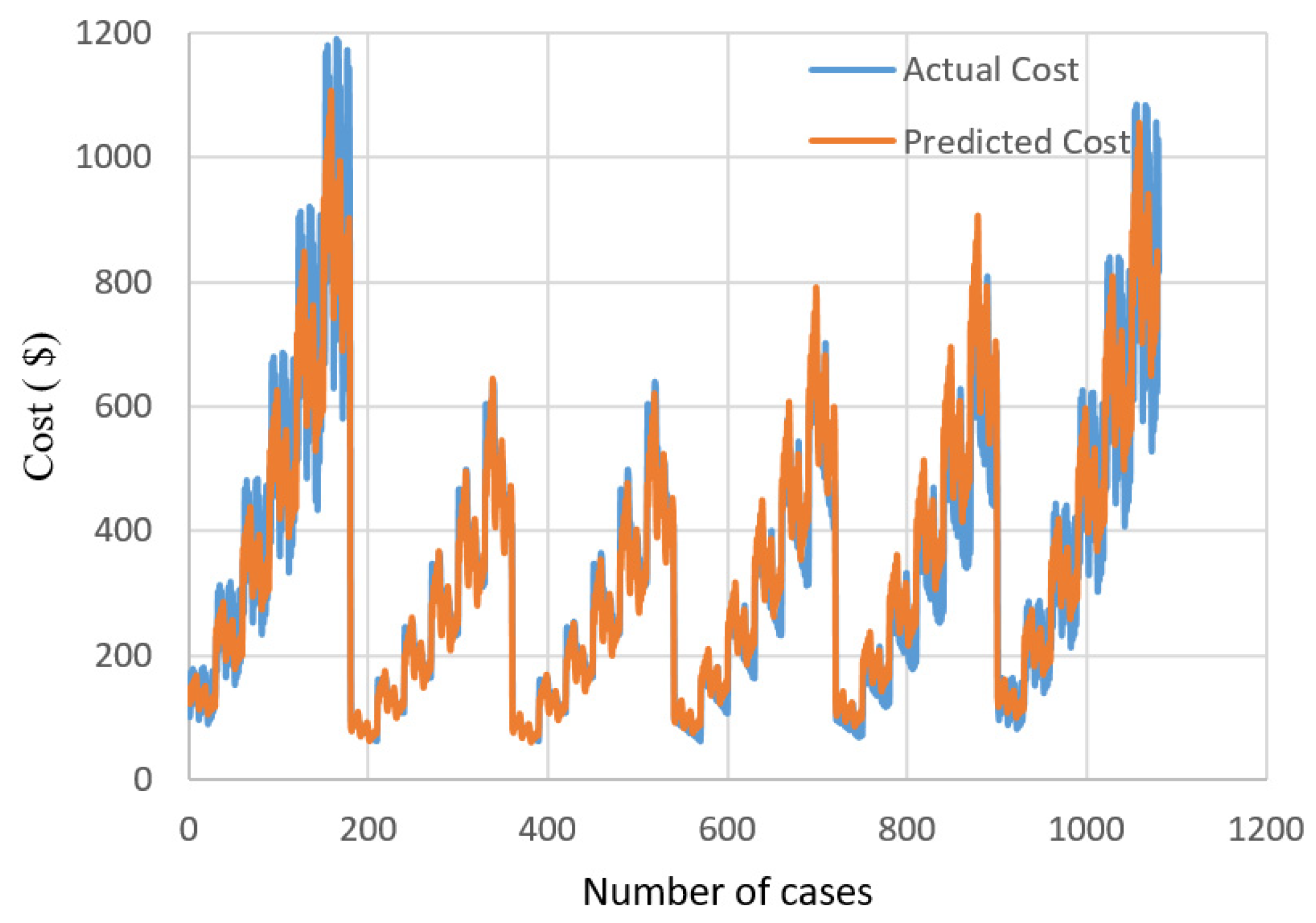
Figure 4.
Comparison of actual and predicted costs.

Figure 5.
Actual and predicted costs versus number of cases for validation.

Figure 6.
Comparison of actual and predicted costs for validation.


Table 1.
Recommended preliminary dimensions for RC cantilever walls in different references.
| Reference | a | b | B |
|---|---|---|---|
| TS 7994 [27] | 20–30 cm | 0.33B | 0.4H–0.7H |
| ACI 318 [28] | 8–12 inch | 0.33B | 0.4H–0.6H |
| Bowles [26] | 20–30cm | 0.33B | 0.4H–0.7H |
Table 2.
Input parameters.
| Input Parameters | Data |
|---|---|
| Height of the wall (H) | 3, 4, 5, 6, 7, and 8 m |
| Slope of the backfill (β) | 0°, 10°, 15°, 20° and 25° |
| Inclination of the back of the stem with respect to the horizontal axes (Ψ) | 90° |
| Angle of friction between cantilever wall and backfill soil (δd) | 0° |
| Internal friction angle (Φd) and unit weight (γd) of backfill | 30°, 18 kN/m3; 35°, 19 kN/m3; 40°, 18 kN/m3 |
| Depth of soil in front of the wall (D) | 1 m |
| Internal friction of foundation soil (Φ2) | 25° |
| Cohesion of foundation soil (c2) | 70 kPa |
| Undrained shear strength of foundation soil (cu) | 250 kPa |
| Soil site class | ZC |
| Reduction coefficient for internal friction angle between foundation soil and RCCRW (k1) | 0.88 |
| Reduction coefficient for cohesion between foundation soil and RCCRW (k2) | 0.55 |
| Allowable bearing capacity of the soil (qall) | 800 kPa |
| Design bearing capacity of the soil (qt) | 1600 kPa |
| Design earthquake spectral response acceleration parameter at short periods (SDS) and locations | 0.419 (Konya), 0.447 (Ankara), 0.646 (Antalya), 0.845 (Erzurum), 1.184 (Kahramanmaraş), 1.333 (İzmir) |
| Equivalent static earthquake reduction coefficient (r | 1.5 and 2.0 |
| Compressive strength of concrete | 30 MPa |
| Unit weight of the concrete | 24 kN/m3 |
| Yield strength of steel | 420 MPa |
Table 3.
Design constraints.
| Design Constraints | Failure Mode |
|---|---|
| Overturning check (static) | |
| Sliding check (static) | |
| Bearing capacity check (static according to allowable stress design) | |
| Bearing capacity check (static according to allowable stress design) | |
| Overturning check (seismic, vertical component of seismic loading in upwards direction) | |
| Overturning check (seismic, vertical component of seismic loading in downwards direction) | |
| Sliding check (seismic, vertical component of seismic loading in downwards direction) | |
| Bearing capacity check (static according to TBDY [23] with 1.4 G* + 1.6 H* load combination) | |
| Bearing capacity check (static according to TBDY [23] with 1.4 G + 1.6 H load combination) | |
| Bearing capacity check (static according to TBDY [23] with 0.9 G + 1.6 H load combination) | |
| Bearing capacity check (static according to TBDY [23] with 0.9 G + 1.6 H load combination) | |
| Bearing capacity check (seismic according to TBDY [23] with G + H + E* load combination) | |
| Bearing capacity check (seismic according to TBDY [23] with G + H + E load combination) |
*G, H and E are dead load, horizontal load due to lateral earth pressure and earthquake load, respectively.
Table 4.
Basic prices used in the present study.
| Cost of reinforcement (Creinforcement) | 0.38 USD/kg |
| Cost of concrete (Cconcrete) | 32.0 USD/m3 |
| Cost of backfill (Cbackfill) (Φd = 30°; γd= 18 kN/m3) | 17.5 USD/m3 |
| Cost of backfill (Cbackfill) (Φd = 35°; γd= 19 kN/m3) | 18.0 USD/m3 |
| Cost of backfill (Cbackfill) (Φd = 40°; γd= 18 kN/m3) | 18.5 USD/m3 |
Table 5.
Lower and upper bounds of design variables.
| Design Variable | Lower Bound (m) | Upper Bound (m) |
|---|---|---|
| a (width of the stem at the top) | 0.2 | 0.3 |
| b (toe part of the base) | 0.10 H | 0.231 H |
| c (width of the stem at the bottom) | 0.08 H | 0.1 H |
| d (heel part of the base) | 0.08 H | 0.1 H |
| h (thickness of the base) | 0.07 H | 0.10 H |
| D′ (height of the base shear key) | 0 | 2 |
Table 6.
Utilized data for the validation.
| Input Parameters | Data |
|---|---|
| Height of the wall (H) | 3.5, 4.5, 5.5, 6.5 and 7.5 m |
| Slope of the backfill (β) | 12.5°, 17.5° and 22.5° |
| Inclination of the back of the stem with respect to the horizontal axes (Ψ) | 90° |
| Angle of friction between cantilever wall and backfill soil (δd) | 0° |
| Internal friction angle (Φd) and unit weight (γd) of backfill | 30°, 18 kN/m3 35°, 19 kN/m3 40°, 18 kN/m3 |
| Depth of soil in front of the wall (D) | 1 m |
| Internal friction of foundation soil (Φ2) | 25° |
| Cohesion of foundation soil (c2) | 70 kPa |
| Undrained shear strength of foundation soil (cu) | 250 kPa |
| Soil site class | ZC |
| Reduction coefficient for internal friction angle between foundation soil and RC cantilever wall (k1) | 0.88 |
| Reduction coefficient for cohesion between foundation soil and RC cantilever wall (k2) | 0.55 |
| Allowable bearing capacity of the soil (qall) | 800 kPa |
| Design bearing capacity of the soil (qt) | 1600 kPa |
| Design earthquake spectral response acceleration parameter at a short period (SDS) and locations | 0.419, 0.447, 0.646, 0.845, 1.330 and 1.1840 |
| Equivalent static earthquake reduction coefficient (r | 1.5 and 2.0 |
| Compressive strength of concrete | 30 MPa |
| Unit weight of the concrete | 24 kN/m3 |
| Yield strength of steel | 420 MPa |
Disclaimer/Publisher’s Note: The statements, opinions and data contained in all publications are solely those of the individual author(s) and contributor(s) and not of MDPI and/or the editor(s). MDPI and/or the editor(s) disclaim responsibility for any injury to people or property resulting from any ideas, methods, instructions or products referred to in the content. |
© 2023 by the author. Licensee MDPI, Basel, Switzerland. This article is an open access article distributed under the terms and conditions of the Creative Commons Attribution (CC BY) license (https://creativecommons.org/licenses/by/4.0/).
Share and Cite
MDPI and ACS Style
Akis, E. Optimum Cost Prediction of Reinforced Concrete Cantilever Retaining Walls. Buildings 2023, 13, 2409. https://doi.org/10.3390/buildings13102409
AMA Style
Akis E. Optimum Cost Prediction of Reinforced Concrete Cantilever Retaining Walls. Buildings. 2023; 13(10):2409. https://doi.org/10.3390/buildings13102409
Chicago/Turabian StyleAkis, Ebru. 2023. "Optimum Cost Prediction of Reinforced Concrete Cantilever Retaining Walls" Buildings 13, no. 10: 2409. https://doi.org/10.3390/buildings13102409
Note that from the first issue of 2016, this journal uses article numbers instead of page numbers. See further details here.