
Study of Damping of Bare and Encased Steel I-Beams Using the Thermoelastic Model


CIMOSM, ISEL—Centro de Investigação em Modelação e Optimização de Sistemas Multifuncionais, Instituto Politécnico de Lisboa, 1959-007 Lisboa, Portugal
Buildings 2023, 13(12), 2964; https://doi.org/10.3390/buildings13122964
Submission received: 18 September 2023
/
Revised: 19 November 2023
/
Accepted: 24 November 2023
/
Published: 28 November 2023
(This article belongs to the Special Issue Novel Computational and Numerical Methods for the Analysis of Solids and Structures)
Abstract
:Steel I-beams are a fundamental structural component in civil construction. They are one of the main load-bearing components in a building that must withstand both the structure and any incoming external perturbations, such as seismic events. To avoid damage to the structure, the building must be designed to dissipate the maximum amount of energy possible. One way energy can be dissipated is through internal or structural damping, of which thermoelasticity is one of the causes, especially in low-frequency harmonic excitations. The main goal of this study is to analyze the amount of damping in an I-beam generated by thermoelasticity and when encased in a Portland cement concrete layer, using a Finite Element model. It was found that, due to the geometry of the I-Beam, the damping coefficient as a function of frequency has two local maxima, as opposed to the traditional single maximum in rectangular beams. Encasing an I-beam in a concrete layer decreases the overall damping. While the extra coating protects the beam, the reduction in damping leads to a lower energy dissipation rate and higher vibration amplitudes.
1. Introduction
Seismic events are low-frequency, high-energy events that can impart heavy structural damage on structures [1,2,3,4]. The energy propagating through the soil into the structure can be partially dissipated rather than converted into deformation. Several strategies exist to maximize damping, either through deliberate design of stationary structures and materials [5,6,7,8,9], or via the employ of dynamic absorber devices (active or passive) which make use of moving parts to counter-balance incoming vibrations [10,11,12]. On the other hand, natural dissipation phenomena are always present in any structure. Macroscopically, they originate from the friction between bolted or riveted parts. Microscopically, the main damping phenomenon is structural damping [13,14,15]. Structural damping is an umbrella term that includes all damping sources intrinsic to a solid structure and excludes damping due to viscous interaction with a fluid or direct friction with another moving part [13].
Since the source of structural damping is not unique [13], several models have attempted to predict the dynamic behavior of a structure. One of the most well-known models is the hysteretic model [13,16,17,18,19]. This model, however, causes controversy in the scientific community. The consensus is that this model can only be used in the analysis of steady-state vibrations because of the supposed non-causality of the transient response [16,18,20,21,22,23,24]. In actuality, this model has trouble modeling the transient response due to an unstable differential equation. Therefore, a more generic model is needed to cover both regimes. Fractional derivative models are also common in the study of structural damping, especially in polymeric materials [19,25,26,27,28]. However, these are empirical models which share a significant drawback: there is no single definition for fractional derivatives. A commonly overlooked alternative is the thermoelastic model.
The thermoelastic model is derived from first principles and fully couples the elastic wave equation with the heat equation. While the origins of this model can be traced back to the 1950s [29,30], because of its complexity, only with the advent of modern computers could this model be more thoroughly exploited [30,31,32,33,34,35]. This model simulates damping phenomena at the micro-scale [36,37,38,39], since that effect is more pronounced in smaller structures. However, it is also noticeable in larger structures at lower frequencies [35,40]. Since seismic events tend to occur in the lower band of the frequency spectrum, thermoelasticity could contribute significantly to the overall damping. This paper compares the thermoelastic damping behavior of concrete-encased steel I-beams to that of bare beams. Steel I-beams are fundamental structural elements used in buildings and, together with columns, are their main load-bearing components. Understanding the dynamic behavior of these elements, especially in what damping is concerned, can help engineers design structures that are better prepared to handle incoming dynamic loads. While there have been several studies on thermoelasticity applied to beams or plates (either “regular” size or micro/nano-sized), most sources have focused on the study of elements with rectangular cross-sections [30,31,32,33,36,37,38,39,41,42].
The case studies presented in this work focus on beams under a bending load, and the analysis uses solid elements instead of the more common beam elements [30,32,33,39]. Since solid elements are more versatile, the variation of temperature across the thickness of the beam can be studied in more detail. The main disadvantage is that solid elements are computationally more expensive since the analysis requires more elements than it otherwise would in order to capture bending behavior accurately.
The article is divided into four main sections: Introduction, Materials and Methods, Results and Discussion, and Conclusions. The thermoelastic model differential equations are presented in the Materials and Methods section. This section also covers the formulation of the 3D hexahedral element and the nuances in its use in conjunction with the thermoelastic model (e.g., boundary conditions). In the Results and Discussion section, the model validity is assessed, mesh generation and convergence studies are performed, and the results of the simulations are presented.
2. Materials and Methods
2.1. The Thermoelastic Model
The thermoelastic model or linear thermoelasticity dynamic model results from the complete coupling of the elastic wave equation with the heat equation and is given by (1):
where is the displacement vector (), is the temperature variation, f is the body load and q is the body heat flux. All function quantities are functions of the Euclidean coordinates and time. The constants in the model are the material properties: density (), Lamé constants ( and ), specific heat capacity (), and thermal conductivity (k).
The Lamé constants are given by:
where E is the Young modulus and is the Poisson coefficient.
Since temperature is critical to the problem, all coefficients must be specified at the same base temperature , the point around which linearization is performed in the thermoelastic model. Finally, the coefficient is the coupling term and is given by:
where is the linear thermal expansion coefficient. Since Equation (1) is a linearized equation, it is only valid for small deformations and small temperature variations: .
The coupling term in the elastic wave equation is and results from the thermal strain in elastic materials:
where is the strain generated by temperature variation and is the Kronecker Delta. The total strain, is given by:
where is the mechanical strain (stress-induced strain).
The coupling term in the heat equation is and is the result of the definition of entropy:
where s is the specific entropy and is the total strain. A more detailed demonstration of the coupling term in the thermal equation can be seen in [29].
2.2. Energy Flow and Balance in the Thermoelastic Model
Because it couples two fields in a single system, the thermoelastic model has some particularities regarding energy flow, especially when compared with the standard elastic wave equation. Analyzing the energy flow makes it possible to understand the phenomena behind the damping predicted by this model. A complete representation of the energy flow in the system can be seen in Figure 1.
The conservative energies are the potential energy (), kinetic energy () and exergy (), which are given by Equation (7):
The only non-conservative energy in the domain is the work lost to irreversible entropy generation. One of the characteristics of the Equation (1) is that the damping term is not explicit, much unlike all other damping models used in mechanical vibrations. Damping occurs by generating irreversible Entropy due to the existing internal heat fluxes. The irreversible entropy is generated whenever there is a heat flux in the material, and the total energy lost this way is given by the Gouy-Stodola theorem [31]:
where is the work lost to irreversible entropy.
Internal entropy generation is not the only way the system can lose energy. Energy can also be lost through the boundaries either by imposing a fixed temperature, imposed nonzero flux, or through convection. When the system is thermally open, the entropy can flow into and out of the domain due to the generated heat fluxes. These boundary fluxes are the Work (Equation (9a)) and Heat (Equation (9b)):
In light of the First Law of Thermodynamics, the complete energy balance is given by the following equation:
where is the variation of the internal energy. In this energy balance, the work done on the system is positive.
If the study is focused on harmonic analysis, then all conservative energies in a cycle are zero, and, as such, the Equation (10) reduces to:
In this study, all thermal boundary conditions are Adiabatic, and the heat transferred () is always zero. The dissipated energy can be determined either by Equation (9a) or Equation (8) since they have to be equal. However, the dissipated work is not a very good measure of the damping of a system since it is susceptible to the presence of resonances and, as such, is not generic or comparable enough. An alternative is to use the loss angle or an equivalent damping factor.
The loss angle is a quantity widely used in material science to characterize damping in viscoelastic materials and is the phase of a complex Young modulus definition:
where is the dynamic modulus, is the storage modulus (reduces to the Young Modulus in purely elastic materials), is the loss modulus that quantifies the dissipated elastic energy, and is the loss angle.
The loss angle is related to the hysteretic model and the hysteretic damping coefficient:
where is the hysteretic damping coefficient.
For the hysteretic model, the damping coefficient can be extracted from the work made by a load using the maximum elastic potential energy:
where k is the stiffness of the spring, and X is the complex amplitude of the displacement. The denominator of Equation (14) is the maximum potential energy in a cycle. The equivalent hysteretic damping coefficient is also known in the literature as the quality factor () (The TED under script refers to the thermoelastic damping. The Quality Factor can be defined for any damping) [40,43,44].
2.3. Finite Element Model
The thermoelastic model was implemented on an in-house Finite Element Analysis software in 2D quadrilateral and 3D hexahedral solid elements (linear and quadratic for 2D and linear for 3D). The software was written in C++ and Intel® Math Kernel Library performs the linear algebra routines. All elements support static, dynamic, and harmonic analysis.
For this study, a solid linear hexahedral 3D element was defined according to the Figure 2.
For the given reference frame, the shape functions are given by Equation (15):
where are the shape functions and u, v and w are the element internal coordinates that are in the interval .
To determine the element matrices, the weak form of Equation (1) must be determined. The first step is to expand the differential operators and explicitly write the equation as a system of four differential equations:
where , and are the displacements in the x, y and z directions, respectively. As represented in Equation (16), the system has three elasticity equations and one thermal equation. The discretization process for the displacements and temperature variations is explained in detail in Appendix A.
After the discretization process is done, Equation (A4) can be joined with Equations (A11a), (A11b) and (A14) and the full discretized system is given by:
where , and , are the mass, velocity (the term damping matrix should be avoided because the damping in the thermoelastic model is not completely contained in this matrix) and stiffness matrices, given by:
It is important to note that while Equation (17) is written with second-order derivatives, the system is, in fact, a third-order system (this can be seen in the mass matrix, which is non-invertible). Also, Equation (17) can be applied to a single element or the entire mesh, assuming each matrix is correctly assembled.
2.4. Boundary Conditions
Boundary conditions (BC) are a fundamental component of boundary value differential equation problems, sometimes overlooked. While the boundary conditions for individual problems in Elasticity and Heat conduction are well-studied, their coupling generates new boundary conditions with unique properties. These conditions must be explicitly presented, particularly in the case of Neumann boundary conditions (Neumann BCs).
Neumann BCs are conditions proportional to the gradient of displacements (or temperature variation). In classical Elasticity, they are employed to incorporate any applied forces into the system at the boundaries of the structure. In heat problems, Neumann BCs are used to introduce external heat fluxes.
Using a 1D example for simplicity, a Neumann BC for the Elasticity problem is:
where E is the material Young Modulus, A is the area of the boundary, P is the distributed load applied at the boundary and is the boundary.
When using the thermoelastic model, according to Equation (5), the strain not only depends on the applied force (similarly to Equation (19)) but also on the temperature variation. As such, the BC in Equation (19) has to be updated to include the temperature variation, becoming:
This new boundary condition is pivotal to the model as it addresses a seemingly paradoxical behavior inherent in thermoelasticity under adiabatic conditions:
- When a body is stretched, it cools down, and when compressed, it heats up.
- When heated, a body expands, and when cooled, it shrinks.
The first behavior is embedded in the differential equations themselves, whereas the second behavior is represented by the boundary condition in Equation (20).
The seemingly minor modification described above has profound implications for both the problem and the subsequent finite element model. Firstly, as evident from Equation (20), the thermoelastic model exhibits not Neumann boundary conditions (BCs) but rather Robin BCs. This distinction arises because the BC is a linear combination of the first derivative of a state (displacement, ) and a state ().
The second consequence pertains to the finite element implementation, compelling the analysis to consider all boundaries, even those without externally applied loads.
The third implication arises when multiple materials are employed on a mesh, as exemplified in the case of a concrete-encased beam. In classical elasticity and heat conduction problems, a finite element model mesh can accommodate multiple materials without special modification, provided that individual elements maintain a single material. This accommodation is feasible due to the continuity of forces inside the mesh, extending across material boundaries. In contrast, when transitioning to the thermoelastic model, only internal forces remain continuous. The final monomial in Equation (20) introduces discontinuity (This term behaves akin to a fictitious force, contingent upon the material properties and temperature variation). Consequently, in the thermoelastic model, internal boundaries need to be added at material interfaces within the mesh. For a 1D problem, this scenario is depicted in Figure 3.
As seen in Figure 3b, while the internal force (f) is in balance, the “thermal forces” are not, and an imbalance generates a net force. If the standard implementation of a finite element model is used, this imbalance is ignored, leading to incorrect results.
Implementation of the Boundary Conditions
The hexahedral thermoelastic solid element has six boundaries, identified in Figure 4.
A series of boundary terms appeared when performing the integration by parts on Equation (A2). These terms are:
According to Equation (20), the boundaries terms defined in Equation (22) are also:
where is the x coordinate of the distributed load applied on the surface of the boundary and is the x coordinate of the normal vector of the given boundary.
Applying the discretizations in Equation (A3) and a similar one to Equation (A6), the discretized boundary terms are:
The matrices are the boundary matrices and are similar to Equation (A5a), but only integrated at the assigned boundary:
The matrices are the boundary matrices with the x coordinate of the normal vector:
As with body loads, the computational cost of integrating loads and temperature variations at boundaries is considerably reduced through the use of boundary matrices. However, in the context of Equation (25), it is crucial to exercise caution to prevent a substantial normal rotation. Should the problem result in a significant rotation of the boundary normal, it becomes imperative to update these matrices during the simulation.
Finally, the element matrices in Equations (24) and (25) are not assembled like the other element matrices. Instead, they are only assembled for elements at the structure boundaries and using only the boundary matrices corresponding to the exposed element sides.
With the boundaries defined, the boundary term, , in Equation (17) is defined as:
where is the number of boundaries in the mesh added to any internal boundary generated by a material interface.
2.5. Harmonic Solution
To get the solution of the harmonic problem, a Fourier transform must be applied to Equation (17):
where is the angular frequency of the excitation and , , , , and are the complex amplitudes of the displacements, temperature variation, body forces, body heat fluxes, boundary loads and boundary heat fluxes, respectively. The matrix contains the Robin BC elements of the thermoelastic BCs:
Finally, to apply Dirichlet BCs, the system matrix must be decoupled accordingly.
To obtain the complex amplitudes (and the corresponding amplitudes and phases), Equation (27) is solved using the linear equation solver.
2.6. Energy Computation in the Finite Element Model
For a harmonic analysis, as stated by Equation (11), only the boundary energy fluxes and the work lost to irreversible Entropy need to be determined. To determine these quantities used the finite element model, Equations (8), (9a) and (9b) must be discretized and integrated for a complete cycle ()
The discretized Gouy-Stodola theorem for a cycle is given by:
where .
To compute the work and heat transfer in a cycle, the nodal loads must be determined first. Due to the Dirichlet BCs (direct imposition of values of DoFs), reaction loads (forces and heat fluxes) are generated in response. To determine these loads, the input vector (the right side of Equation (27)) has to be recomputed:
The quantities with the “node” subscript are the nodal loads, and the system matrix is the full matrix without decoupling.
With the nodal loads, the work and heat in a cycle are given by:
Note that for Equations (29) and (31b), if , both equations result in an indeterminate form. This indeterminate form can be lifted by computing the limits, which always yields zero for both equations.
Finally, the equivalent hysteretic damping coefficient is determined by:
2.7. Geometries and Materials
In this work, two geometries are studied, a symmetrical ASTM A6 wide flange I-beam (W150 × 100 × 24.0, Figure 5a and Table 1) bare or completely encased (Figure 5b).
The length of all beams in this study is , guaranteeing a length/height ratio 10. Two thicknesses of the encasing () were used: and .
Apart from one case study, where the beam is made of copper, all case studies use standard steel (for more information on the case studies, please refer to Section 3.3). For the casing, on the encased studies, it was used an average Portland cement concrete (28 days cure). The material properties can be seen in Table 2. For all properties, the base temperature, , is .
3. Results and Discussion
3.1. Validation Study
During the literature review, no published results were found for damping I-beams. The thermoelastic model has been extensively validated previously; for example, Zener compared the predicted maximum quality factor for different rectangular beams [43]. More recently, Zuo et al. compared the numerical simulation of a double-clamped quartz micro-beam, showing a good fit with the experimental data [41].
A study using a double-clamped rectangular beam in [40] was replicated to validate the developed element. The validation study is also compared with base benchmarks using similar analyses done by Zener [43] and Lifshitz and Roukes [44].
The geometry used in the validation is a double-clamped rectangular beam with a length (L) of and a width (b) of ; the thickness (h) varies throughout the study, Figure 6.
The objective of the authors in Parayil et al. [40] was to study the evolution of the quality factor (the equivalent hysteretic damping coefficient) at the first bending mode, with an increasing beam thickness by using different implementations of a Timoshenko-based thermoelastic model. The material used in the simulations was silicon with the properties in Table 3.
The comparative results are shown in Figure 7.
The present study (SLD-FEM) matches the Thimoshenko-based model (TBT-A1) results for all thicknesses. The study also fits well with the results obtained by Zener (EBT-Z) and Lifshitz (EBT-LR) for more slender beams, which is expected since both analyses rely on an Euler-Bernoulli beam model.
The mesh used in the SLD-FEM study varies since the thickness also changes. After a convergence study for each case, the final mesh has 220 elements across the length and 19 elements across the width. The number of elements across the thickness, , is given by the following expression:
where h is the thickness of the beam.
3.2. Mesh Convergence
Only two geometries were used in this study: the bare I-beam and the encased I-beam, and, as such, only two meshes were used. The implementation of the solid element was validated against standard cases for the elastic model.
To determine the mesh parameters, a mesh convergence study was done for both meshes. Since, in this article, only harmonic simulations are used, the convergence of the first two natural frequencies was chosen as the convergence criterion.
For simplicity, the mesh parameters were defined as a function of the number of elements across the length of the beam ():
For the encased I-beam, the number of elements in the casing thickness () is given by:
3.3. Case Studies
For this article, nine different case studies were used. The description of all cases can be seen in Table 6.
All case studies use a beam with a 10:1 ratio to the total height of the I-beam (10 H), and all cases use a distributed load applied at , Figure 10. The position of the force was chosen to avoid nodes in the bending mode shapes, guaranteeing that the maximum vibration modes are excited.
Regarding the BCs, all case studies feature double-clamped beams (at and ), and all boundaries are Adiabatic.
Adiabatic boundaries signify that the model enforces no heat flux at any boundary. Other potential boundary conditions include the imposition of temperature (Dirichlet), convection (Robin), and radiation (non-linear BC), each influencing the damping characteristics of the beam. The imposition of a constant temperature is unrealistic, assuming surfaces maintain a constant time-controlled temperature. Physically, this would require the application of temperature-controlled heaters on all surfaces, essentially creating a thermal clamp. Conversely, convection and radiation boundary conditions are more realistic. Convection represents heat transfer between a solid and a fluid (or vice versa) and is modeled by Newton’s law of cooling. However, in terms of damping, this law has no impact as it assumes the surrounding fluid is inviscid, resulting in no energy dissipation under harmonic excitation [35]. Realistic convection studies necessitate modeling the structure-fluid interaction, which is computationally expensive and minimally impactful since natural air convection is overshadowed by conduction in this study. Consequently, it is approximated by imposing adiabatic BCs. The energy lost through radiation is even smaller, particularly considering that beams in buildings are typically not directly exposed to solar radiation, and inter-surface radiation indoors is negligible.
In the case of encased beams, case studies SI018 and SI019 mirror SI009 and SI012, respectively, but employ a single theoretical volume-mixed material instead of the two material phases. This theoretical material results from a volume-weighted average of steel () and Portland cement concrete () properties. These studies aim to discern the influence of geometric material phase distribution on results, determining if one-dimensional beam elements suffice. If volume-mix results align with two-phase case studies, solid elements become unnecessary, and computationally less expensive beam elements are preferable.
The concrete casing thickness of adheres to standard civil construction practices and represents the maximum thickness allowed by the Eurocode.
3.4. Harmonic Behavior of I-Beams
The thermoelastic model is more prominent in low frequencies; as such, all case studies were run in two frequency sweeps: a long-range “low” resolution sweep from 0 to with a resolution of and a short-range variable high-resolution frequency sweep from 0 to . The first sweep was done to understand how the model behaves in a broader range and compare it with the other models. The second sweep is more focused on representing the evolution of the equivalent damping coefficient with frequency.
The long-range frequency sweep Bode diagram for the first three case studies is shown in Figure 11.
The Bode diagram shown in Figure 11 was taken on the line of the applied load (Figure 10) at the center of the beam (y direction). The three case studies show the comparison between the standard elastic model (SI001), the hysteretic model (SI002, with ), and the thermoelastic model (SI003), Table 6. All models show nearly coincident resonant frequencies but very different behaviors in damping (more evidently in the phase). The first two resonant frequencies for the three models are shown in Table 7.
The Bode diagram, depicted in Figure 11, was captured along the line of the applied load (Figure 10) at the beam center in the y-direction. The comparison across three case studies, as illustrated in Table 6, includes the standard elastic model (SI001), the hysteretic model (SI002) with a damping ratio of , and the thermoelastic model (SI003). Although all models exhibit nearly coincident resonant frequencies, they manifest distinct damping behaviors, particularly evident in the phase. The first two resonant frequencies for each model are summarized in Table 7.
In terms of temperature distribution, a reasonable interpretation can be made using the first mode shape of the beam, Figure 12a (the values at the axis do not have the physical meaning as the actual displacements depend on the initial conditions). The cross-section at the anti-node can be seen in Figure 12b.
As expected, the beam cools down on the traction side and heats at the compression side of the beam. The temperature variation is smooth across the cross-section, except for some concentration at the interfaces between the flanges and the web.
Using Equation (32), the behavior of the equivalent damping coefficient for the I-beam thermoelastic case studies (SI003 and SI004) is shown on Figure 13.
The overall behavior closely aligns with anticipated thermoelastic patterns, as demonstrated in previous works [34,35,45]. As anticipated, the copper beam exhibits higher damping than steel, primarily attributable to the superior thermal conductivity of copper relative to steel.
The occurrence of maximum damping corresponds to excitation frequencies aligning with the inverse of a time constant in the thermal equation [40]. However, as depicted in Figure 13, two distinct maxima are observable, particularly pronounced in the copper case study. One plausible explanation for this phenomenon lies in the use of 3D solid elements on a relatively thick beam, revealing more complex behaviors compared to conventional one-dimensional beam elements found in literature [32,34,45]. Additionally, the I-beam shape introduces two thicknesses—the web and flange—with comparable dimensions, bringing the first two thermal time constants into closer proximity.
3.5. Harmonic Behavior of Encased I-Beams
Two frequency sweeps were also done in the encased I-beam simulations (case studies SI009 to SI012, Table 6). However, the “low” resolution sweep was done with a different range: 0 to . The simulation of the thermoelastic model is considerably more expensive, computationally, than the elastic model. Since this work focuses on lower frequencies, a range that only captures the first mode of vibration was chosen. The first frequency sweep Bode diagram is shown in Figure 14.
As evident from Table 7 and Table 8, the resonant frequency of the thermoelastic model is consistently higher than the natural frequency of the elastic model. This observation may initially seem counterintuitive, as damping typically decreases the resonant frequency in comparison to an undamped system. However, the thermoelastic model introduces unique characteristics related to the Heat equation.
Recalling the energy balance in a thermoelastic system, illustrated in Figure 1 and governed by Equations (7) and (8), the Heat equation introduces, alongside damping, the concept of Exergy. Exergy serves as an additional energy storage mechanism, quantifying the potential of temperature imbalances. Since the squared natural frequencies of a system are proportional to the ratio between potential energies and kinetic energy, an increase in the former results in higher natural frequencies. This phenomenon arises because the Heat equation lacks a “thermal inertia” term.
The absence of “thermal inertia” has been a topic of discussion in the scientific community [46,47,48,49], primarily because Fourier’s Law predicts instantaneous excitation propagation throughout the domain. While acceptable in Classical Physics, this contradicts Modern Physics, which asserts that no phenomena can travel faster than the speed of light.
In the Classical Thermodynamics context, Fourier’s Law remains a viable approximation because thermal conduction phenomena are “very slow” relative to the speed of a hypothetical thermal wave, and the “thermal inertia” is likely orders of magnitude smaller compared to the conduction term, allowing it to be safely disregarded. However, when coupling the Heat equation with other equations predicting faster phenomena, such as the Wave Equation, neglecting “thermal inertia” could lead to deviations. Unfortunately, reliable values for proposed “thermal inertias” for the materials used could not be found during the research for this work.
The distribution of the temperature variation in the cross-section of the encased beam (for the case studies SI012 and SI019, at the resonance) can be seen in Figure 15.
By comparing Figure 15b,d, the impact of two material phases on temperature distributions becomes evident. The temperature profile for the volume mix closely resembles that of case study SI003 (Figure 12b), displaying a gradual transition from colder regions (under tension) to hotter regions (under compression). However, when examining the results of case study SI012, where distinct material phases are present, the temperature distribution is no longer smooth. In this instance, a noticeable disparity emerges between the temperature profiles of the two material phases. Specifically, the central I-beam exhibits a higher temperature variation than the surrounding concrete casing. This discrepancy emphasizes that the material phase distribution is a crucial factor that cannot be overlooked, rendering the use of one-dimensional beam elements inadequate.
The computation of the evolution of the equivalent damping coefficient for the encased case studies is illustrated in the plot presented in Figure 16.
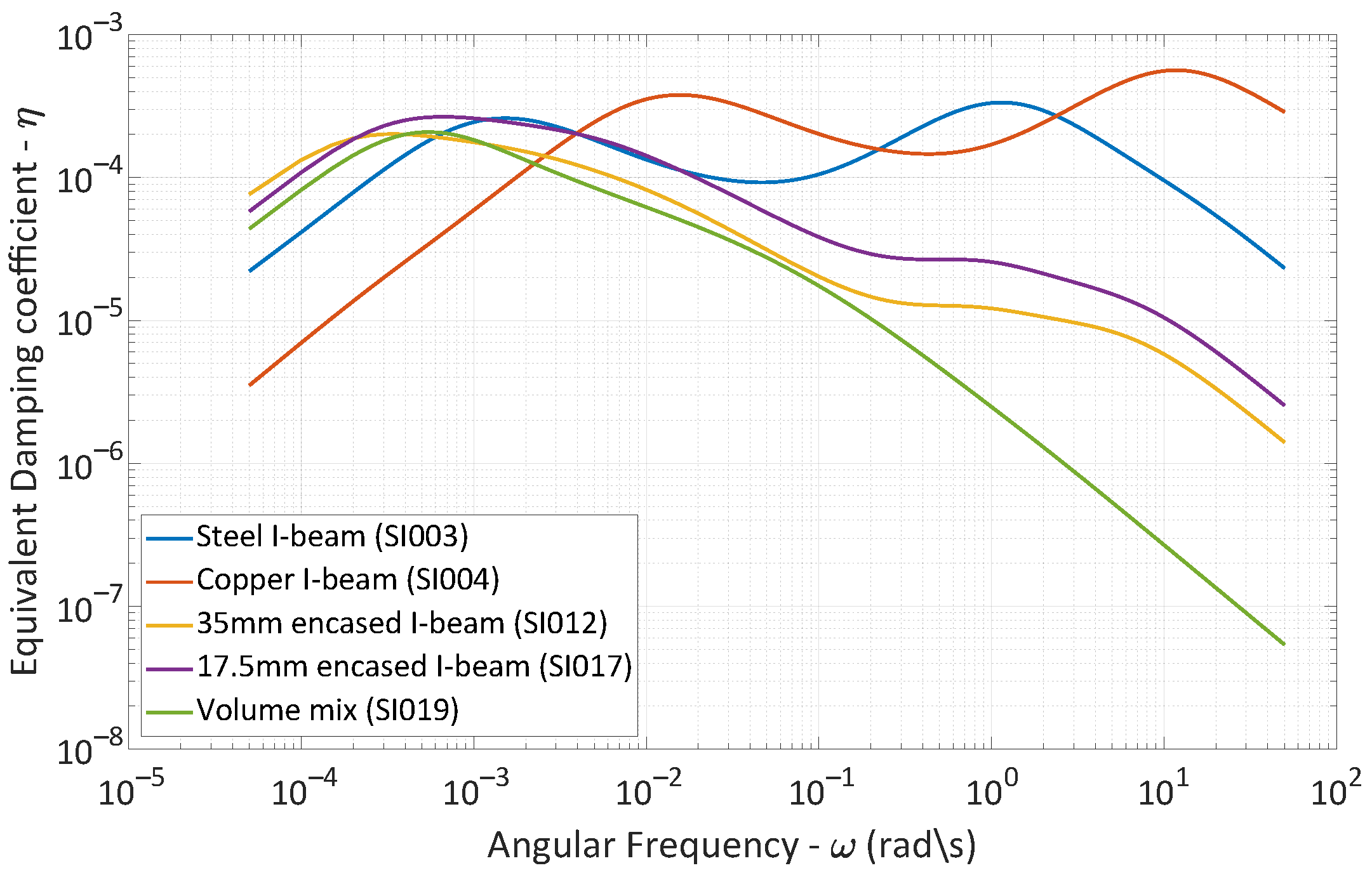
The first observation one can take from Figure 16 is the overall decrease in the frequency of the maximum point. The damping values also decrease significantly in all frequencies. A better comparison between all case studies can be seen in Figure 17 by plotting the damping coefficients in a log-log scale.
The decrease in the thermoelastic damping coefficient between the cased and bare I-beams can be attributed to two key characteristics of the model and geometry. Firstly, thermoelastic damping is typically higher in thin geometries where temperature variations are more pronounced, resulting in higher energy losses. The addition of a thick casing substantially increases the overall bulk of the beam, mitigating the impact of the I-beam’s thin features. Secondly, heat conduction is more effective than convection (assumed to be nearly adiabatic in this study). Despite having a smaller thermal conduction value than steel, the concrete layer diffuses temperature variations across its section. This diffusion significantly diminishes temperature gradients, following the Gouy-Stodola theorem (Equation (8)), thereby reducing the energy lost to irreversible temperature generation. When halving the casing thickness (as observed in case study SI017), the damping decrease is less pronounced, and within a certain frequency interval, it becomes comparable to that of the bare I-beam.
4. Conclusions
This study primarily aimed to investigate the damping of bare and concrete-encased I-beams due to the inherent thermoelastic effect. The results obtained from simulations using harmonic Finite Element Analysis reveal the following:
- The thermoelastic model predicts an increase in the resonant frequencies, potentially attributable to the absence of “thermal inertia” in Fourier’s Law.
- A steel I-beam exhibits a maximum damping coefficient of , and due to the cross-section geometry of the beam, the damping evolution with frequency demonstrates two local maxima.
- The addition of a concrete casing to the I-beam reduces the maximum damping coefficient (approximately ), indicating that the beam dissipates less energy due to thermoelasticity compared to the bare configuration.
- While the added layer protects the beam, the decreased damping value results in less energy dissipation and a slower reduction in vibration amplitude.
- Given the distinct behavioral differences across the beam cross-section between the two material phases in case study SI012, traditional one-dimensional beam elements should not be employed, as they would oversimplify the problem.
This study prompts several questions for future research. Foremost is the imperative to experimentally validate the obtained results under controlled conditions. The model developed for this study can assist in designing the experiment and selecting suitable sensors and actuators. Another question to be explored in future work is the increase in resonant frequencies due to the absence of “thermal inertia” in the heat equation. The speed of the hypothetical thermal wave (or “second sound”, as termed by some authors) should be studied for the materials used in this investigation to refine and update the thermoelastic model.
Funding
This research received no external funding.
Data Availability Statement
Data are contained within the article.
Conflicts of Interest
The author declares no conflict of interest.
Abbreviations and List of Symbols
| The following abbreviations are used in this manuscript: | |
| DoF | Degree of Freedom |
| BC | Boundary Condition |
| The following symbols are used in this manuscript (in order of appearance): | |
| Density | |
| Displacement vector | |
| Second Lamé constant | |
| First Lamé constant | |
| Thermoelastic coupling coefficient | |
| Temperature variation | |
| f | Volumetric load |
| Specific heat capacity | |
| k | Thermal conductivity |
| Base temperature | |
| q | Volumetric heat flux |
| Poisson coefficient | |
| E | Young modulus |
| Thermal expansion coefficient | |
| Thermal strain | |
| Kronecker Delta | |
| Total strain | |
| Mechanical strain | |
| s | Specific Entropy |
| Potential energy | |
| Kinetic energy | |
| Exergy | |
| Domain | |
| V | Volume |
| Work lost to irreversible entropy | |
| W | Work |
| Heat | |
| Variation of the internal energy | |
| Variation of the internal energy in a cycle | |
| Work lost to irreversible entropy in a cycle | |
| Work done in a cycle | |
| Heat generated in a cycle | |
| Dynamic modulus | |
| Storage modulus | |
| Loss modulus | |
| Loss angle | |
| Damping coefficient | |
| Angular frequency | |
| Shape function | |
| Mass matrix | |
| Velocity matrix | |
| Stiffness matrix | |
| Boundary terms | |
| Direct shape function matrix | |
| Gradient shape function matrix | |
| Cross shape function matrix | |
| P | Boundary load |
| A | Area |
| Boundary domain | |
| Boundary normal | |
| m | Direct shape function boundary matrix |
| Direct shape function boundary matrix with normal | |
| Thermoelastic Robin Boundary matrix | |
Appendix A
The demonstration and definition of the differential equation weak form and the subsequent element expressions are presented here.
Starting with the x direction, multiplying the first elasticity equation by the test function and integrating it into the domain () results in:
Integrating by parts the second derivative terms, the equation becomes:
where , and are the boundary terms. These terms are studied in more detail in Section 2.4.
Up to this point, the equations are just the rewriting of the elasticity equation. To apply the element definition, the following discretization must be done:
Replacing the discretized displacements and temperature variation into Equation (A2), the discretized equation is obtained:
where , , , and are the element matrices. These matrices depend only on the geometry of the element and are given by the following equations (in index notation where i are the matrix rows and j are the matrix columns):
The last integral to be handled is the one at the right side of the Equation (A4). This integral is numerically evaluated for each applied force in standard implementations of Finite Element models. While usable in the case of a static analysis, where the system is only solved once, this method can lead to very high numerical costs in the cases of multiple solutions that happen in dynamic analysis or harmonic frequency sweeps. To reduce the numerical charge, a similar discretization to the one shown in Equation (A3) can also be applied to the body force:
While this discretization is only an approximation, if the applied load is constant or linear, it will yield the same results. For other functions, the approximation is as good as the approximation of the displacements. Applying the discretization of the force, the integral becomes:
where is the value of the body force (in the x direction) at each node of the element.
For the elasticity equations in the y and z direction, finding the weak formulation and subsequent discretization is similar to the x direction.
Multiplying both equations by the test function and integrating them in the domain, the following equations are obtained:
Integrating by parts the second derivative term in both equations results in the following:
The discretizations in Equation (A3) can be expanded to include the new discretizations in the following equations:
and can be applied to Equation (A9), to obtain the discretized equations in y and z directions, resulting in Equations (A11a) and (A11b).
The new element matrices are given by:
The last equation that needs to be discretized is the heat equation. Multiplying the test function and integrating the equations, one obtains:
References
- Kaul, M.K. Stochastic characterization of earthquakes through their response spectrum. Earthq. Eng. Struct. Dyn. 1978, 6, 497–509. [Google Scholar] [CrossRef]
- Atkinson, G.M.; Silva, W. An empirical study of earthquake source spectra for California earthquakes. Bull. Seismol. Soc. Am. 1997, 87, 97–113. [Google Scholar] [CrossRef]
- Cacciola, P. A stochastic approach for generating spectrum compatible fully nonstationary earthquakes. Comput. Struct. 2010, 88, 889–901. [Google Scholar] [CrossRef]
- Chen, J.; Wen, L.; Bi, C.; Liu, Z.; Liu, X.; Yin, L.; Zheng, W. Multifractal analysis of temporal and spatial characteristics of earthquakes in Eurasian seismic belt. Open Geosci. 2023, 15, 20220482. [Google Scholar] [CrossRef]
- Feng, S.; Tagawa, H.; Chen, X. Seismic performance of steel structures with seesaw-twisting system using cylindrical steel slit damper. Structures 2023, 58, 105422. [Google Scholar] [CrossRef]
- Hegeir, O.A.; Stamatopoulos, H. Experimental investigation on axially-loaded threaded rods inserted perpendicular to grain into cross laminated timber. Constr. Build. Mater. 2023, 408, 133740. [Google Scholar] [CrossRef]
- Kong, S.; Zhao, G.; Ma, Y.; Cai, X.; Yang, Z.; Liu, W.; Xie, L. A novel response-amplified shape memory alloy-based damper: Theory, experiment and numerical simulation. Soil Dyn. Earthq. Eng. 2024, 176, 108291. [Google Scholar] [CrossRef]
- Tian, L.; Li, M.; Li, L.; Li, D.; Bai, C. Novel joint for improving the collapse resistance of steel frame structures in column-loss scenarios. Thin-Walled Struct. 2023, 182, 110219. [Google Scholar] [CrossRef]
- Yao, Y.; Huang, H.; Zhang, W.; Ye, Y.; Xin, L.; Liu, Y. Seismic performance of steel-PEC spliced frame beam. J. Constr. Steel Res. 2022, 197, 107456. [Google Scholar] [CrossRef]
- Hu, G.; Ying, S.; Qi, H.; Yu, L.; Li, G. Design, analysis and optimization of a hybrid fluid flow magnetorheological damper based on multiphysics coupling model. Mech. Syst. Signal Process 2023, 205, 110877. [Google Scholar] [CrossRef]
- Yan, L.; Li, Y.; Chang, W.S.; Huang, H. Seismic control of cross laminated timber (CLT) structure with shape memory alloy-based semi-active tuned mass damper (SMA-STMD). Structures 2023, 57, 105093. [Google Scholar] [CrossRef]
- Li, Z.; Wang, J.; Li, C.; Cao, J. Optimum Arrangement of TADAS Dampers for Seismic Drift Control of Buildings Using Accelerated Iterative Methods. Buildings 2023, 13, 2720. [Google Scholar] [CrossRef]
- Lazan, B. Damping of Materials and Members in Structural Mechanics; Pergamon Press: Oxford, UK, 1968. [Google Scholar]
- Hickey, J.; Moore, H.; Broderick, B.; Fitzgerald, B. Structural damping estimation from live monitoring of a tall modular building. Struct. Des. Tall Spec. Build. 2023, e2067. [Google Scholar] [CrossRef]
- Mogi, Y.; Nakamura, N.; Nabeshima, K.; Ota, A. Performance of inherent damping models in inelastic seismic analysis for tall building subject to simultaneous horizontal and vertical seismic motion. Earthq. Eng. Struct. Dyn. 2023, 52, 3746–3764. [Google Scholar] [CrossRef]
- Nakamura, N. Practical causal hysteretic damping. Earthq. Eng. Struct. Dyn. 2007, 36, 597–617. [Google Scholar] [CrossRef]
- Caughey, T. Vibration of dynamic systems with linear hysteretic damping. Proc. Natl. Congr. Appl. Mech. 1962, 1, 87–97. [Google Scholar]
- Cortés, F.; Elejabarrieta, M.J. Forced response of a viscoelastically damped rod using the superposition of modal contribution functions. J. Sound Vib. 2008, 315, 58–64. [Google Scholar] [CrossRef]
- Maia, N.M.M.; Silva, J.M.M.; Ribeiro, A.M.R. On a General Model for Damping. J. Sound Vib. 1998, 5, 749–767. [Google Scholar] [CrossRef]
- Crandall, S. The role of damping in vibration theory. J. Sound Vib. 1970, 11, 3–18. [Google Scholar] [CrossRef]
- Crandall, S.H. A new hysteretic damping model? Mech. Res. Commun. 1995, 22, 201–202. [Google Scholar] [CrossRef]
- Gaul, L. The influence of damping on waves and vibrations. Mech. Syst. Signal Process 1999, 13, 1–30. [Google Scholar] [CrossRef]
- Gaul, L.; Bohlen, S.; Kempfle, S. Transient and forced oscillations of systems with constant hysteretic damping. Mech. Res. Commun. 1985, 12, 187–201. [Google Scholar] [CrossRef]
- de Veubeke, B.M.F. Influence of internal damping on aircraft resonance. Agard Man. Aeroelasticity 1960. [Google Scholar]
- Holm, S.; Näsholm, S.P. Comparison of fractional wave equations for power law attenuation in ultrasound elastography. Ultrasound Med. Biol. 2014, 40, 695–703. [Google Scholar] [CrossRef] [PubMed]
- Maia, N.M.M.; Silva, J.M.M.; Ribeiro, A.M.R.; Leitão, J.J.A.A. On the Possible Application of Fractional Derivatives to Modal Analysis. In Proceedings of the 1996 IMAC XIV—14th International Modal Analysis Conference, Dearborn, Michigan, 12–15 February 1996. [Google Scholar]
- Näsholm, S.P.; Holm, S. On a Fractional Zener Elastic Wave Equation. Fract. Calc. Appl. Anal. 2013, 16, 26–50. [Google Scholar] [CrossRef]
- Caputo, M. Linear Model of dissipation whose Q is almost frequency independent-II. Geophys. J. R. Astron. Soc. 1967, 135, 529–539. [Google Scholar] [CrossRef]
- Biot, M.A. Thermoelasticity and Irreversible Thermodynamics. J. Appl. Phys. 1956, 27, 240–253. [Google Scholar] [CrossRef]
- Boley, B.A.; Barber, A.D. Dynamic Response of Beams and Plates to Rapid Heating. J. Appl. Mech. 1957, 24, 413–416. [Google Scholar] [CrossRef]
- Serra, E.; Bonaldi, M. A finite element formulation for thermoelastic damping analysis. Int. J. Numer. Methods Eng. 2009, 78, 671–691. [Google Scholar] [CrossRef]
- Bishop, J.; Kinra, V. Thermoelastic Damping of a Laminated Beam in Flexure and Extension. J. Reinf. Plast. Compos. 1993, 12, 210–226. [Google Scholar] [CrossRef]
- Solomou, A.G.; Machairas, T.T.; Saravanos, D.A. A coupled thermomechanical beam finite element for the simulation of shape memory alloy actuators. J. Intell. Mater. Syst. Struct. 2014, 25, 890–907. [Google Scholar] [CrossRef]
- Kinra, V.K.; Milligan, K.B. A Second-Law Analysis of Thermoelastic Damping. J. Appl. Mech. 1994, 61, 71–76. [Google Scholar] [CrossRef]
- Carvalho, A. Study of the Influence of Convection Boundary Condition on the Damping Factor in a Thermoelastic Beam Using Solid Elements. In Proceedings of the 6th International Conference on Numerical and Symbolic Computation, Evora, Portugal, 30–31 March 2023; pp. 151–168. [Google Scholar]
- Kazemnia Kakhki, E.; Hosseini, S.M.; Tahani, M. An analytical solution for thermoelastic damping in a micro-beam based on generalized theory of thermoelasticity and modified couple stress theory. Appl. Math. Model. 2016, 40, 3164–3174. [Google Scholar] [CrossRef]
- Guo, F.; Wang, G.; Rogerson, G. Analysis of thermoelastic damping in micro- and nanomechanical resonators based on dual-phase-lagging generalized thermoelasticity theory. Int. J. Eng. Sci. 2012, 60, 59–65. [Google Scholar] [CrossRef]
- Guha, S.; Singh, A.K. Frequency shifts and thermoelastic damping in different types of Nano-/Micro-scale beams with sandiness and voids under three thermoelasticity theories. J. Sound Vib. 2021, 510, 116301. [Google Scholar] [CrossRef]
- Sun, Y.; Fang, D.; Soh, A.K. Thermoelastic damping in micro-beam resonators. Int. J. Solids Struct. 2006, 43, 3213–3229. [Google Scholar] [CrossRef]
- Parayil, D.V.; Kulkarni, S.S.; Pawaskar, D.N. Analytical and numerical solutions for thick beams with thermoelastic damping. Int. J. Mech. Sci. 2015, 94–95, 10–19. [Google Scholar] [CrossRef]
- Zuo, W.; Li, P.; Du, J.; Tse, Z.T.H. Thermoelastic damping in anisotropic piezoelectric microbeam resonators. Int. J. Heat Mass Transf. 2022, 199, 123493. [Google Scholar] [CrossRef]
- Resmi, R.; Suresh Babu, V.; Baiju, M. Thermoelastic Damping Limited Quality Factor Enhancement and Energy Dissipation Analysis of Rectangular Plate Resonators Using Nonclassical Elasticity Theory. Adv. Mater. Sci. Eng. 2022, 2022, 6759093. [Google Scholar] [CrossRef]
- Zener, C. Internal Friction in Solids. I. Theory of Internal Friction in Reeds. Phys. Rev. 1937, 52, 230–235. [Google Scholar] [CrossRef]
- Lifshitz, R.; Roukes, M.L. Thermoelastic damping in micro- and nanomechanical systems. Phys. Rev. B 2000, 61, 5600–5609. [Google Scholar] [CrossRef]
- Ashley, H. On passive damping mechanisms in large space structures. J. Spacecr. Rocket. 1984, 21, 448–455. [Google Scholar] [CrossRef]
- Green, A.E.; Lindsay, K.A. Thermoelasticity. J. Elast. 1972, 2, 1–7. [Google Scholar] [CrossRef]
- López Molina, J.A.; Rivera, M.J.; Berjano, E. Fourier, hyperbolic and relativistic heat transfer equations: A comparative analytical study. Proc. R. Soc. A Math. Phys. Eng. Sci. 2014, 470, 20140547. [Google Scholar] [CrossRef]
- Quintanilla, R. Moore–Gibson–Thompson thermoelasticity. Math. Mech. Solids 2019, 24, 4020–4031. [Google Scholar] [CrossRef]
- Abouelregal, A.E.; Ersoy, H.; Civalek, Ö. Solution of Moore–Gibson–Thompson Equation of an Unbounded Medium with a Cylindrical Hole. Mathematics 2021, 9, 1536. [Google Scholar] [CrossRef]
Figure 1.
Energy flow in the thermoelastic model. The wave equation originates energies marked in blue, and energies marked in orange are originated by the heat equation.
Figure 1.
Energy flow in the thermoelastic model. The wave equation originates energies marked in blue, and energies marked in orange are originated by the heat equation.

Figure 2.
Eight node 3D linear solid element.
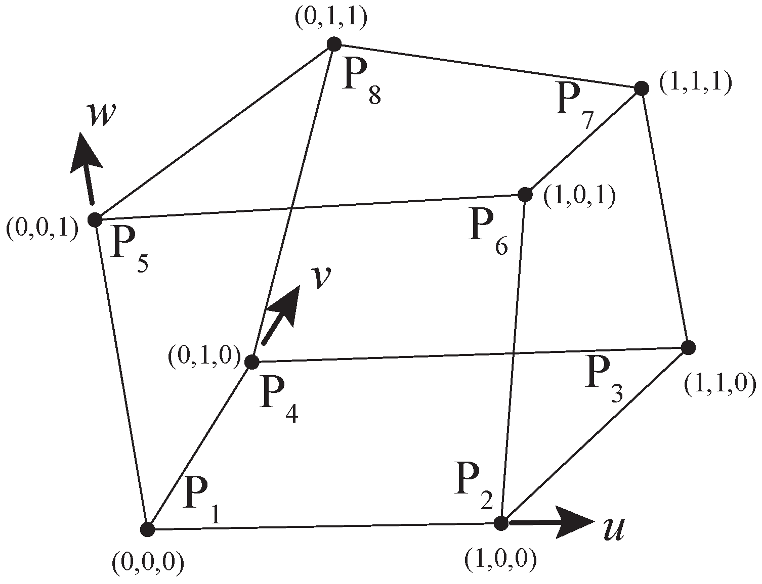
Figure 3.
(a) Interface between two 1D elements with the same material (marked element 1 and 2), (b) interface between two 1D elements with different materials.
Figure 3.
(a) Interface between two 1D elements with the same material (marked element 1 and 2), (b) interface between two 1D elements with different materials.
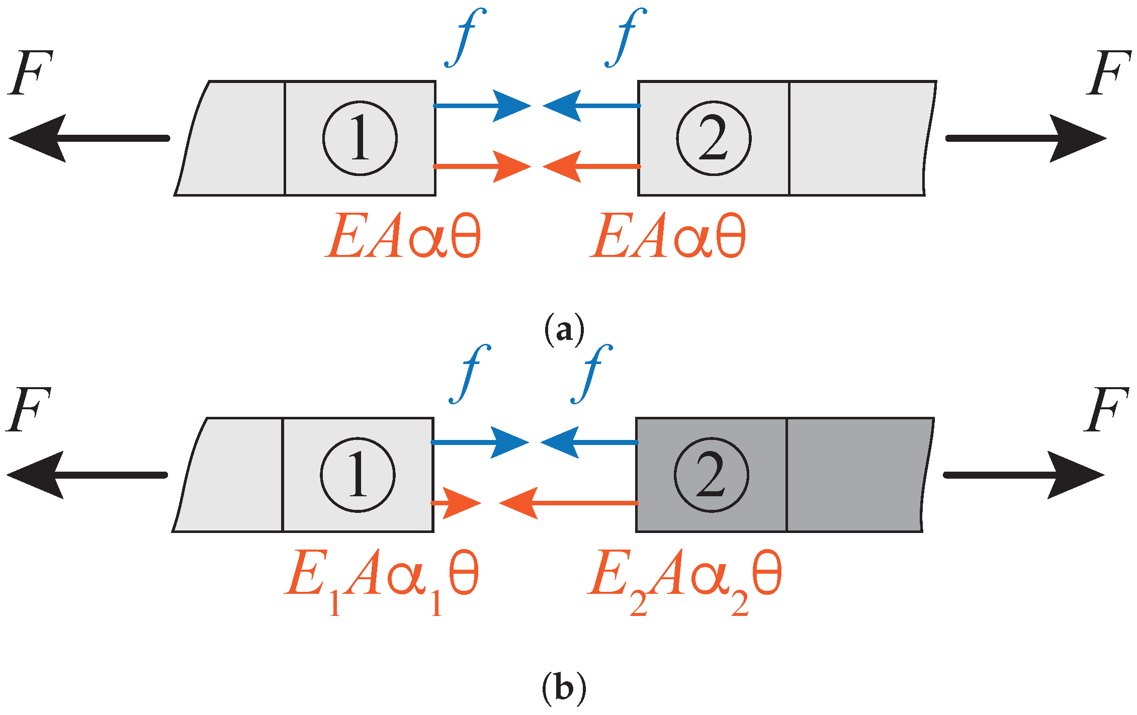
Figure 4.
Boundary identification in the linear solid hexahedral thermoelastic element.
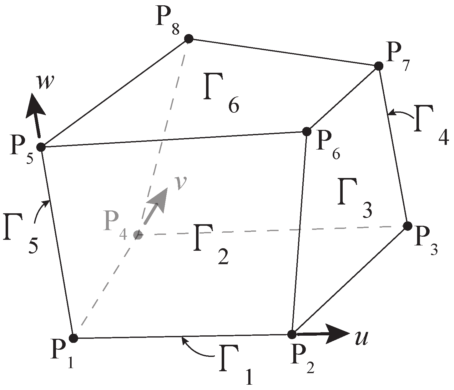
Figure 5.
(a) W150 × 100 × 24.0 wide beam flange section, (b) encased W150 beam.

Figure 6.
Beam used in the validation study, adapted from [40].
Figure 6.
Beam used in the validation study, adapted from [40].
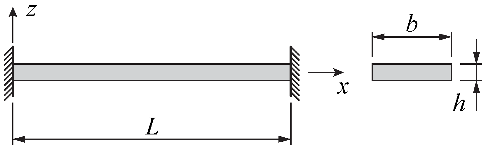
Figure 7.
Comparative study of the evolution of the quality factor () with the beam thickness (h) for the first bending mode, adapted from [40].
Figure 7.
Comparative study of the evolution of the quality factor () with the beam thickness (h) for the first bending mode, adapted from [40].
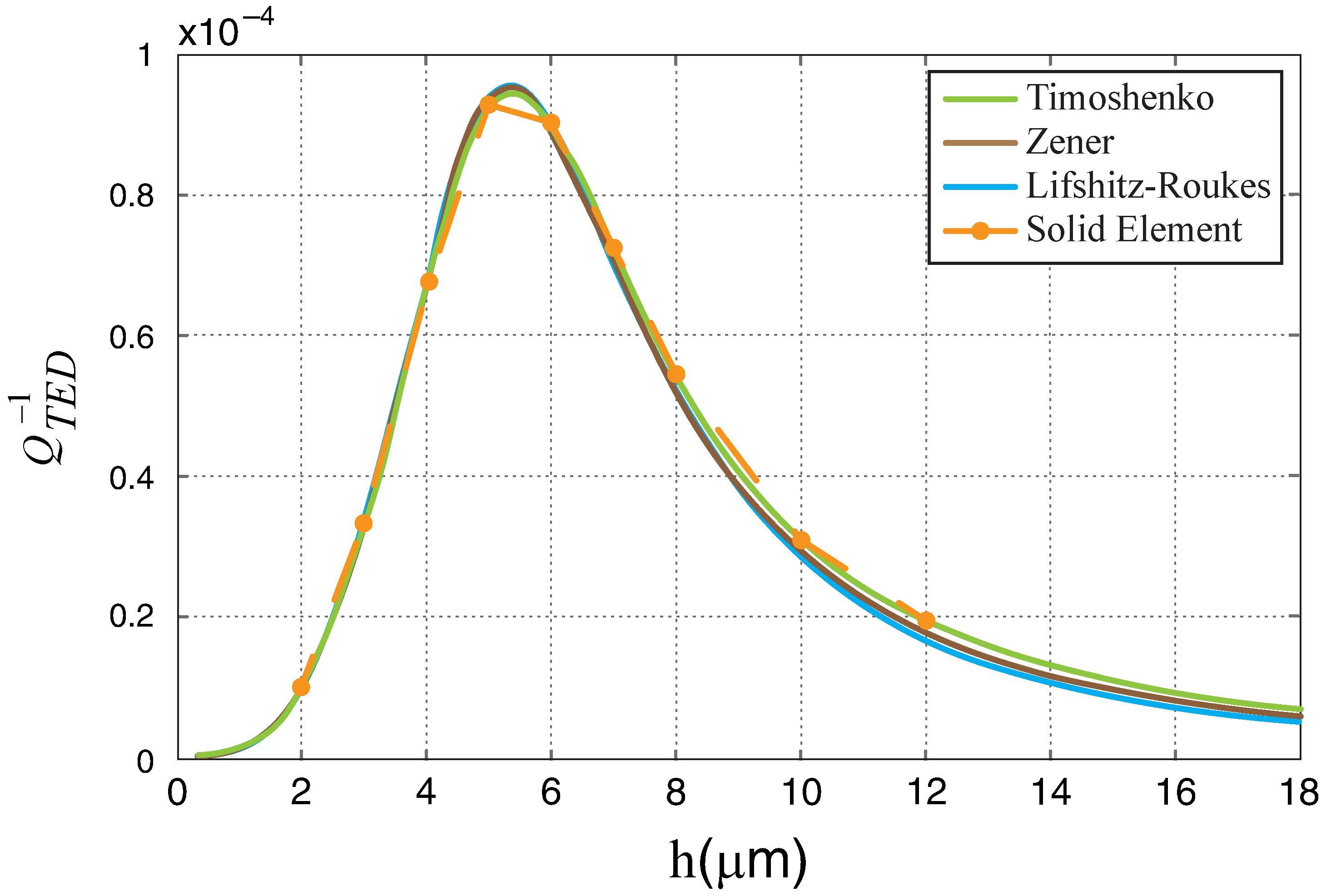
Figure 8.
(a) Convergence of the first two natural frequencies for the W150 × 100 × 24.0 beam (“•” represents the convergence of the first mode and “⋆” represents the convergence of the second mode), (b) mesh for the W150 I-beam with 240 elements across the length.
Figure 8.
(a) Convergence of the first two natural frequencies for the W150 × 100 × 24.0 beam (“•” represents the convergence of the first mode and “⋆” represents the convergence of the second mode), (b) mesh for the W150 I-beam with 240 elements across the length.

Figure 9.
(a) Convergence of the first two natural frequencies for the encased W150 × 100 × 24.0 I-beam (“•” represents the convergence of the first mode and “⋆” represents the convergence of the second mode), (b) mesh for the encased W150 I-beam with 140 elements across the length.
Figure 9.
(a) Convergence of the first two natural frequencies for the encased W150 × 100 × 24.0 I-beam (“•” represents the convergence of the first mode and “⋆” represents the convergence of the second mode), (b) mesh for the encased W150 I-beam with 140 elements across the length.
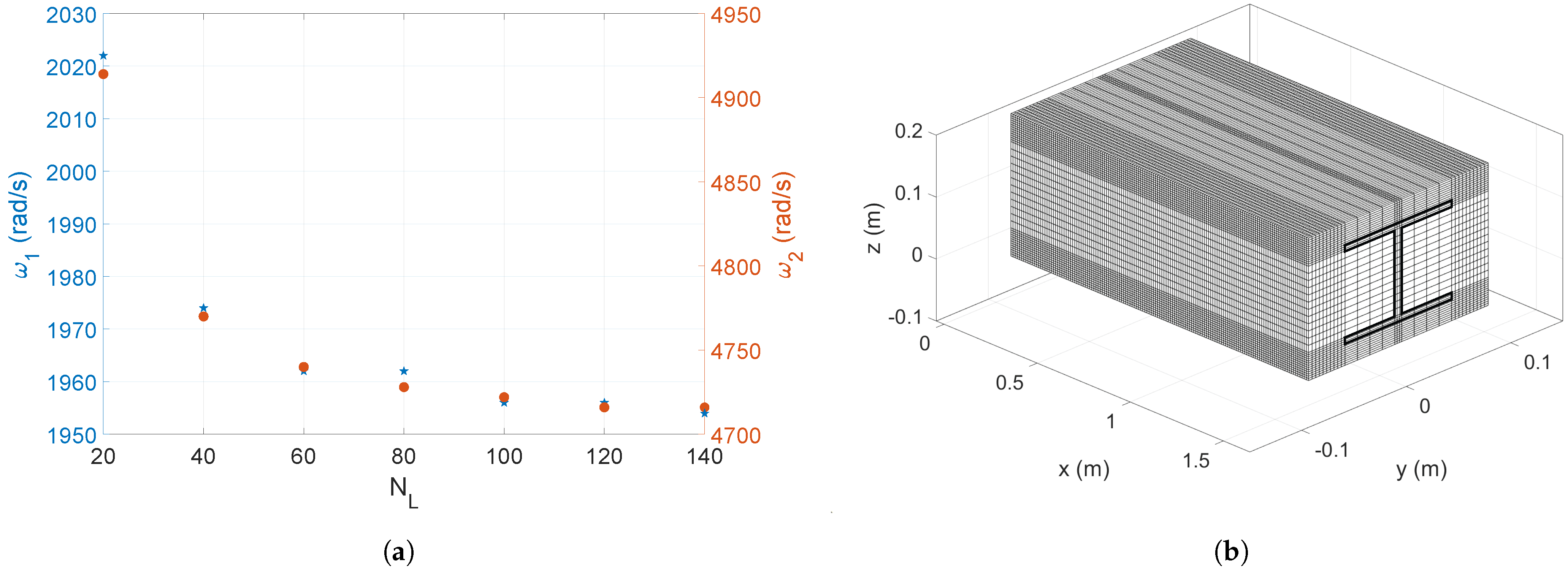
Figure 10.
Amplitude e position of the applied distributed load.
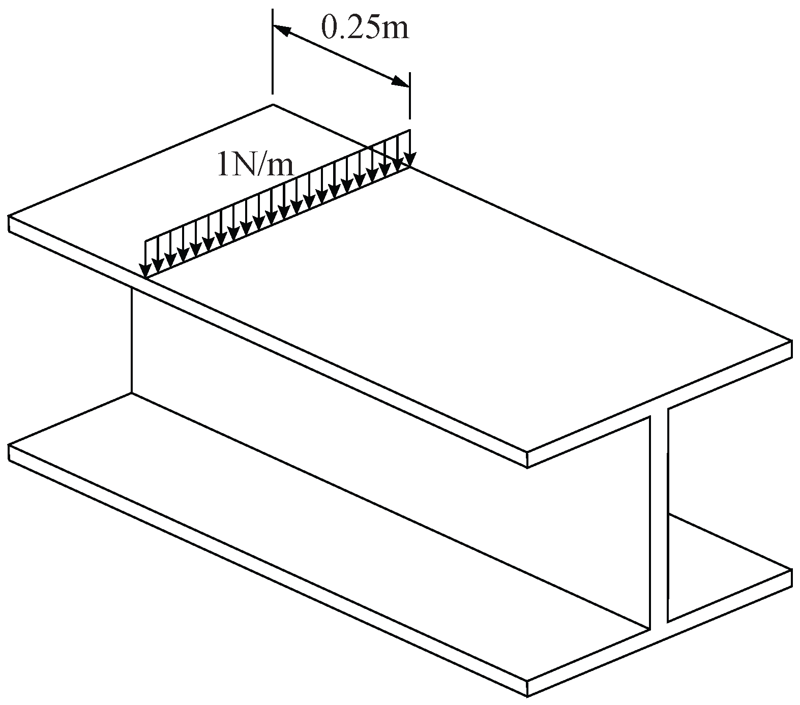
Figure 11.
Bode diagram of the long-range frequency sweep of case studies 1 to 3, measured at the center of the distributed load (point: (0.25, 0, 0.16)).
Figure 11.
Bode diagram of the long-range frequency sweep of case studies 1 to 3, measured at the center of the distributed load (point: (0.25, 0, 0.16)).
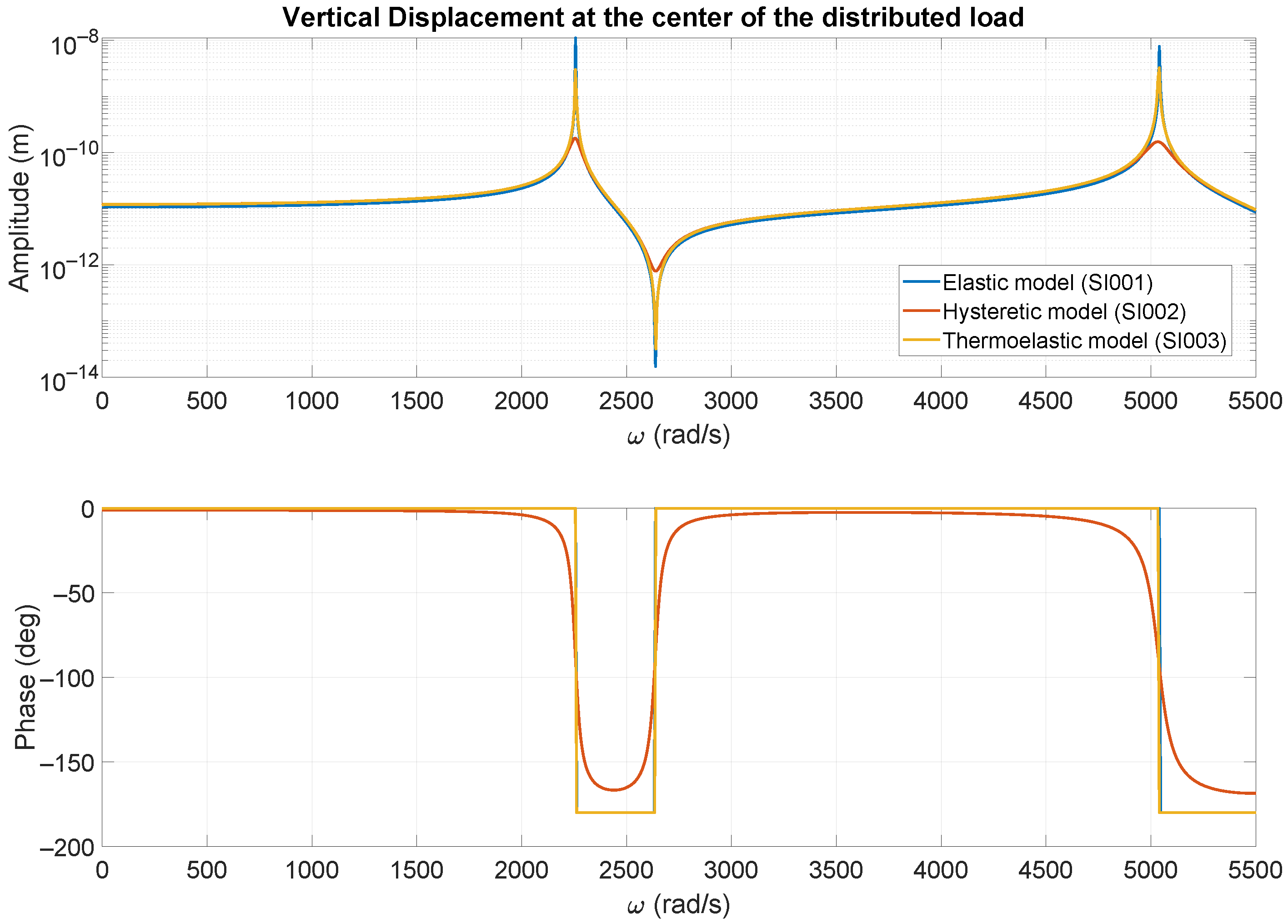
Figure 12.
(a) First mode shape of the SI003 case study, (b) mid beam cross-section showing the temperature variation across the section.
Figure 12.
(a) First mode shape of the SI003 case study, (b) mid beam cross-section showing the temperature variation across the section.
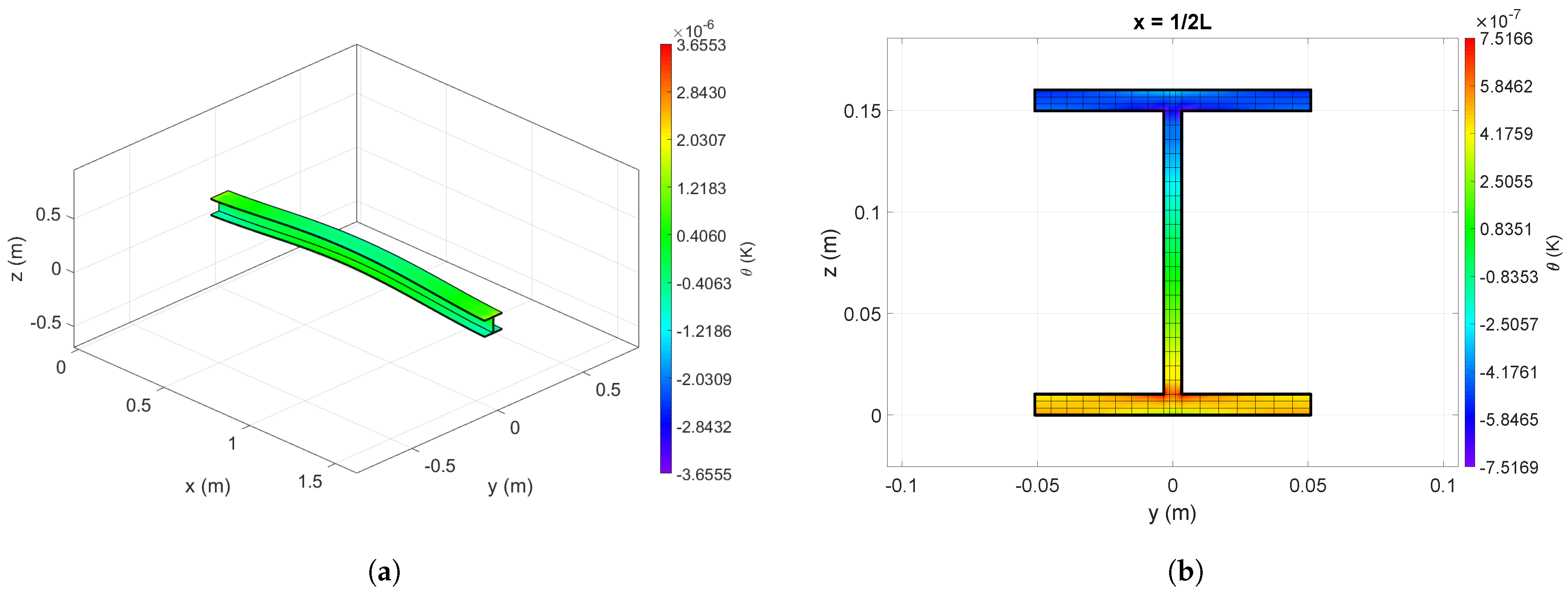
Figure 13.
Equivalent damping coefficient of case studies SI003 and SI004.
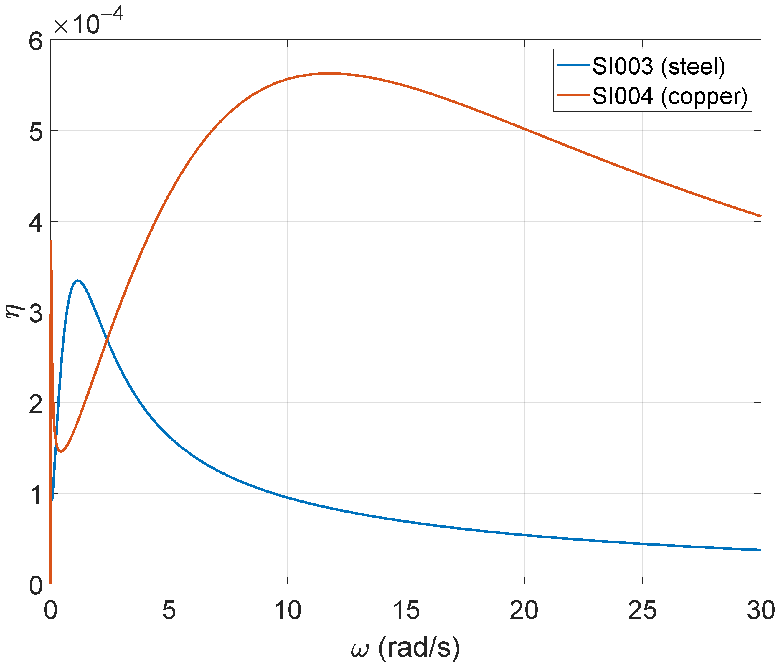
Figure 14.
Bode diagram of the long-range frequency sweep of case studies 9, 12, 18, and 19.
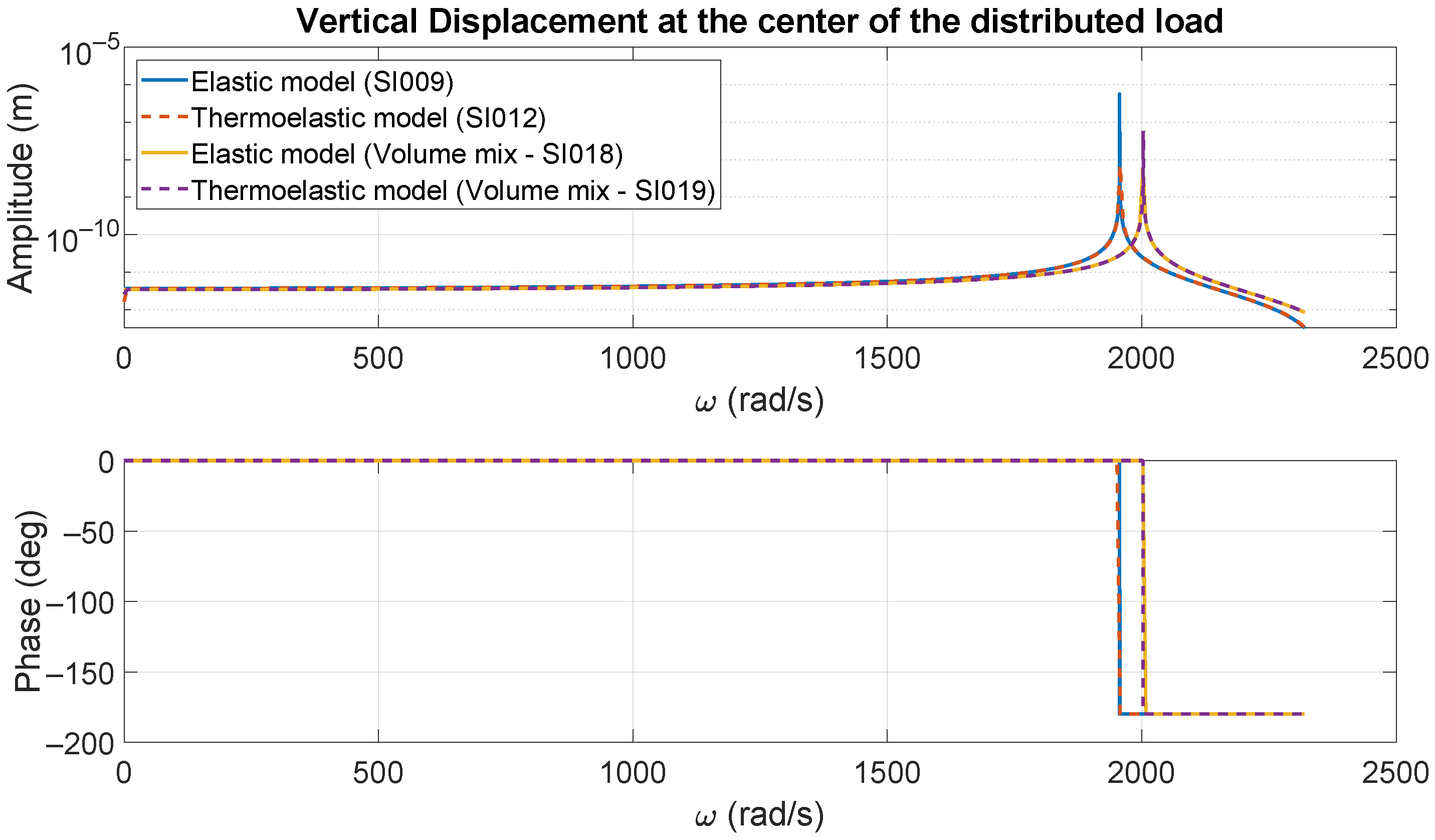
Figure 15.
(a) First mode shape of the case study SI012, (b) mid beam cross-section showing the temperature variation across the section for SI012, (c) first mode shape of the case study SI019, (d) mid beam cross-section showing the temperature variation across the section for SI019.
Figure 15.
(a) First mode shape of the case study SI012, (b) mid beam cross-section showing the temperature variation across the section for SI012, (c) first mode shape of the case study SI019, (d) mid beam cross-section showing the temperature variation across the section for SI019.
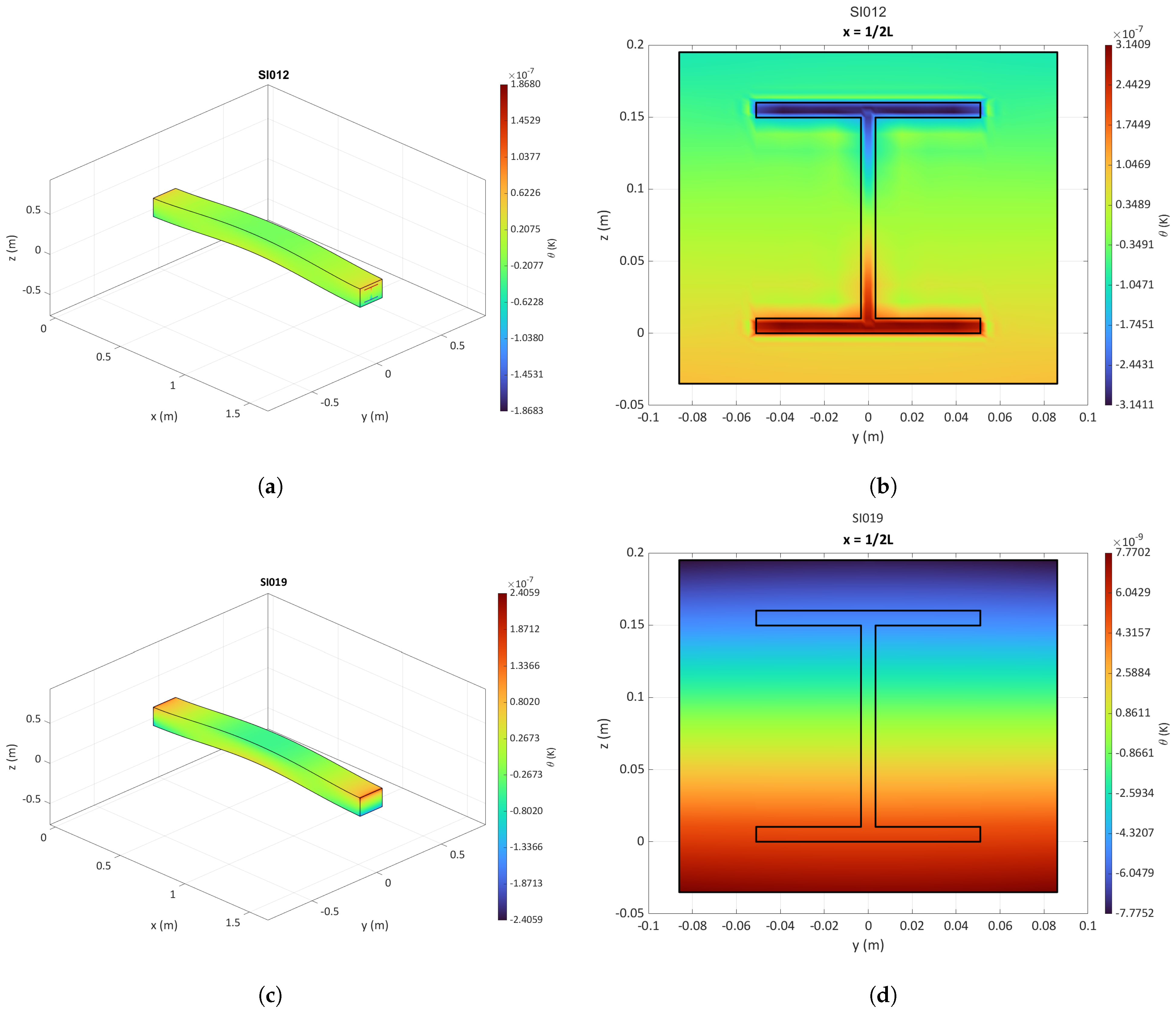
Figure 16.
Equivalent damping coefficient of case studies SI012, SI017 and SI019.
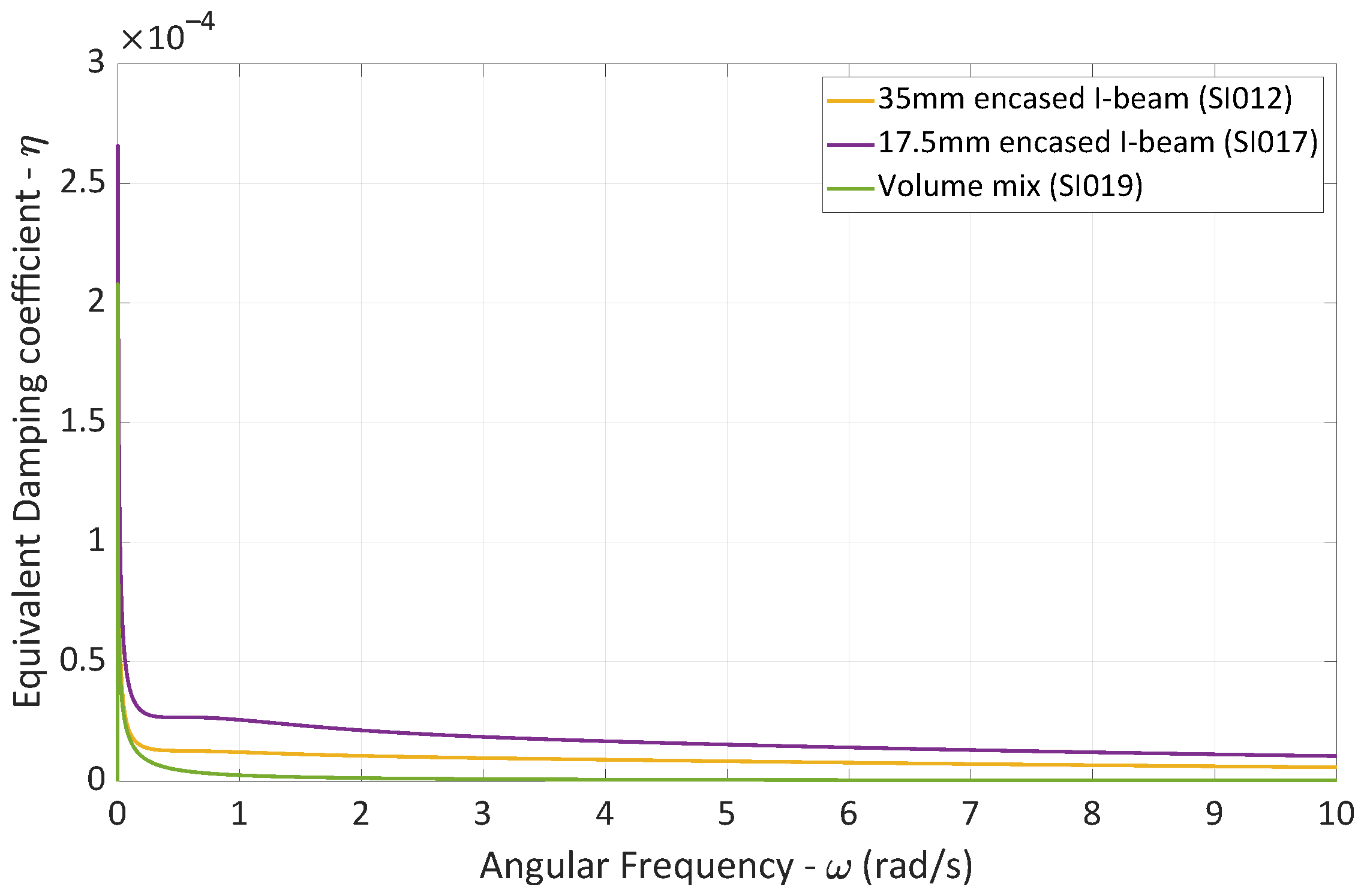
Figure 17.
Equivalent damping coefficient of case studies SI003, SI004, SI0012, SI017 and SI019.

Table 1.
Dimensions of the section of a W150 × 100 × 24.0 wide flange beam (all dimensions in mm).
| Dimension | Value |
|---|---|
| 6.6 | |
| 139.4 | |
| 102 | |
| 10.3 | |
| 102 | |
| 10.3 | |
| h | 160 |
Table 2.
Properties of the materials used in this study. All properties are taken at a base temperature, , of .
Table 2.
Properties of the materials used in this study. All properties are taken at a base temperature, , of .
| Property | Unit | Steel | Copper | Portland Cement Concrete |
|---|---|---|---|---|
| Young modulus | 200 | 120 | 34.5 | |
| Poisson coefficient | - | 0.3 | 0.355 | 0.2 |
| Density | 7800 | 8960 | 2400 | |
| Thermal expansion coefficient | ||||
| Conductivity | 45 | 401 | 0.5 | |
| Specific heat capacity | 470 | 385 | 880 |
Table 3.
Material properties of silicon [40]. All properties are taken at a base temperature, , of .
Table 3.
Material properties of silicon [40]. All properties are taken at a base temperature, , of .
| Property | Value |
|---|---|
| Young Modulus | |
| Poisson coefficient | 0.2 |
| Density | |
| Conductivity | |
| Specific heat capacity | |
| Thermal expansion coefficient |
Table 4.
Mesh convergence study for the bare W150 × 100 × 24.0 I-beam.
| No. DoF | Rel. var. | Rel. var. | |||||||||
|---|---|---|---|---|---|---|---|---|---|---|---|
| 20 | 3 | 3 | 6 | 3 | 4704 | 2376 | – | 378.15 | 5418 | – | 862.30 |
| 40 | 3 | 4 | 8 | 3 | 9184 | 2298 | 365.74 | 5172 | 823.15 | ||
| 60 | 3 | 6 | 10 | 3 | 17,568 | 2274 | 361.92 | 5106 | 812.65 | ||
| 80 | 3 | 8 | 13 | 3 | 29,808 | 2268 | 360.96 | 5076 | 807.87 | ||
| 100 | 3 | 10 | 15 | 3 | 43,632 | 2262 | 360.01 | 5058 | 805.01 | ||
| 120 | 3 | 12 | 18 | 3 | 60,016 | 2262 | 360.01 | 5046 | 803.10 | ||
| 140 | 3 | 14 | 20 | 3 | 78,960 | 2256 | 359.05 | 5040 | 802.14 | ||
| 160 | 3 | 16 | 23 | 3 | 103,040 | 2256 | 359.05 | 5034 | 801.19 | ||
| 180 | 3 | 18 | 25 | 3 | 127,424 | 2256 | 359.05 | 5034 | 801.19 | ||
| 200 | 3 | 20 | 28 | 3 | 154,368 | 2256 | 359.05 | 5028 | 800.23 | ||
| 220 | 3 | 22 | 31 | 3 | 190,944 | 2256 | 359.05 | 5028 | 800.23 | ||
| 240 | 3 | 24 | 33 | 3 | 219,792 | 2256 | 359.05 | 5028 | 800.23 |
Table 5.
Mesh convergence study for the encased W150 × 100 × 24.0 I-beam.
| No. DoF | Rel. var. | Rel. var. | ||||||||||
|---|---|---|---|---|---|---|---|---|---|---|---|---|
| 20 | 3 | 3 | 6 | 3 | 10 | 65,520 | 2022 | – | 321.81 | 4914 | – | 782.09 |
| 40 | 3 | 4 | 6 | 3 | 10 | 127,920 | 1974 | 314.17 | 4770 | 759.17 | ||
| 60 | 3 | 6 | 6 | 3 | 10 | 210,816 | 1962 | 312.26 | 4740 | 754.39 | ||
| 80 | 3 | 8 | 8 | 3 | 10 | 310,068 | 1962 | 312.26 | 4728 | 752.48 | ||
| 100 | 3 | 10 | 9 | 3 | 10 | 424,200 | 1956 | 311.31 | 4722 | 751.53 | ||
| 120 | 3 | 12 | 10 | 3 | 10 | 555,148 | 1956 | 311.31 | 4716 | 750.57 | ||
| 140 | 3 | 14 | 11 | 3 | 10 | 703,872 | 1954.59 | 311.08 | 4716.15 | 750.60 |
Table 6.
Case studies used in this work.
| ID | Section | Case Thickness | Length Ratio | No. Elements | Analysis | Material | Thermal BC |
|---|---|---|---|---|---|---|---|
| SI001 | I-beam | - | 10 H | 240 | Elastic | Steel | - |
| SI002 | I-beam | - | 10 H | 240 | Hysteretic | Steel | - |
| SI003 | I-beam | - | 10 H | 240 | Thermoelastic | Steel | Adiabatic |
| SI004 | I-beam | - | 10 H | 240 | Thermoelastic | Copper | Adiabatic |
| SI009 | Encased | 10 H | 140 | Elastic | Steel/Concrete | - | |
| SI012 | Encased | 10 H | 140 | Thermoelastic | Steel/Concrete | Adiabatic | |
| SI017 | Encased | 10 H | 140 | Thermoelastic | Steel/Concrete | Adiabatic | |
| SI018 | Encased | 10 H | 140 | Elastic | Volume mix | - | |
| SI019 | Encased | 10 H | 140 | Thermoelastic | Volume mix | Adiabatic |
Table 7.
First two resonant frequencies.
| Frequency | Elastic Model | Hysteretic Model | Thermoelastic Model |
|---|---|---|---|
| First | |||
| Second |
Table 8.
Resonant frequencies of the first mode for the encased beams simulations.
| Case-Study | Frequency |
|---|---|
| Elastic Model (SI009) | 1954 |
| Thermoelastic Model (SI012) | 1957 |
| Elastic Model (Volume mix—SI018) | |
| Thermoelastic Model (Volume mix—SI019) |
Disclaimer/Publisher’s Note: The statements, opinions and data contained in all publications are solely those of the individual author(s) and contributor(s) and not of MDPI and/or the editor(s). MDPI and/or the editor(s) disclaim responsibility for any injury to people or property resulting from any ideas, methods, instructions or products referred to in the content. |
© 2023 by the author. Licensee MDPI, Basel, Switzerland. This article is an open access article distributed under the terms and conditions of the Creative Commons Attribution (CC BY) license (https://creativecommons.org/licenses/by/4.0/).
Share and Cite
MDPI and ACS Style
Carvalho, A. Study of Damping of Bare and Encased Steel I-Beams Using the Thermoelastic Model. Buildings 2023, 13, 2964. https://doi.org/10.3390/buildings13122964
AMA Style
Carvalho A. Study of Damping of Bare and Encased Steel I-Beams Using the Thermoelastic Model. Buildings. 2023; 13(12):2964. https://doi.org/10.3390/buildings13122964
Chicago/Turabian StyleCarvalho, André. 2023. "Study of Damping of Bare and Encased Steel I-Beams Using the Thermoelastic Model" Buildings 13, no. 12: 2964. https://doi.org/10.3390/buildings13122964
Note that from the first issue of 2016, this journal uses article numbers instead of page numbers. See further details here.