
Research on the Mechanical Performance of a Mountainous Long-Span Steel Truss Arch Bridge with High and Low Arch Seats

Abstract
:1. Introduction
2. Description of the Loushui River Bridge
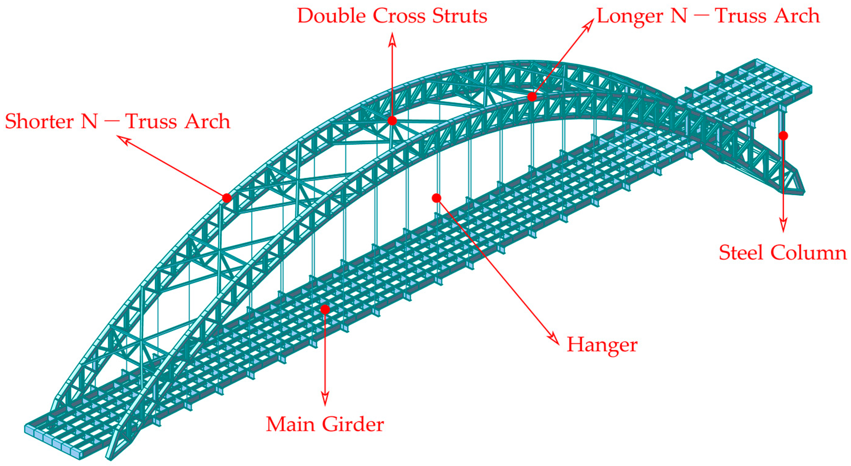
2.1. Design of the Loushui River Bridge
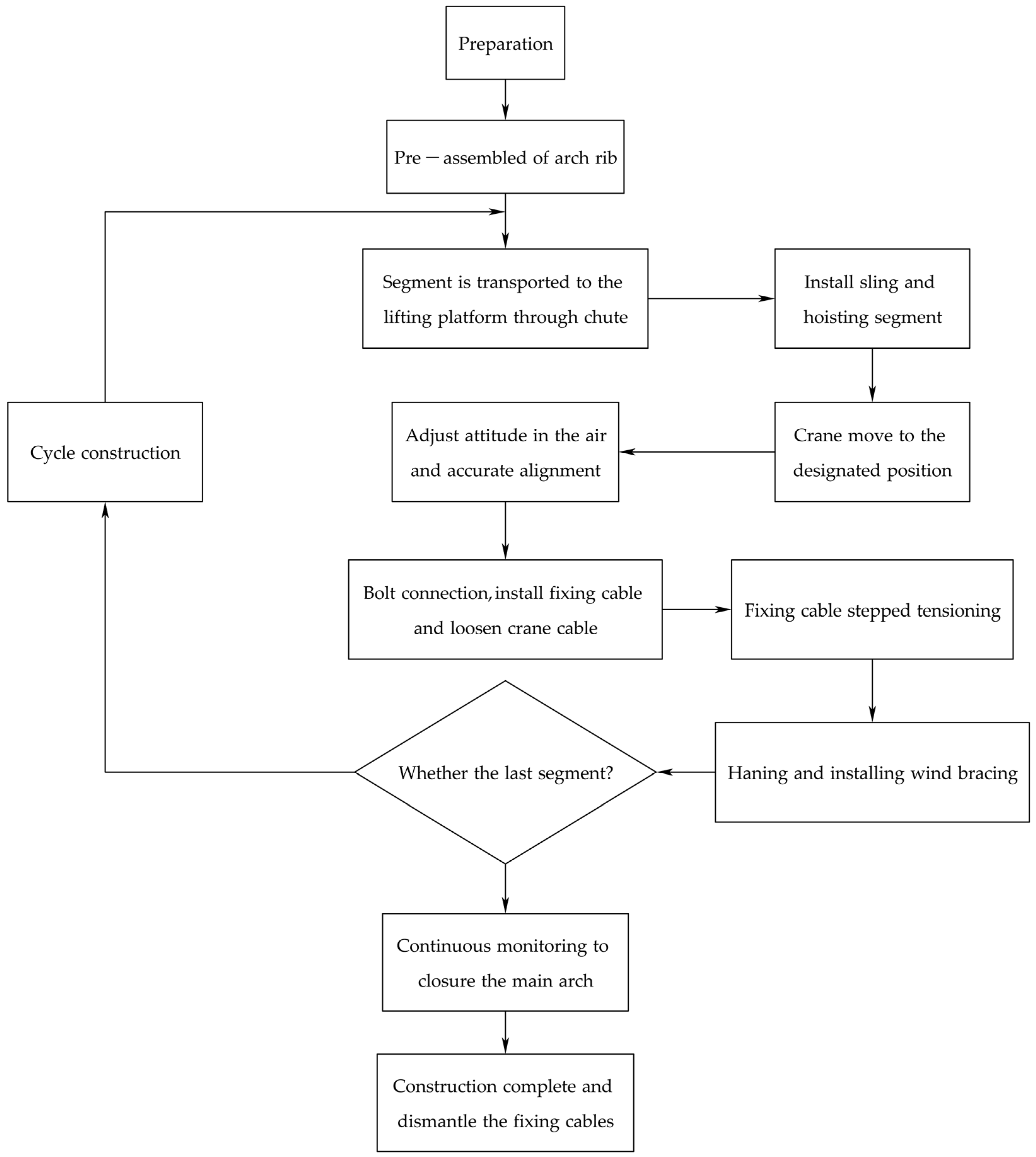
2.2. Construction of the Loushui River Bridge
3. Finite Element Simulations
4. Data Analyses from Field Experiments and Finite Element Simulations
4.1. Numerical Validation of the FE Model
4.2. Experimental Validation
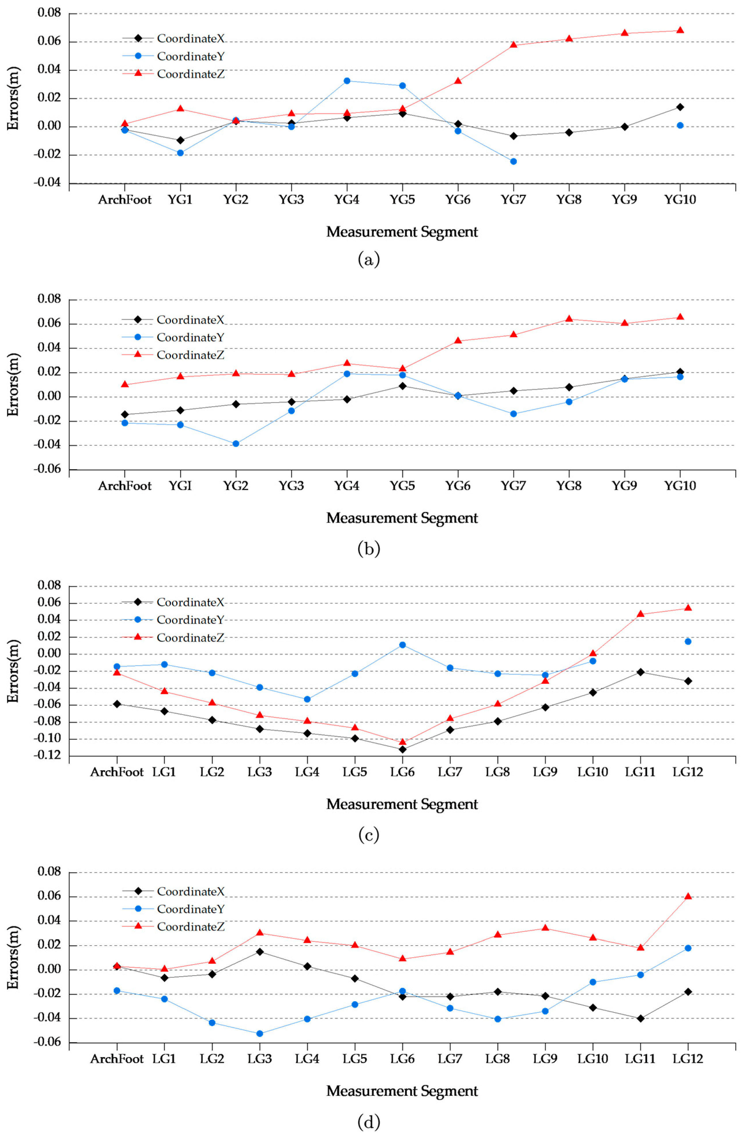
4.2.1. Validating the ANSYS Model Based on Line Control
4.2.2. Validating the ANSYS Model Based on Stress
4.3. Stability Analysis under a Wind Load
4.3.1. Buckling Analysis in the Construction Stage
4.3.2. Buckling Analysis in the Operation Stage
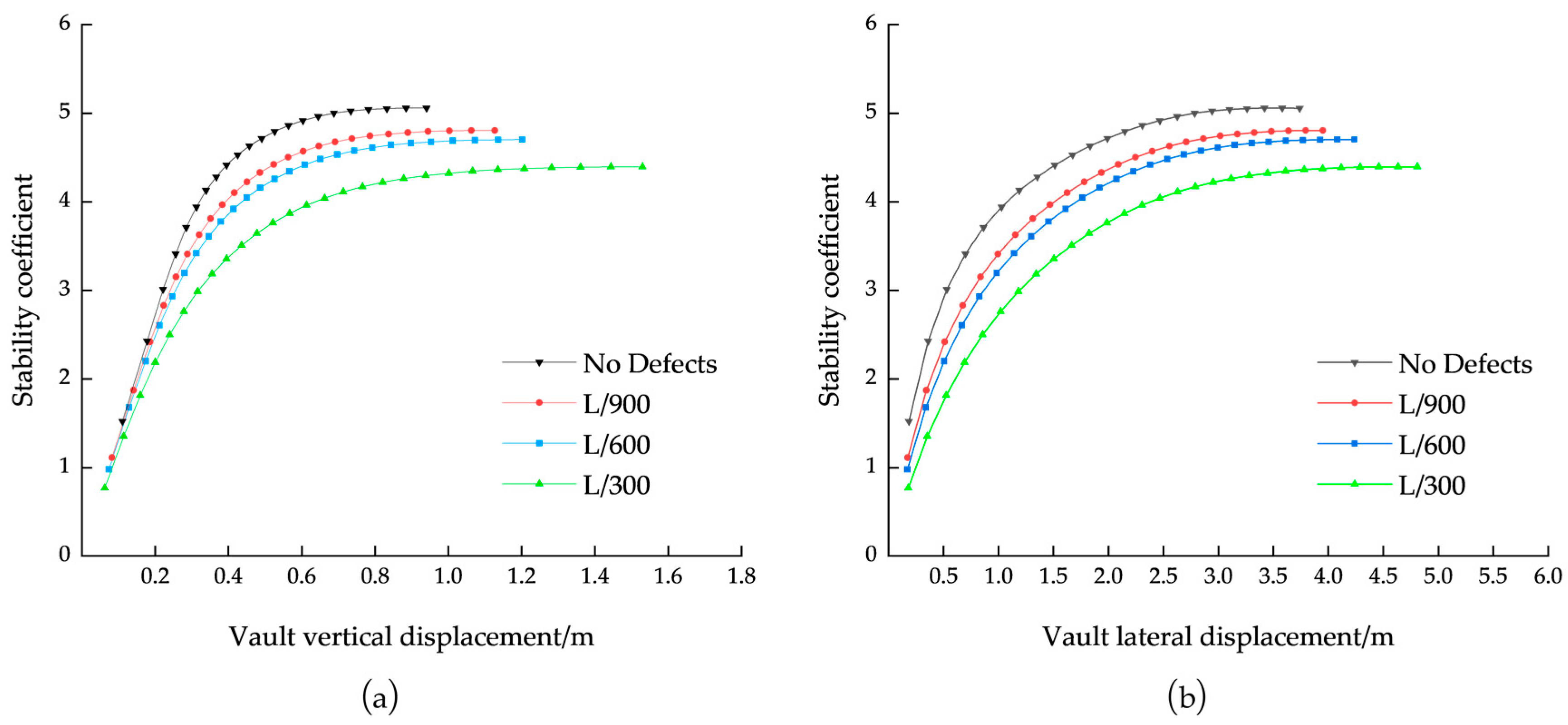
4.3.3. Stability Considering Geometric Nonlinearity
4.3.4. Stability under Material Nonlinearity
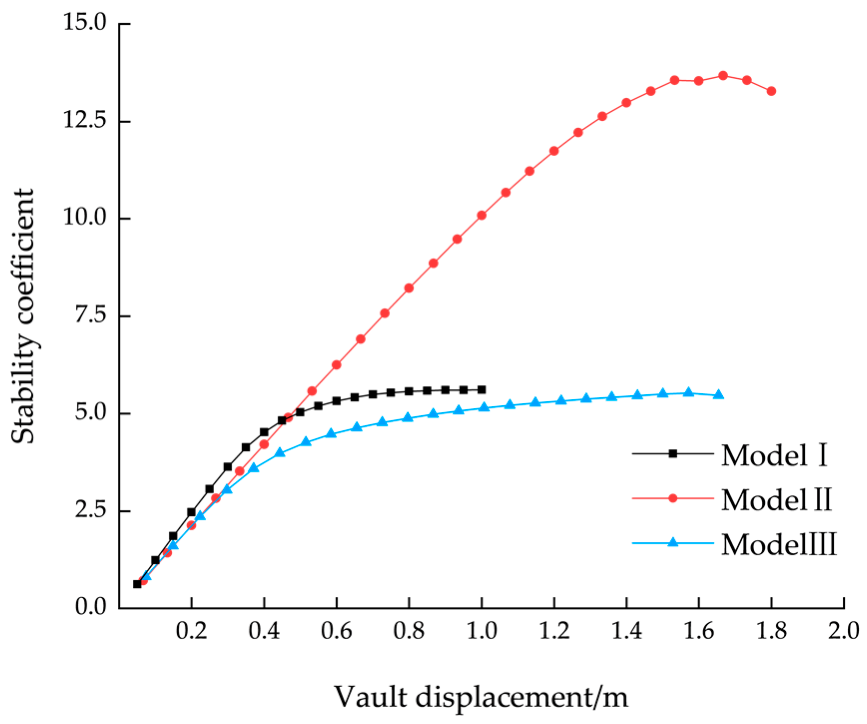
4.4. Effects of Asymmetry
4.5. Components
4.5.1. Main Components Affect Stability
4.5.2. Effects of Different Stiffnesses in Arch Ribs
4.5.3. Effects of Different Stiffnesses in Struts
4.6. Struts
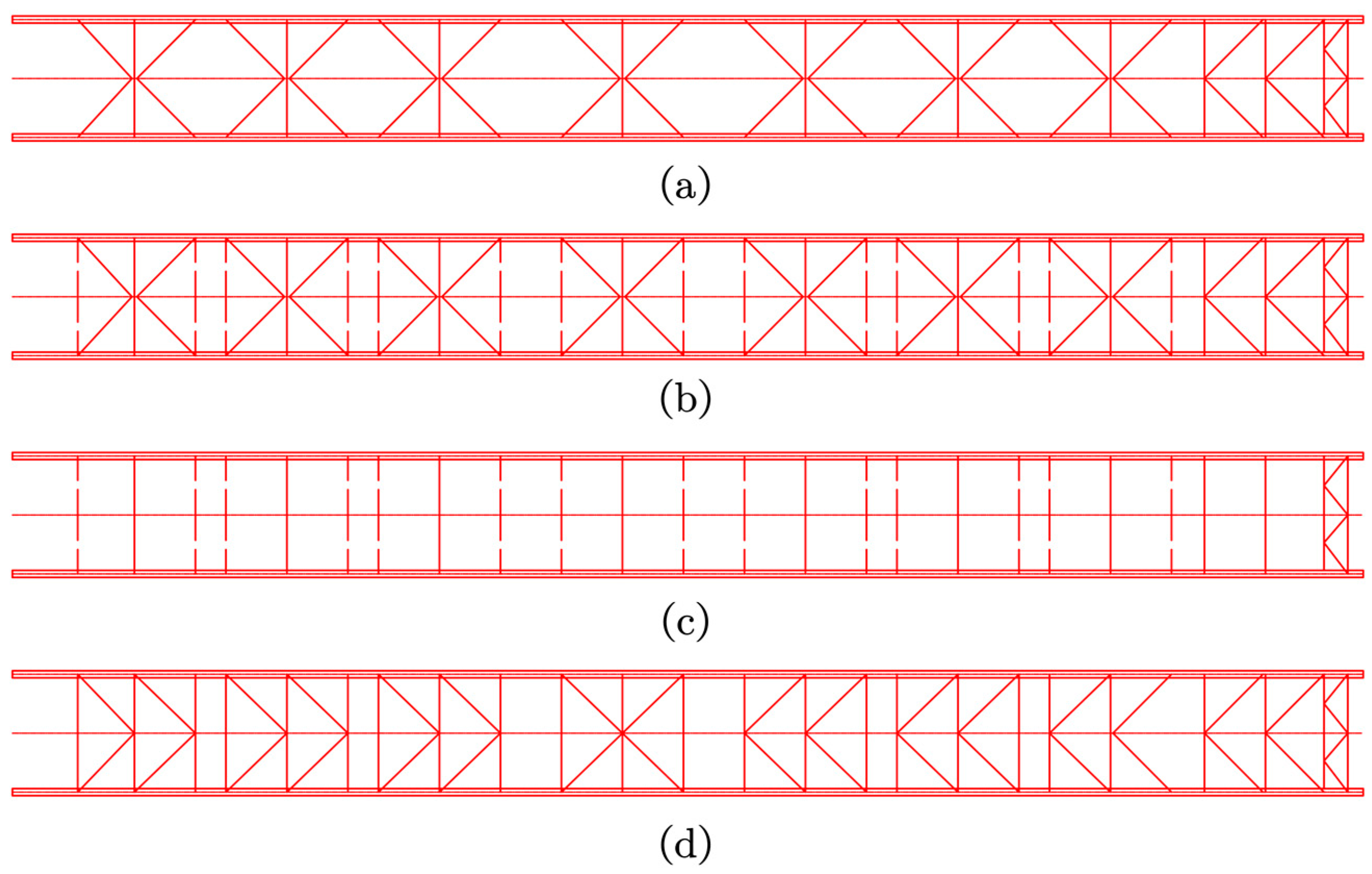
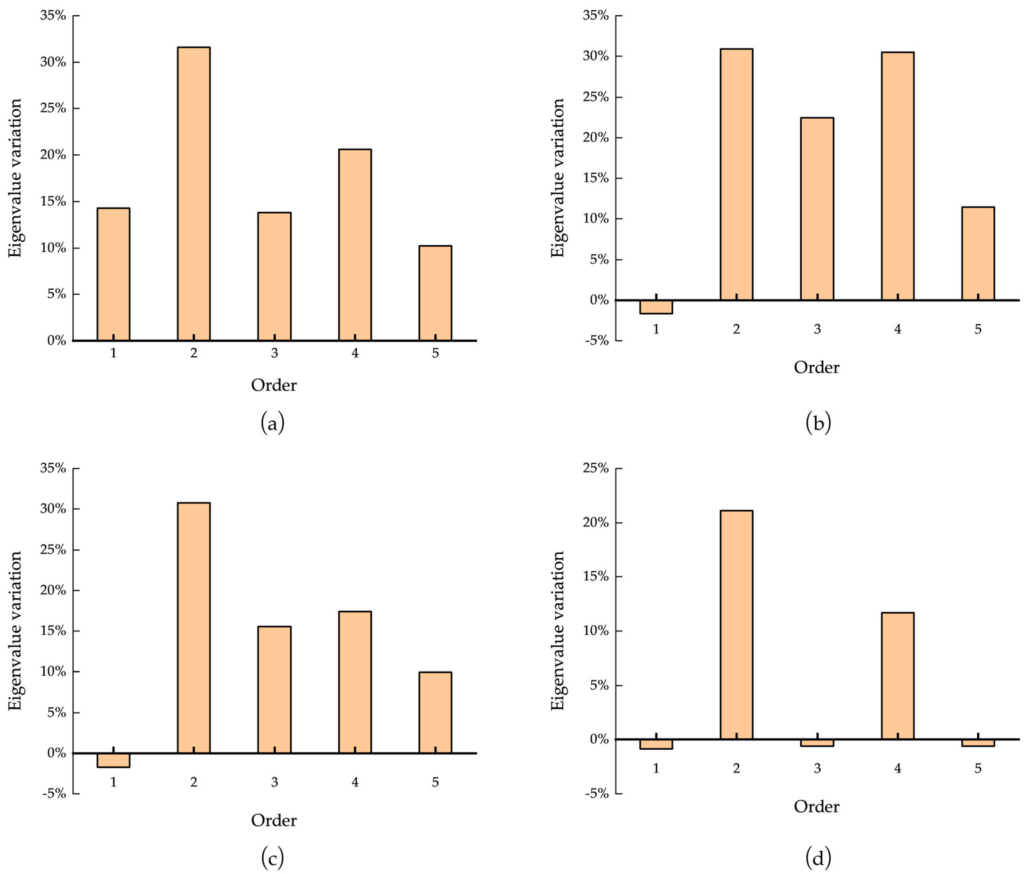
4.6.1. Stability of Different Types of Struts
- a.
- Original design: double cross struts with partial K-shaped struts;
- b.
- Doubled cross bracing at the upper and lower chords based on Scheme a;
- c.
- Removed upper and lower chord diagonal struts based on Scheme b;
- d.
- Replaced double cross struts with K-shaped braces based on Scheme b.
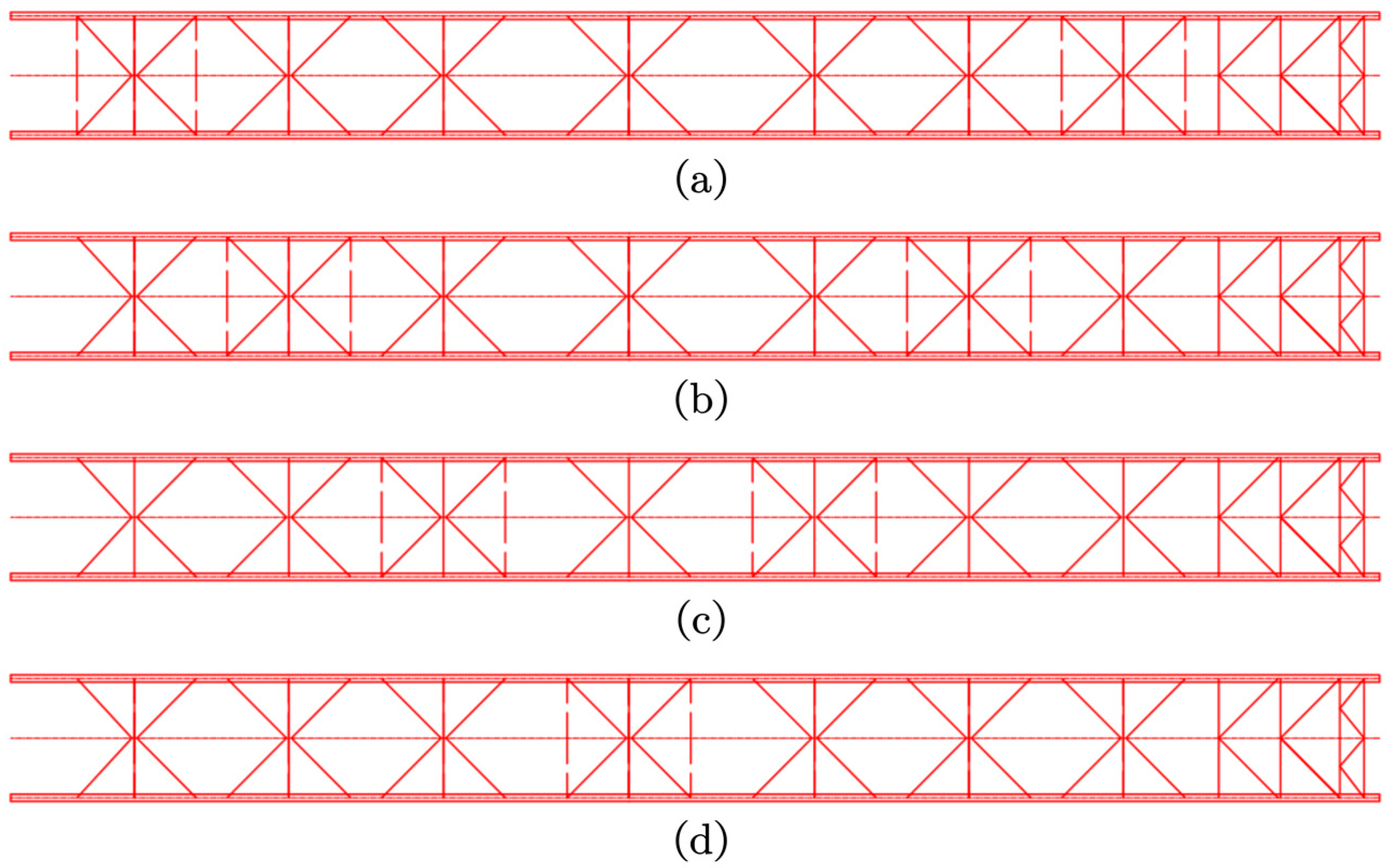
4.6.2. Stability for Adding Bracing in Certain Locations
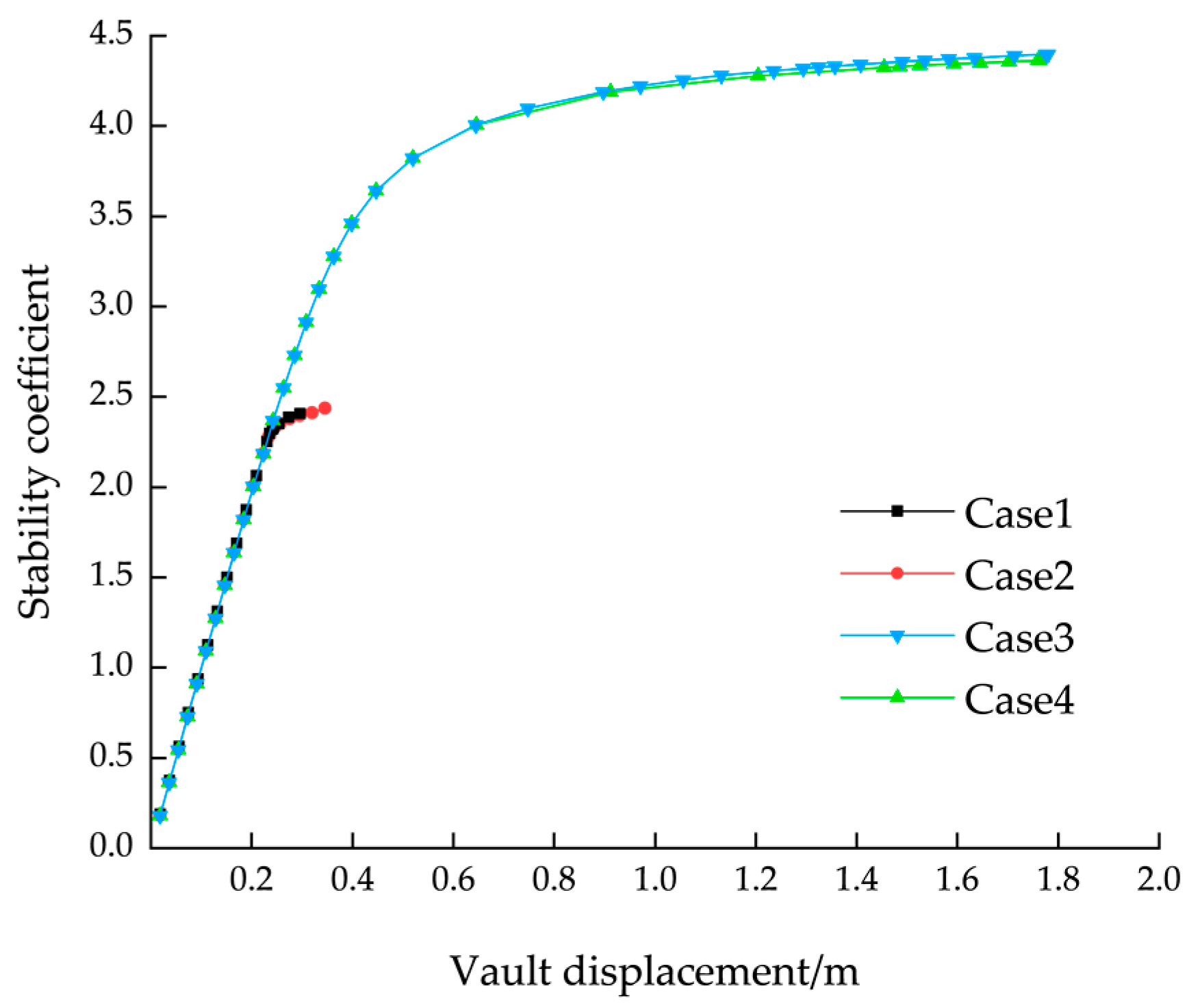
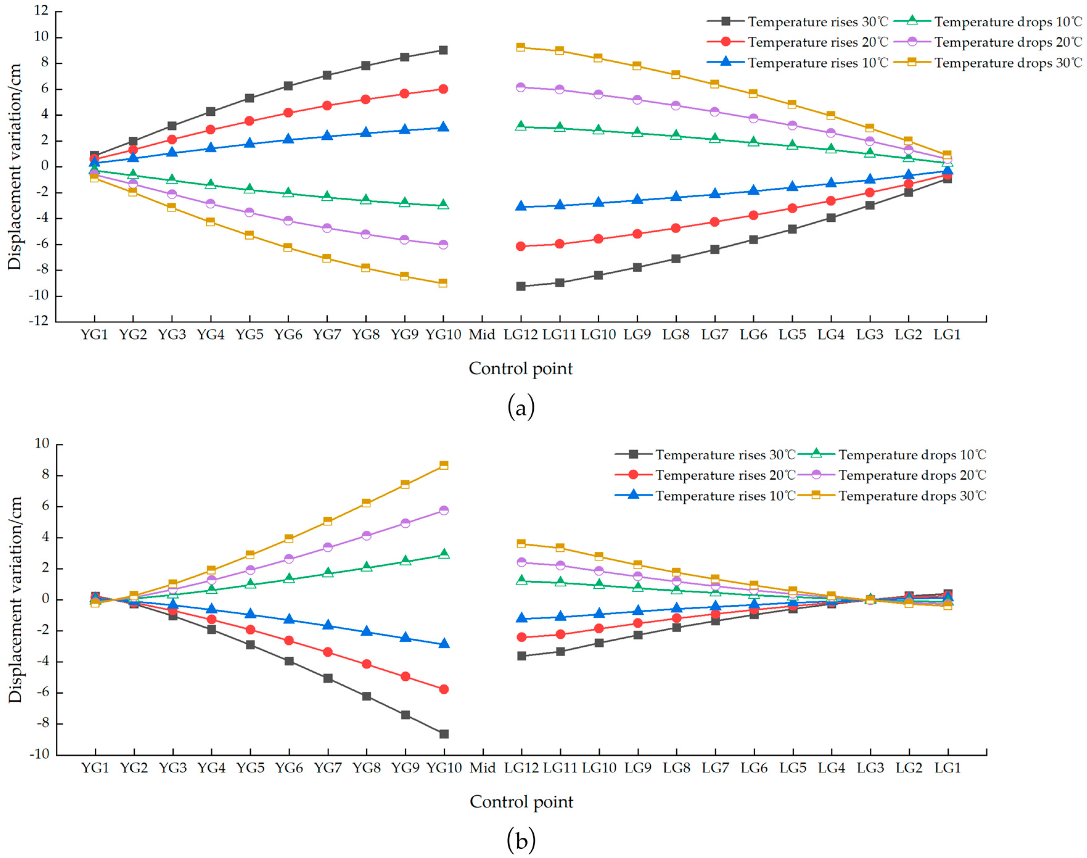
4.7. Effects of Temperature
4.7.1. Effects of Temperature under Construction
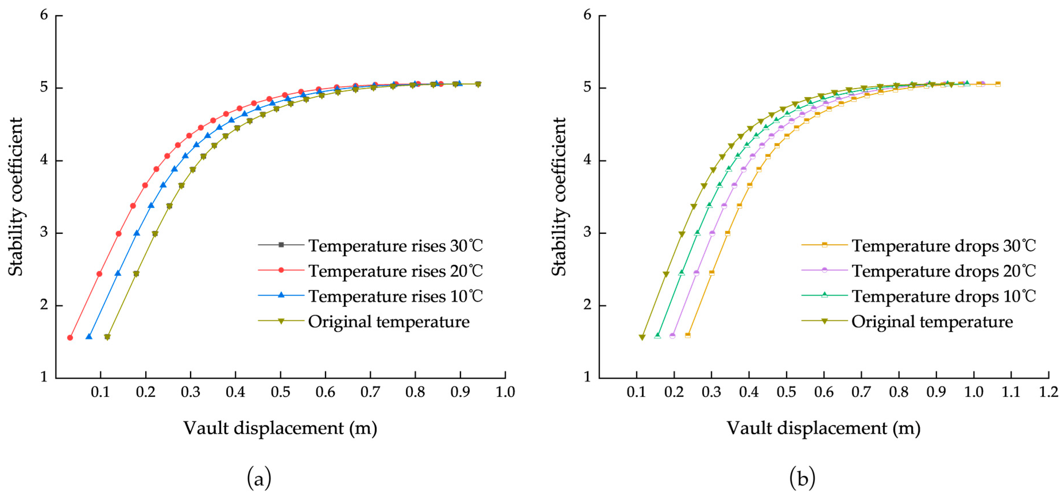
4.7.2. Effects of Temperature under Operation
5. Conclusions
- The stability of the asymmetric structure meets the design requirements in both the construction and operation stages. However, according to the buckling analysis, the dominant instability shape is out of plane, and in-plane buckling only occurs in a high order, which reflects that the bridge is most affected by lateral wind during either the construction or operation stages. Due to the influence of deep valley topography, mountain bridges should emphasize wind resistance.
- The arch rib before closure is a cantilever system, and the wind hazard in the ravine area has the greatest influence on the construction of the bridge. Compared with the windless condition, the stability of the bridge under a wind load is reduced by nearly 50%. The application of wind cables and temporary wind braces in every segment can resist the wind load well, which controls the lateral deformation of the arch rib within 5 cm.
- The geometric imperfections have a slight influence on the linear analysis of the structure, while the stability analysis when considering nonlinearity is significantly affected by imperfections. The pattern of variation shows that the bridge’s stability decreases with an increase in geometric imperfections.
- The asymmetry of the steel truss arch ribs has a significant impact on the overall stability of the bridge. Asymmetry greatly reduces the deformation tolerance of arch bridges, causing premature failure of the structures.
- The performance of steel arch ribs determines the stability of the entire arch bridge. Changes in the stiffness of the arch ribs have a greater effect on the stability, while changes in the stiffness of the wind braces have an average effect. The wind resistance of diagonal bracing is greater than that of simple transverse bracing, which can significantly improve the mechanical properties of the bridge. The weak point of the Loushui River Bridge is located at the intersection of the arch ribs and the bridge deck, where the addition of wind bracing is an effective way to improve the lateral stability and stiffness of the bridge.
- Temperature has a certain influence on the construction of arch ribs. The temperature load influence should be considered during construction, and the installation elevation of the arch rib structure should be corrected to minimize error. The effect of temperature on the stability of asymmetric steel truss arch bridges during the operational phase is not significant, and the overall stability is good, based on the environment of the Loushui River Bridge.
Author Contributions
Funding
Data Availability Statement
Conflicts of Interest
Nomenclature
| Elastic modulus | |
| Weight per unit volume of material | |
| Poisson’s ratio | |
| Yield stress of material | |
| Stress under load | |
| Total strain | |
| Elastic strain of the structure under load | |
| No-stress strain | |
| Actual elevation of the measuring point | |
| Ideal elevation of the measuring point | |
| Correction value of temperature’s influence on the structure |
References
- Zhao, W.; Xie, Q. Selection of Positions for Yesan River Bridge Foundations in Yichang-Wanzhou Railway. J. Southwest Jiaotong Univ. 2003, 16, 57–59. [Google Scholar]
- Yan, A.; Xia, Z.; Zhang, J.; Li, Z.; Yin, P. Type Selection for Youshui River Bridge of Zhangjiajie-Jishou-Huaihua Railway in Furong Town. Bridge Constr. 2021, 51, 112–117. [Google Scholar]
- Xu, Y.; Chen, D.; Nie, Z. Erection Techniques for Arch Ring of Long-Span Steel Box Truss Arch Bridge. World Bridges 2020, 48, 35–39. [Google Scholar]
- Wang, R. Key Construction Techniques for Long-Span Railway Arch Bridge in Mountainous Region of Plateau. Bridge Constr. 2020, 50, 105–110. [Google Scholar]
- Jianpeng, S.; Jinbin, L.; Yingbiao, J.; Xiaogang, M.; Zihan, T.; Zhufu, G. Key Construction Technology and Monitoring of Long-Span Steel Box Tied Arch Bridge. Int. J. Steel Struct. 2023, 23, 191–207. [Google Scholar] [CrossRef]
- Liu, Z. Arch Rib Erection Techniques of Long-Span Asymmetric Arch Bridge in Mountainous Area. World Bridges 2023, 51, 39–46. [Google Scholar] [CrossRef]
- Wang, Y. Construction Techniques for Erection of Arch Rib of Main Bridge of Guizhou Yachi River Bridge on Chengdu-Guiyang Railway. Bridge Constr. 2017, 47, 104–108. [Google Scholar]
- Fang, N.; Xu, X.; Wang, S. Design of Heavy Cable Crane for Zigui Changjiang River Highway Bridge. Bridge Constr. 2022, 52, 116–123. [Google Scholar]
- Hui-Jun, L.; Zeng-Li, P.; Chun-Liang, Y.; Yue-Ming, T. Application of Advanced Reliability Algorithms in Truss Structures. Int. J. Space Struct. 2014, 29, 61–70. [Google Scholar] [CrossRef]
- Bonopera, M.; Chang, K.-C.; Chen, C.-C.; Lin, T.-K.; Tullini, N. Bending tests for the structural safety assessment of space truss members. Int. J. Space Struct. 2018, 33, 138–149. [Google Scholar] [CrossRef]
- Maes, K.; Peeters, J.; Reynders, E.; Lombaert, G.; De Roeck, G. Identification of axial forces in beam members by local vibration measurements. J. Sound Vib. 2013, 332, 5417–5432. [Google Scholar] [CrossRef]
- Wang, Y.; Ibarra, L.; Pantelides, C. Seismic Retrofit of a Three-Span RC Bridge with Buckling-Restrained Braces. J. Bridge Eng. 2016, 21, 04016073. [Google Scholar] [CrossRef]
- Celik, O.C.; Bruneau, M. Seismic behavior of bidirectional-resistant ductile end diaphragms with buckling restrained braces in straight steel bridges. Eng. Struct. 2009, 31, 380–393. [Google Scholar] [CrossRef]
- Wang, J.; Ma, P. Mechanical performance analysis of long-span steel truss arch bridge during construction process. Highw. Eng. 2022, 67, 204–209. [Google Scholar]
- Chai, S.B.; Yang, Q.H.; Wang, X.L.; Yu, Y.L.; Zhuang, H.F. Stability Analysis of Long-span Half-through Steel Box Tied Arch Bridge during Construction. Sci. Technol. Eng. 2022, 22, 8095–8102. [Google Scholar]
- Tong, X.L.; Fang, Z. Study on Stability Safety Factor of Bridge Structure Based upon Reliability Index. J. China Railw. Soc. 2014, 36, 102–108. [Google Scholar]
- Dou, C.; Jiang, Z.Q.; Pi, Y.L.; Gao, W. Elastic buckling of steel arches with discrete lateral braces. Eng. Struct. 2018, 156, 12–20. [Google Scholar] [CrossRef]
- Zhao, M.; Chen, S.T.; Sun, Z.X.; Xu, H.W.; Huang, X.M. Study on Stability of New Long-span Railway Emergency Steel Truss Girder. J. China Railw. Soc. 2022, 44, 119–127. [Google Scholar]
- Sun, X.P.; Zheng, B.; Hu, J. Analysis Method of the Second Order Aerostatic Stability for Long-span Steel Truss Arch Bridge. Highw. Eng. 2017, 42, 337–342. [Google Scholar]
- Lyu, L.; Zhong, H.; Gu, Y.; Ren, W.; Zhao, L. Main Arch Ring Nonlinear Stability Assessment of Nanpan River Super Large Bridge on Yunnan-Guangxi Railway. Railw. Eng. 2019, 59, 27–31. [Google Scholar]
- Bouras, Y.; Vrcelj, Z. Non-linear in-plane buckling of shallow concrete arches subjected to combined mechanical and thermal loading. Eng. Struct. 2017, 152, 413–423. [Google Scholar] [CrossRef]
- Yan, Q.; Luo, N.; Han, D.; Wang, W. Nonlinearity and Stability Analysis for A Long-Span Arch Bridge. J. South China Univ. Technol. 2000, 13, 64–68. [Google Scholar]
- Han, X.; Zhu, B.; Zhang, L.; Zhu, J.B.; Xiang, B.S. Dual Non-Linear Stability Research on Long-Span Concrete-Filled Steel Tubular Arch Bridge. J. Chongqing Jiaotong Univ. 2013, 32, 856–859. [Google Scholar]
- Shi, Z.; Zhang, Y.; Zhang, Y.Z.; Xia, Z.C. Study on Stability of Long-Span Railway Through Bridge with Steel Truss Girder and Flexible Arch. China Railw. Sci. 2019, 40, 52–58. [Google Scholar]
- Chen, J.; Hu, W.J. Study on Overall Stability of Long-span Deck Concrete-filled Steel Tubular Arch Bridge. Railw. Eng. 2020, 60, 16–19. [Google Scholar]
- Zhang, J.Q.; Ji, R.C. Elastic Stability Analysis of Railway Long Span CFST Arch Bridge. Railw. Eng. 2020, 60, 12–15. [Google Scholar]
- Kong, D.D.; Yu, X.K.; Hao, X.W.; Yu, Y.; Gu, Z.F. Influence of Local Instability of Members on Overall Stability of Steel Truss Arch Bridge. J. Northeast For. Univ. 2021, 49, 116–121. [Google Scholar] [CrossRef]
- Wei, Y.; Jin, Z. Research on Wind Resistance of Stiff-Skeleton Arch Ring of Long-Span Concrete-Filled Steel Tubular Arch Bridge During Vertical Rotation Construction. Bridge Constr. 2023, 53, 75–81. [Google Scholar] [CrossRef]
- Su, Y.-H.; Wu, Y.-R.; Sun, Q. Wind-Induced Response Analysis for a Fatigue-Prone Asymmetric Steel Arch Bridge with Inclined Arch Ribs. Adv. Mater. Sci. Eng. 2022, 2022, 3489390. [Google Scholar] [CrossRef]
- Li, X.; Yan, M.; Luo, P.; Yu, Q. Study on Mechanical Characteristics of Asymmetric Curved Arch Bridge with Outward-Inclined Ribs. Railw. Stand. Des. 2014, 58, 81–84. [Google Scholar] [CrossRef]
- Hu, X.K.; Xie, X.; Tang, Z.Z.; Shen, Y.G.; Wu, P.; Song, L.F. Case study on stability performance of asymmetric steel arch bridge with inclined arch ribs. Steel Compos. Struct. 2015, 18, 273–288. [Google Scholar] [CrossRef]
- Hu, X.; Huang, Y.; Wang, D.; Liu, A. Numerical simulation study of a long-span asymmetric bowstring arch bridge. Highway 2021, 66, 208–213. [Google Scholar]
- Sun, J.; Xie, J.; Liu, C. Investigating asymmetric spatial butterfly-shaped steel arch bridges: A case study. Proc. Inst. Civ. Eng.-Bridge Eng. 2021, 174, 13–27. [Google Scholar] [CrossRef]
- Peng, G.; Gao, W.; Wu, Q. Parameter analysis on the stability of butterfly shape arch bridge. J. Fuzhou Univ. 2017, 45, 512–516. [Google Scholar]
- Cheng, X.X.; Dong, J.; Cao, S.S.; Han, X.L.; Miao, C.Q. Static and Dynamic Structural Performances of a Special-Shaped Concrete-Filled Steel Tubular Arch Bridge in Extreme Events Using a Validated Computational Model. Arab. J. Sci. Eng. 2018, 43, 1839–1863. [Google Scholar] [CrossRef]
- Ma, M.; Qian, Y.; Xu, B. Analysis of Ultimate Load-Carrying Capacity of Crescent-Shaped Concrete-Filled Steel Tube Arch Bridge. J. Southwest Jiaotong Univ. 2017, 52, 678–684+714. [Google Scholar]
- Li, S.Y.; Kohlmeyer, C.; Muller, F. Global Stability Analysis of an Asymmetrical Long-Span Concrete-Filled Steel Tube Arch Bridge. In Proceedings of the ARCH’10—6th International Conference on Arch Bridges, Fuzhou, China, 11–13 October 2010; p. 7. [Google Scholar]
- Gou, H.; He, Y.; Zhou, W.; Bao, Y.; Chen, G. Experimental and numerical investigations of the dynamic responses of an asymmetrical arch railway bridge. Proc. Inst. Mech. Eng. Part F J. Rail Rapid Transit 2018, 232, 2309–2323. [Google Scholar] [CrossRef]
- Liu, X.H.; Ding, D.H.; Feng, P.C. Key Design Techniques of Long-Span Two-Hinge Steel Truss Arch Bridge with High and Low Arch Seats. Bridge Constr. 2022, 52, 101–108. [Google Scholar]
- GB 50017-2003; Code for Design of Steel Structures. Standardization Administration of China: Beijing, China, 2003.
- JTG D60-2004; General Code for Design of Highway Bridges and Culverts. CCCC First Highway Construction Co., Ltd.: Beijing, China, 2004.
- GB/T 714-2015; Structural Steel for Bridge. Standardization Administration of China: Beijing, China, 2015.
- Ge, J.Y. Guide for Use of Midas Civil Bridge Engineering Software; People’s Communications Press: Beijing, China, 2013. [Google Scholar]
- JTG/T D60-01-2004; Wind-Resistant Design Specification for Highway Bridges. CCCC First Highway Construction Co., Ltd.: Beijing, China, 2004.
- ANSYS. Structural Finite Element Analysis (FEA) Software; ANSYS Inc.: Canonsburg, PA, USA, 2022. [Google Scholar]


| Structural Component | Section Type | ) | ) | ) | Torsional Moment of Inertia (m4) |
|---|---|---|---|---|---|
| Main arch | Box section | 0.28223 | 0.09695 | 0.07915 | 0.11412 |
| Webbing of main arch | I-shaped section | 0.09392 | 0.03056 | 0.00682 | 0.01414 |
| Struts | Box section | 0.06275 | 0.00332 | 0.00299 | 0.00464 |
| Webbing of main arch | I-shaped section | 0.03784 | 0.00078 | 0.00212 | 0.00001 |
| Longitudinal beam | I-shaped section | 0.05770 | 0.03254 | 0.00115 | 0.00002 |
| Crossbeam | I-shaped section | 0.07363 | 0.07016 | 0.00156 | 0.00003 |
| Steel column | Box section | 0.13024 | 0.04210 | 0.02917 | 0.04514 |
| Hanger | Circle section | 0.00581 | / | / | / |
| Material | (Mpa) | (kN/m3) | (Mpa) | ||
| Arch steel | 2.06 × 10⁵ | 86.39 | 0.3 | 260 | |
| Deck steel | 2.06 × 10⁵ | 78.50 | 0.3 | 260 | |
| Hangers | 2.05 × 10⁵ | 81.84 | 0.3 | 1770 | |
| Information | Midas Civil 2021 | ANSYS 2022 R2 | |
|---|---|---|---|
| Construction | Operation | Operation | |
| Nodes | 2858 | 1713 | 889 |
| Elements | 6981 | 2259 | 1421 |
| Mesh size of one beam | Length of every single member | ||
| FE Model Established in Midas | FE Model Established in ANSYS | |||||
|---|---|---|---|---|---|---|
| Mode No. | Modal Frequency (Hz) | Mode Shape | Mode No. | Modal Frequency (Hz) | Mode Shape | Difference (%) |
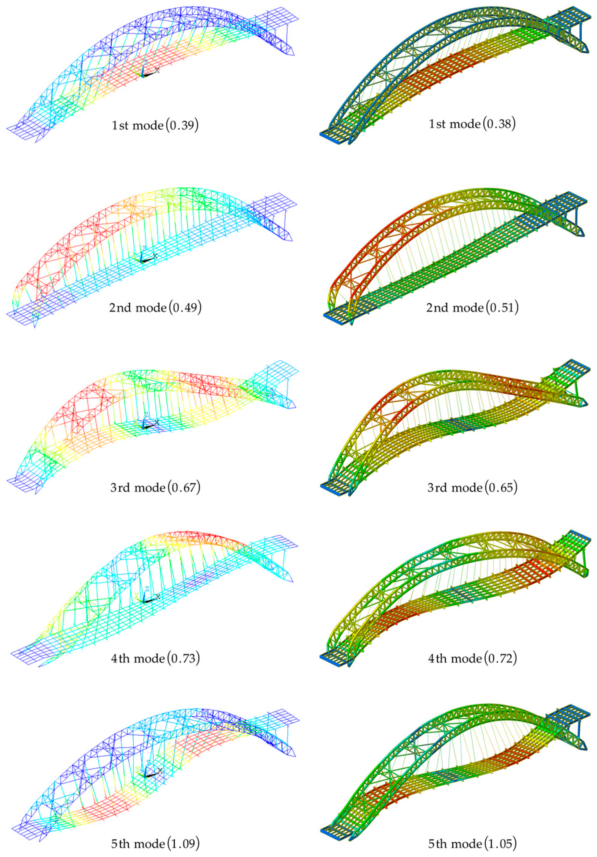
| 1 | 0.38 | Deck’s lateral bending in midspan | 1 | 0.39 | Deck’s lateral bending in midspan | −3.1 |
| 2 | 0.51 | Short side arch’s lateral bending | 2 | 0.49 | Short side arch’s lateral bending | 2.1 |
| 3 | 0.65 | Whole bridge’s asymmetry vertical bending | 3 | 0.67 | Whole bridge’s asymmetrical vertical bending | −3.5 |
| 4 | 0.72 | Arch lateral bending from long side with deck’s asymmetry lateral bending with slight torsional | 4 | 0.73 | Long side arch’s lateral bending with deck’s torsion | −1.1 |
| 5 | 1.05 | Deck’s asymmetry lateral bending with arch’s slightly lateral bending | 5 | 1.09 | Deck’s asymmetrical lateral bending | −4.2 |
| 6 | 1.29 | Deck laterally bent into three segments | 6 | 1.31 | Deck laterally bent into three segments | −1.6 |
| 7 | 1.46 | Whole bridge’s vertical bending in midspan | 7 | 1.42 | Whole bridge’s vertical bending in midspan | 2.7 |
| 8 | 1.78 | Whole bridge’s torsion with deck’s lateral bending | 8 | 1.73 | Whole bridge’s torsion | 3.1 |
| RMS | 2.9 | |||||
| Location | Measured Data (m) | Theoretical Data (m) | Errors (%) | ||||||||
|---|---|---|---|---|---|---|---|---|---|---|---|
| X | Y | Z | X | Y | Z | DX | DY | DZ | |||
| Yidu side | Left arch | Arch feet | 627.638 | −14.200 | 778.138 | 627.644 | −14.2 | 778.134 | −0.001 | 0 | 0.0005 |
| 627.650 | −12.805 | 778.137 | 627.648 | −12.8 | 778.137 | 0.0003 | 0.04 | 0 | |||
| YG5 | 693.594 | −14.17 | 816.314 | 693.591 | −14.2 | 816.292 | 0.0004 | −0.2 | 0.003 | ||
| 693.606 | −12.772 | 816.295 | 693.59 | −12.8 | 816.292 | 0.002 | −0.2 | 0.0004 | |||
| YG10 | 764.825 | −14.199 | 828.833 | 764.811 | −14.2 | 828.765 | 0.002 | −0.007 | 0.008 | ||
| Right arch | Arch feet | 627.634 | 12.784 | 778.142 | 627.643 | 12.8 | 778.135 | −0.001 | −0.1 | 0.0009 | |
| 627.618 | 14.173 | 778.144 | 627.638 | 14.2 | 778.131 | −0.003 | −0.2 | 0.002 | |||
| YG5 | 693.591 | 14.218 | 816.328 | 693.582 | 14.2 | 816.305 | 0.001 | 0.1 | 0.003 | ||
| YG10 | 764.818 | 12.815 | 828.863 | 764.798 | 12.8 | 828.796 | 0.003 | 0.1 | 0.008 | ||
| 764.813 | 14.218 | 828.86 | 764.792 | 14.2 | 828.796 | 0.003 | 0.1 | 0.008 | |||
| Laifeng side | Left arch | Arch feet | 927.287 | −14.213 | 749.53 | 927.347 | −14.2 | 749.553 | −0.006 | 0.09 | −0.003 |
| 927.3 | −12.816 | 749.522 | 927.357 | −12.8 | 749.543 | −0.006 | 0.1 | −0.003 | |||
| LG6 | 844.327 | −14.189 | 810.377 | 844.439 | −14.2 | 810.481 | −0.01 | −0.08 | −0.01 | ||
| LG12 | 767.173 | −14.185 | 828.752 | 767.206 | −14.2 | 828.701 | −0.004 | −0.1 | 0.006 | ||
| 767.178 | \ | 828.758 | 767.208 | −12.8 | 828.701 | −0.004 | \ | 0.007 | |||
| Right arch | Arch feet | 927.342 | 14.186 | 749.557 | 927.344 | 14.2 | 749.556 | −0.0002 | −0.1 | 0.0001 | |
| 927.352 | 12.78 | 749.561 | 927.344 | 12.8 | 749.556 | 0.0009 | −0.2 | 0.0007 | |||
| LG6 | 844.429 | 12.793 | 810.491 | 844.455 | 12.8 | 810.485 | −0.003 | −0.05 | 0.0007 | ||
| 844.429 | 12.772 | 810.496 | 844.447 | 12.8 | 810.484 | −0.002 | −0.2 | 0.001 | |||
| LG12 | 767.174 | 12.818 | 828.769 | 767.192 | 12.8 | 828.709 | −0.002 | 0.1 | 0.007 | ||
| Working Condition | Location | Measurement Point | Measured Data (m) | Theoretical Data (m) | Errors (m) | Errors (%) | |
|---|---|---|---|---|---|---|---|
| Finish cable tensioning of YG10 segment | Yidu side | 1-1 | 1 | −27.76 | −30.1 | 2.34 | −8.4 |
| 2 | −30.46 | −28.2 | −2.26 | 7.4 | |||
| 3 | −30.31 | −28.3 | −2.01 | 6.6 | |||
| 4 | −24.97 | −27.9 | 2.93 | −11.7 | |||
| 5 | −24.75 | −22.6 | −2.15 | 8.7 | |||
| 6 | −22.38 | −24 | 1.62 | −7.2 | |||
| 7 | −24.22 | −26.3 | 2.08 | −8.6 | |||
| 8 | \ | \ | \ | \ | |||
| 10-10 | 1 | −31.43 | −28.6 | −2.83 | 9.0 | ||
| 2 | −30.7 | −29.2 | −1.5 | 4.9 | |||
| 3 | −25.39 | −27.2 | 1.81 | −7.1 | |||
| 4 | −25.95 | −28.5 | 2.55 | −9.8 | |||
| 5 | −25.64 | −24 | −1.64 | 6.4 | |||
| 6 | −20.46 | −22.9 | 2.44 | −11.9 | |||
| 7 | \ | \ | \ | \ | |||
| 8 | −24.11 | −26.1 | 1.99 | −8.3 | |||
| Finish cable tensioning of LG12 segment | Laifeng side | 9-9 | 1 | −28.47 | −30.4 | 1.93 | −6.8 |
| 2 | −30.54 | −28.2 | −2.34 | 7.7 | |||
| 3 | −27.4 | −29.2 | 1.8 | −6.6 | |||
| 4 | −28.45 | −26.7 | −1.75 | 6.2 | |||
| 5 | −20.44 | −22.9 | 2.46 | −12.0 | |||
| 6 | −22.61 | −24.7 | 2.09 | −9.2 | |||
| 18-18 | 1 | −26.22 | −28.1 | 1.88 | −7.2 | ||
| 2 | −28.12 | −30.8 | 2.68 | −9.5 | |||
| 3 | −25.04 | −26.8 | 1.76 | −7.0 | |||
| 4 | −26.58 | −29.4 | 2.82 | −10.6 | |||
| 5 | −23.01 | −25.1 | 2.09 | −9.1 | |||
| 6 | −19.85 | −22.2 | 2.35 | −11.8 | |||
| Construction Condition | Dead Load | Wind Load | Variation % | ||
|---|---|---|---|---|---|
| Stability Eigenvalue | Buckling Shape | Stability Eigenvalue | Buckling Shape | ||
| LG1 | 26.33 | Out-of-plane instability | 26.33 | Out-of-plane instability | 0 |
| LG2 | 31.45 | 31.45 | 0 | ||
| LG3 and YG1 | 34.81 | 34.81 | 0 | ||
| LG4 and YG2 | 34.70 | In-plane instability | 27.45 | −20.893 | |
| LG5 and YG3 | 27.81 | Out-of-plane instability | 19.43 | −30.133 | |
| LG6 and YG4 | 27.03 | 20.78 | −23.122 | ||
| LG7 and YG5 | 28.51 | 15.18 | −46.756 | ||
| LG8 and YG6 | 23.71 | 11.29 | −52.383 | ||
| LG9 and YG7 | 20.34 | 14.01 | −31.121 | ||
| LG10 and YG8 | 19.12 | 11.67 | −38.964 | ||
| LG11 and YG9 | 19.01 | 11.34 | −40.347 | ||
| LG12 and YG10 | 18.88 | 11.15 | −40.943 | ||
| Arch closure | 19.98 | 12.27 | −38.589 | ||
| Wind bracing for closure | 22.43 | 13.84 | −38.297 | ||
| Dismantle fixing cable | 22.17 | 12.46 | −43.798 | ||
| Case No. | Combination | First Order | Sixth Order | |||
|---|---|---|---|---|---|---|
| No Defects | L/900 | L/600 | L/300 | No Defects | ||
| 1 | Dead load | 6.926 | / | / | / | 31.938 |
| 2 | Dead load + wind load + full-lane load with the greatest displacement | 6.326 | 6147 | 6.141 | 6.140 | 27.774 |
| 3 | Dead load + wind load + full-lane load with the greatest stress | 6.165 | 5.993 | 5.983 | 5.979 | 28.648 |
| 4 | Dead load + wind load + full-lane load with the greatest moment | 6.061 | 5.885 | 5.881 | 5.890 | 27.748 |
| 5 | Dead load + wind load + right-lane load with the greatest displacement | 6.373 | 6.192 | 6.186 | 6.184 | 28.310 |
| 6 | Dead load + wind load + right-lane load with the greatest stress | 6.265 | 6.084 | 6.077 | 6.075 | 28.890 |
| 7 | Dead load + wind load + right-lane load with the greatest moment | 6.288 | 6.111 | 6.105 | 6.104 | 27.892 |
| 8 | Dead load + wind load + left-lane load with the greatest displacement | 6.359 | 6.177 | 6.172 | 6.170 | 28.264 |
| 9 | Dead load + wind load + left-lane load with the greatest stress | 6.251 | 6.066 | 6.063 | 6.063 | 28.900 |
| 10 | Dead load + wind load + left-lane load with the greatest moment | 6.196 | 6.012 | 6.010 | 6.009 | 28.681 |
| Instability shape | Out-plane antisymmetric | In-plane antisymmetric | ||||
| Defects | Nonlinear Stability Coefficient | Reduction Rate/% |
|---|---|---|
| 0 | 5.0589 | |
| L/900 | 4.8051 | 5.016 |
| L/600 | 4.7023 | 7.049 |
| L/300 | 4.3941 | 13.140 |
| Defects | Nonlinear Stability Coefficient | Variation/% |
|---|---|---|
| 0 | 2.3379 | |
| L/900 | 2.0725 | 11.352 |
| L/600 | 1.9351 | 17.229 |
| L/300 | 1.6196 | 30.724 |
| Models | Buckling Analysis | Nonlinear Analysis | ||
|---|---|---|---|---|
| Lowest Stability Eigenvalue | Variation/% | Stability Coefficient | Variation/% | |
| I | 6.442 | 5.607 | ||
| II | 14.124 | 119.225 | 13.281 | 136.84 |
| III | 5.706 | −11.439 | 5.466 | −2.52 |
| Case No. | Nonlinear Stability Coefficient | Variation/% |
|---|---|---|
| 1 | 2.2769 | |
| 2 | 2.3269 | 2.196 |
| 3 | 4.1171 | 80.820 |
| 4 | 4.1492 | 82.230 |
| Stiffness (×E) | Stability Eigenvalue | |||||||||
|---|---|---|---|---|---|---|---|---|---|---|
| 1 | 2 | 3 | 4 | 5 | 6 | 7 | 8 | 9 | 10 | |
| 0.50 | 3.271 | 9.217 | 12.526 | 13.114 | 14.609 | 15.592 | 15.873 | 17.247 | 18.321 | 20.141 |
| 0.75 | 4.698 | 12.272 | 16.837 | 16.958 | 20.109 | 22.021 | 22.129 | 23.817 | 26.029 | 28.211 |
| 1.00 | 6.196 | 15.734 | 20.927 | 21.735 | 25.909 | 28.681 | 29.088 | 30.515 | 34.683 | 36.219 |
| 1.25 | 7.372 | 18.184 | 23.19 | 25.083 | 29.635 | 33.195 | 34.067 | 35.681 | 40.393 | 43.336 |
| 1.50 | 8.64 | 21.089 | 25.981 | 28.989 | 33.802 | 38.455 | 39.555 | 41.159 | 47.109 | 50.466 |
| 1.75 | 9.87 | 23.972 | 28.608 | 32.811 | 37.657 | 43.586 | 44.768 | 46.416 | 53.537 | 57.355 |
| 2.00 | 11.068 | 26.835 | 31.103 | 36.563 | 41.247 | 48.626 | 49.736 | 51.495 | 59.694 | 64.033 |
| Stiffness (×E) | Stability Eigenvalue of First Ten Orders | |||||||||
|---|---|---|---|---|---|---|---|---|---|---|
| 1 | 2 | 3 | 4 | 5 | 6 | 7 | 8 | 9 | 10 | |
| 0.50 | 5.663 | 13.442 | 18.298 | 18.613 | 21.356 | 25.021 | 25.783 | 27.677 | 30.198 | 32.093 |
| 0.75 | 5.902 | 14.379 | 19.505 | 19.817 | 23.614 | 27.014 | 27.708 | 28.175 | 32.144 | 34.345 |
| 1.00 | 6.196 | 15.734 | 20.927 | 21.735 | 25.909 | 28.681 | 29.088 | 30.515 | 34.683 | 36.219 |
| 1.25 | 6.179 | 16.076 | 20.740 | 22.178 | 26.167 | 27.777 | 29.177 | 31.327 | 34.287 | 37.190 |
| 1.50 | 6.274 | 16.870 | 21.212 | 23.190 | 26.996 | 27.807 | 29.892 | 32.505 | 35.029 | 38.272 |
| 1.75 | 6.353 | 17.636 | 21.628 | 24.132 | 27.640 | 27.867 | 30.489 | 33.533 | 35.664 | 39.244 |
| 2.00 | 6.422 | 18.378 | 22.003 | 25.020 | 27.818 | 28.289 | 31.008 | 34.455 | 36.228 | 40.143 |
| Order No. | Strut Schemes | |||||||
|---|---|---|---|---|---|---|---|---|
| (a) | (b) | (c) | (d) | |||||
| Eigenvalue | Buckling Mode | Eigenvalue | Buckling Mode | Eigenvalue | Buckling Mode | Eigenvalue | Buckling Mode | |
| 1 | 6.061 | Out-plane | 5.943 | Out-plane | 2.324 | Out-plane | 6.097 | Out-plane |
| 2 | 15.249 | 19.561 | 3.531 | 19.704 | ||||
| 3 | 20.187 | 24.154 | 3.770 | 24.490 | ||||
| 4 | 21.069 | 27.271 | In-plane | 5.216 | 26.656 | In-plane | ||
| 5 | 25.095 | 28.594 | 6.642 | 28.692 | ||||
| Control Point | Horizontal Coordinate (m) | Horizontal Displacement Variation (cm) | |||||
|---|---|---|---|---|---|---|---|
| Temperature Rises by 30 °C | Temperature Rises by 20 °C | Temperature Rises by 10 °C | Temperature Drops by 10 °C | Temperature Drops by 20 °C | Temperature Drops by 30 °C | ||
| YG 1 | 15 | 0.88 | 0.59 | 0.29 | −0.29 | −0.59 | −0.88 |
| YG 2 | 28 | 1.99 | 1.32 | 0.66 | −0.66 | −1.32 | −1.99 |
| YG 3 | 42 | 3.17 | 2.11 | 1.06 | −1.06 | −2.11 | −3.17 |
| YG 4 | 56 | 4.28 | 2.86 | 1.43 | −1.43 | −2.86 | −4.28 |
| YG 5 | 70 | 5.31 | 3.54 | 1.77 | −1.77 | −3.54 | −5.31 |
| YG 6 | 84 | 6.25 | 4.17 | 2.08 | −2.08 | −4.17 | −6.25 |
| YG 7 | 98 | 7.09 | 4.73 | 2.36 | −2.36 | −4.73 | −7.09 |
| YG 8 | 112 | 7.83 | 5.22 | 2.61 | −2.61 | −5.22 | −7.83 |
| YG 9 | 126 | 8.48 | 5.65 | 2.83 | −2.83 | −5.65 | −8.48 |
| YG 10 | 140 | 9.03 | 6.02 | 3.01 | −3.01 | −6.02 | −9.03 |
| LG 12 | 147 | −9.23 | −6.15 | −3.08 | 3.08 | 6.15 | 9.23 |
| LG 11 | 154 | −8.96 | −5.97 | −2.99 | 2.99 | 5.97 | 8.96 |
| LG 10 | 168 | −8.39 | −5.59 | −2.80 | 2.80 | 5.59 | 8.39 |
| LG 9 | 182 | −7.77 | −5.18 | −2.59 | 2.59 | 5.18 | 7.77 |
| LG 8 | 196 | −7.10 | −4.74 | −2.37 | 2.37 | 4.74 | 7.10 |
| LG 7 | 210 | −6.39 | −4.26 | −2.13 | 2.13 | 4.26 | 6.39 |
| LG 6 | 224 | −5.63 | −3.75 | −1.88 | 1.88 | 3.75 | 5.63 |
| LG 5 | 238 | −4.81 | −3.20 | −1.60 | 1.60 | 3.20 | 4.81 |
| LG 4 | 252 | −3.93 | −2.62 | −1.31 | 1.31 | 2.62 | 3.93 |
| LG 3 | 266 | −2.98 | −1.99 | −1.00 | 1.00 | 1.99 | 2.98 |
| LG 2 | 280 | −1.98 | −1.32 | −0.66 | 0.66 | 1.32 | 1.98 |
| LG 1 | 294 | −0.91 | −0.61 | −0.30 | 0.30 | 0.61 | 0.91 |
| Control Point | Horizontal Coordinate (m) | Vertical Displacement Variation (cm) | |||||
|---|---|---|---|---|---|---|---|
| Temperature Rises by 30 °C | Temperature Rises by 20 °C | Temperature Rises by 10 °C | Temperature Drops by 10 °C | Temperature Drops by 20 °C | Temperature Drops by 30 °C | ||
| YG 1 | 15 | 0.24 | 0.16 | 0.08 | −0.08 | −0.16 | −0.24 |
| YG 2 | 28 | −0.27 | −0.18 | −0.09 | 0.09 | 0.18 | 0.27 |
| YG 3 | 42 | −1.02 | −0.68 | −0.34 | 0.34 | 0.68 | 1.02 |
| YG 4 | 56 | −1.90 | −1.27 | −0.63 | 0.63 | 1.27 | 1.90 |
| YG 5 | 70 | −2.89 | −1.92 | −0.96 | 0.96 | 1.92 | 2.89 |
| YG 6 | 84 | −3.94 | −2.63 | −1.31 | 1.31 | 2.63 | 3.94 |
| YG 7 | 98 | −5.05 | −3.37 | −1.68 | 1.68 | 3.37 | 5.05 |
| YG 8 | 112 | −6.21 | −4.14 | −2.07 | 2.07 | 4.14 | 6.21 |
| YG 9 | 126 | −7.41 | −4.94 | −2.47 | 2.47 | 4.94 | 7.41 |
| YG 10 | 140 | −8.64 | −5.76 | −2.88 | 2.88 | 5.76 | 8.64 |
| LG 12 | 147 | −3.61 | −2.41 | −1.21 | 1.21 | 2.41 | 3.61 |
| LG 11 | 154 | −3.33 | −2.22 | −1.11 | 1.11 | 2.22 | 3.33 |
| LG 10 | 168 | −2.77 | −1.85 | −0.93 | 0.93 | 1.85 | 2.77 |
| LG 9 | 182 | −2.26 | −1.51 | −0.75 | 0.75 | 1.51 | 2.26 |
| LG 8 | 196 | −1.78 | −1.19 | −0.59 | 0.59 | 1.19 | 1.78 |
| LG 7 | 210 | −1.34 | −0.90 | −0.45 | 0.45 | 0.90 | 1.34 |
| LG 6 | 224 | −0.94 | −0.63 | −0.31 | 0.31 | 0.63 | 0.94 |
| LG 5 | 238 | −0.58 | −0.39 | −0.19 | 0.19 | 0.39 | 0.58 |
| LG 4 | 252 | −0.25 | −0.17 | −0.09 | 0.09 | 0.17 | 0.25 |
| LG 3 | 266 | 0.02 | 0.02 | 0.01 | −0.01 | −0.02 | −0.02 |
| LG 2 | 280 | 0.25 | 0.17 | 0.08 | −0.08 | −0.17 | −0.25 |
| LG 1 | 294 | 0.40 | 0.27 | 0.13 | −0.13 | −0.27 | −0.40 |
Disclaimer/Publisher’s Note: The statements, opinions and data contained in all publications are solely those of the individual author(s) and contributor(s) and not of MDPI and/or the editor(s). MDPI and/or the editor(s) disclaim responsibility for any injury to people or property resulting from any ideas, methods, instructions or products referred to in the content. |
© 2023 by the authors. Licensee MDPI, Basel, Switzerland. This article is an open access article distributed under the terms and conditions of the Creative Commons Attribution (CC BY) license (https://creativecommons.org/licenses/by/4.0/).
Share and Cite
Tan, Y.; Shi, J.; Liu, P.; Tao, J.; Zhao, Y. Research on the Mechanical Performance of a Mountainous Long-Span Steel Truss Arch Bridge with High and Low Arch Seats. Buildings 2023, 13, 3037. https://doi.org/10.3390/buildings13123037
Tan Y, Shi J, Liu P, Tao J, Zhao Y. Research on the Mechanical Performance of a Mountainous Long-Span Steel Truss Arch Bridge with High and Low Arch Seats. Buildings. 2023; 13(12):3037. https://doi.org/10.3390/buildings13123037
Chicago/Turabian StyleTan, Yao, Junfeng Shi, Peng Liu, Jun Tao, and Yueyue Zhao. 2023. "Research on the Mechanical Performance of a Mountainous Long-Span Steel Truss Arch Bridge with High and Low Arch Seats" Buildings 13, no. 12: 3037. https://doi.org/10.3390/buildings13123037