Article

Peer-to-Peer Transactive Computation–Electricity Trading for Interconnected Virtual Power Plant Buildings

1
Hubei Branch of State Power Investment Group Co., Ltd., Wuhan 430062, China
2
Institute of New Energy, Wuhan 430206, China
3
School of Automation, China University of Geosciences, Wuhan 430074, China
*
Author to whom correspondence should be addressed.
Buildings 2023, 13(12), 3096; https://doi.org/10.3390/buildings13123096
Submission received: 13 November 2023 / Revised: 4 December 2023 / Accepted: 11 December 2023 / Published: 13 December 2023
(This article belongs to the Special Issue Strategies for Building Energy Efficiency)

Abstract

:
Advancements of the virtual power plant (VPP) concept have aggregated buildings as their power plants and/or service providers. This paper proposes a peer-to-peer transactive computation–electricity trading framework for multiple-building virtual power plants (BVPPs). In this framework, the interconnected BVPPs can proactively trade their available computation–electricity with each other. Multiple BVPP trading is an intractable optimization problem due to its strong computation–electricity decision-making couplings. Thus, the original problem is described as a game theoretic problem and resolved into the sequential subproblems of social computation–electricity allocation and payoff allocation. By considering the local decision-making of heterogeneous BVPPs, a fully distributed algorithm is further designed to optimize the trading problem by sharing only limited trading information. Finally, a three-BVPP system is used to verify the merits of system resource utilization and operational economy.

1. Introduction

Approximately 33% of global greenhouse gas emissions and 40% of global energy consumption come from commercial buildings. To reduce energy consumption costs, facades and rooftops carry generated energy from photovoltaic thermal systems (PVT) and wind turbines (WT) as close to the consumer as possible [1]. A potential pattern that has never been seen before, the virtual power plant (VPP), is opened by combining battery energy storage (BES) and renewable energy sources (RESs). By aggregating heterogeneous distributed RESs, cloud-based VPPs can achieve the aims of demand-side options for load reduction, trading or selling power on the electricity market, enhancing power generation, and so on. A few years ago, the complexity of doing this was seemingly impossible. However, advancements in the VPP concept have aggregated buildings as their own power plants and/or service providers [2].
By enabling buildings as their own power plants, building virtual power plants (BVPPs) can obtain potential benefits by transforming from a cost center to a profit center [3]. In America, there are over 3000 utilities with 5.9M buildings that have the potential to install 145 GW of solar, which is sufficient to power 28M homes [4]. The expectation of BVPPs originally made each building owner turn into its own power producer, producing unprecedented free-market competition in power markets in a way that was impossible to achieve previously. To provide a wide range of environmentally friendly and high-quality energy services to local end-users, multiple networked BVPPs are emerging as strategic efforts by leveraging the limited resources shared.
In recent years, many scholars have investigated the peer-to-peer trading of BVPPs. A large amount of work has been developed to consider the peer-to-peer market clearing problem. These methods can be mainly sorted into three types: game theory-based models, contract/auction-based models, and structure-based models. For game theory-based models, many methods are proposed in peer-to-peer trading problems among BVPPs to allot the trading quantity and price of each BVPP. In [5], a Nash bargaining game-theory-based peer-to-peer transactions model is proposed for EV charging stations and the distribution system operator. The role of individual prosumers is endogenously determined via a generalized game-theoretic model in [6]. A non-cooperative peer-to-peer energy-sharing framework is proposed in [7] to realize an economical and sustainable building community. In [8], a stochastic leader–follower game is applied to a peer-to-peer energy-sharing framework. For the second category, in [9], the authors propose a multi-round double auction by considering the average pricing mechanism. To build the relationship of peer-to-peer trading between BVPPs, a bilateral contract is developed in [10]. For the aim of determining efficient energy allocation and the uniform trading price for both the seller and the buyer, an iterative uniform-price auction mechanism is developed in [11]. For structure-based models, some optimization techniques are used to study the peer-to-peer trading of BVPPs. Physical structures, such as energy–communication [12], distribution network [13], multigrade energy [14], etc., are introduced to accommodate practical applications. Advanced information technology, such as blockchain [15], the Internet of Things architecture [16], etc., are introduced to facilitate private and accurate management. However, existing methods have mainly studied the economical mechanism design of peer-to-peer electricity trading, and few works involve coordinated peer-to-peer multiple resources trading.
Centralized optimization approaches are adopted in [2,9] with a central entity to coordinate BVPP multi-resource trading. Indeed, the BVPP system is worked by self-interested entities/managers, which heterogeneously seek profit preferences. This centralized operation may generate many shortcomings, such as long distances to individual operators, inefficient energy management, high bandwidth required for exchanging geographic information, and so on. Meanwhile, centralized optimization may face some challenges for BVPP peer-to-peer trading, such as heavy computational complexity for large-scale problems, single-point fault, privacy disclosure, low computational efficiency, etc. It can be predicted that the BVPP system will be distributed in a manner that will fulfill the growing demands of geographically distributed end-users.
To meet the privacy demand of individual BVPPs, distributed optimization approaches are widely used in existing works. The alternating direction method of multiplier (ADMM), as a typical distributed optimization approach, has been widely utilized in peer-to-peer electricity trading. In recent years, many variants of ADMMs have been proposed to accommodate computational complexity. To achieve sharing energy balance in the building community, conventional ADMM is used in [8,12]. Note that when implementing the distributed algorithm, the exchange of information is extremely important. To hedge against unreliable communications, a distributed robust algorithm is proposed in [13] based on relaxed-ADMM. To guarantee a satisfactory convergence performance, acceleration operator [17] and sequential second-order cone programming [18] are introduced. Other distributed optimization approaches, including enhanced benders decomposition [19], analytical target cascading [20], multi-agent deep deterministic policy gradient algorithm [21], etc., are also designed for peer-to-peer multi-resource trading.
A distributed transactive computation-electricity trading framework is proposed for multiple BVPPs. The key contributions in this paper can be featured as follows:
  • Different from [13,20], which only considers electricity trading, this paper aims to spread electricity trading to computation–electricity trading. A transactive peer-to-peer computation–electricity trading framework is developed for interconnected BVPPs. Based on this framework, internal computation–electricity allocations within each BVPP and the external multilateral computation–electricity trading among networked BVPPs can be effectively coordinated. As a result of proactive computation–electricity trading, locally available resources of resource-rich BVPPs are encouraged to be traded to resource-deficient BVPPs, which enhances system resource utilization and operational economy.
  • The proactive peer-to-peer computation–electricity trading process among interconnected BVPPs is modeled as a theoretic game model. While only electricity is involved in [5,6,7,8], the electrical game is envisioned as the computation–electricity game and the fair sharing of trading benefits can be guaranteed. Then, by utilizing Nash’s axioms, the model can be resolved into the subproblem of social computation–electricity allocation and payoff allocation.
  • Decomposed peer-to-peer computation–electricity trading subproblems are decentralized to the BVPP-based decision-making level and can then be solved iteratively using fully distributed approaches. As such, it can reduce the computational complexity of the coordinated peer-to-peer trading problem and requires only a limited number of trading information exchanged between neighboring BVPPs.

2. Building Virtual Power Plant System Model

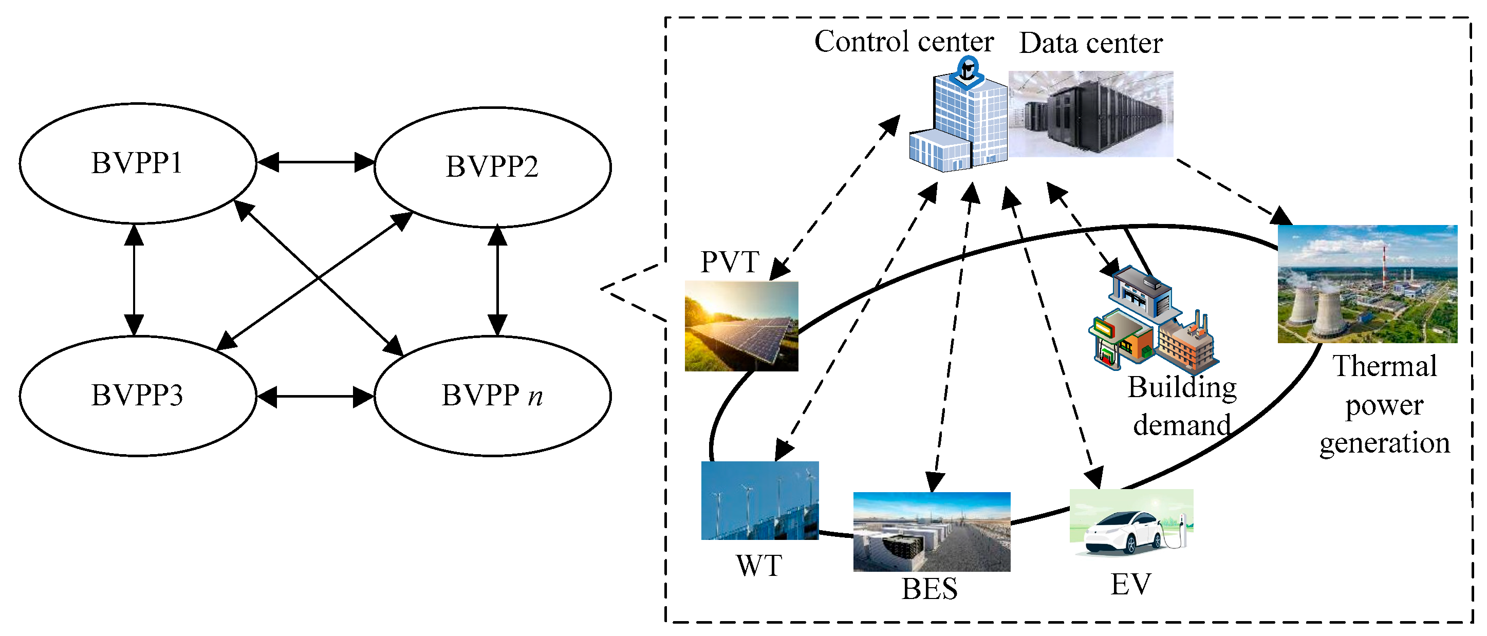
2.1. Distributed Computation–Electricity Trading Framework

With the advent of the cloud era and big data, multiple geographically distributed data centers are employed [2]. Due to the geographically distributed characteristic, the computation resources of the geodistributed BVPP system may meet many challenges: computation-intensive end-user devices, limited computing resources, spatiotemporal distribution, and so on. In addition to obtaining data from BVPP components for global coordination, computation resources are required among BVPP operators to exchange vital boundary information. Abundant opportunities for proactive demand response programs are provided with the rapid development of advanced emergence and proliferation of advanced smart meters. This would bring enormous burdens of communication and computation on energy-intensive communication devices. It is necessary to co-optimize the computation and electricity resources of BVPPs since computation resources play important roles in system operation. In centralized, layered, and distributed frameworks, reliable communication is inherent for cost-efficient systems and resource-efficient operations.
The N interconnected BVPPs that are geographically distributed are shown in Figure 1. WT, PVT, and BES are equipped within each BVPP to condition local solar-wind renewables to fulfill electricity demands. The deployment of advanced metering infrastructures and smart meters allows BVPPs to enter the electricity market. Thus, BVPPs can be operated as price-takers and allow end-users flexible loads to take part in demand response programs. Based on the management of the control center (the interconnection layer between the data center and the geographically distributed BVPPs), locally available computation–electricity resources can be fully utilized by BVPPs, thus achieving efficient resource management.
Using power lines and communication lines, distributed BVPPs can be cyber-interconnected. In this regard, networked BVPPs can compose a peer-to-peer trading group since the connected lines could be considered as the boundaries of the BVPPs. The mutual interactions of computation–electricity resources make these resources increasingly and intensively coupled. For example, during rush hours, a BVPP can receive many demand response requests, and its data center may seek computation resource assistance from surrounding data centers. In this paper, the main purpose is to optimize the computation–electricity trading behaviors among BVPPs cost-optimally, and locally available resources of resource-rich BVPPs are encouraged to be traded to resource-deficient BVPPs. The geo-distributed BVPPs here guarantee the supply–demand balance of the individual BVPP, and they can interact with each other BVPP through two-way communications over k time slots.

2.2. Computation–Electricity Allocations in Individual BVPPs

(1) Electricity procurement: BVPPs can buy electricity P buy , k , n from the electricity market with the electricity price μ buy , k , selling extra electricity P sell , k , n back to the distribution system operator with a feed-in tariff contract μ sell , k . The cost of electricity purchase C grid , k , n is presented as follows:
C grid , k , n = μ buy , k P buy , k , n Δ K μ sell , k P sell , k , n Δ K ,
0 P buy , k , n P buy , max ,
0 P sell , k , n P sell , max ,
where P buy , max and P sell , max are maximum power purchased and sold, ΔK is the time slot, and K is the overall scheduling period.
(2) Thermal Power Generation: As a traditional power generation system, thermal power units convert chemical energy into electricity by burning fossil fuels. The output of thermal power units requires us to guarantee the following constraints:
u i , k , n P i , n , min Th P i , k , n Th u i , k , n P i , n , max Th ,
R i , n d P i , k , n Th P i , k 1 , n Th R i , n u ,
where P i , k , n Th denotes the actual output of the thermal unit i at time k ; P i , n , min Th and P i , n , max Th are the minimum and maximum output of the thermal unit i ; u i , k , n is a binary variable, which presents the stop/start state of the thermal unit; R i , n d and R i , n u are the ramp-down and ramp-up power for the thermal unit i . Note that when P i , n , min Th is larger than R i , n d , (5) will make all the shutdown thermal power units fail to start. As such, (5) is rewritten as:
P i , k , n Th P i , k 1 , n Th u i , k 1 , n ( R i , n u R i , n , max u ) + R i , n , max u ,
P i , n , k 1 Th P i , k , n Th u i , k , n ( R i , n d R i , n , max d ) + R i , n , max d ,
where R i , n , max u and R i , n , max d , respectively, represent the maximum downhill and climbing speed of the thermal power i . To simplify,
R i , n , max u = R i , n , max d = 1 2 ( P i , n , min Th + P i , n , max Th ) .
The startup and shutdown of the thermal power unit must be maintained for a period of time to prevent damage caused by frequent actions. Thus,
t = k k + T S 1 ( 1 u i , t , n ) T S ( u i , k 1 , n u i , k , n ) ,
t = k k + T O 1 u i , t , n T O ( u i , k , n u i , k 1 , n ) ,
C i , k , n U H i ( u i , k , n u i , k 1 , n ) ,   C i , k , n U 0 ,
C i , k , n D J i ( u i , k 1 , n u i , k , n ) ,   C i , k , n D 0 ,
where T S and T O indicate the minimum shutdown and startup time of the unit; C i , k , n D and C i , k , n U , respectively, represent the cost of shutdown and startup of unit i at time k ; J i and H i indicate the unit cost of shutdown and startup of unit i . The thermal power unit cost function is presented as a quadratic function C Th , i , k , n ( P i , k , n Th ) , which is related to the output electrical power of the power unit:
C Th , i , k , n ( P i , k , n Th ) = a Th , i ( P i , k , n Th ) 2 + b Th , i P i , k , n Th + c Th , i ,
where a Th , i , b Th , i , and c Th , i indicate the coefficients of the quadratic function.
(3) Power Flexible Loads: Electric fans with adjustable speed and LED lights with adjustable brightness are typical power flexible loads [22]. With the advent of advanced information technology, these smart devices can be controlled via APP (iOS and Android) or remote control. In this case, the power consumption P p f , k , n of these loads is adjustable within the rated power range.
P p f , n , min P p f , k , n P p f , n , max ,
where P p f , n , min and P p f , n , max indicate the minimum and maximum power.
Additionally, to implement the expected work hours, the operational time of power flexible load P p f , k , n is required. As such, the lowest working value P n , exp must be guaranteed by the following operational constraints:
k T P p f , k , n P n , exp .
(4) Time-Flexible Loads: The wash and cleaning appliances in a BVPP (e.g., dryer, dish-washing machine, vacuum cleaner, and washing machine) are typical time-flexible loads. Nowadays, robotic vacuum cleaners have more contributions than others, which makes this popular appliance scheduled by demand–response programs. In this case, these appliances’ working times can be arranged while the power consumption P t f , k , n of these appliances is not adjustable. It means that they can operate on rated power P t f , 0 , n , as presented in the following constraint:
P t f , k , n = u t f , k , n P t f , 0 , n ,
where u t f , k , n is a binary variable, representing the state of the appliance.
A single time slot is not enough to fulfill the task. For example, to clean all dishes, washing machines need a long time. This type can be separated into two sub-types by considering the working/resting time sequences: time-continuous/discontinuous appliances. For the latter appliances, the operation state can be switched to ON/OFF while the overall running time guarantees the preset working value m m n :
k T u t f , k , n = m m n .
Different from the above appliance, the appliance which is time-continuous must continuously work to achieve the preset working value m n :
t = k k + m n u t , n m n ( u t f , k + 1 , n u t f , k , n ) .
(5) Temperature Flexible Loads: Heating load, including spacing heating, heating, ventilation, and air conditioning (HVAC), is a typical temperature flexible load. A common feature of these appliances is that the operational temperature can be adjusted according to the man-made setting. R-C thermodynamics have been extensively used to govern temperature changes, which are jointly decided via outside temperature, supply air temperature of HVAC, etc. The supply air temperature of HVAC directly determines the energy consumption of the temperature flexible loads.
Consider the single-area thermal network shown in Figure 2, where the red frames indicate the walls of the building. An R-C thermal network is developed to describe the thermal dynamic of the building climate by representing heat storage as thermal capacitance and heat transfer as thermal resistance. The thermal potential nodes are connected through thermal capacitors to the ground and thermal resistors to the contiguous nodes [23]. The peripheral wall node is interconnected with the outside air node via two-series resistance R W , i / 2 and R out , i . The internal wall nodes are interconnected with a zone node via two series resistors with resistances R W , i / 2 and R in , i . As window mass is much less than wall mass, its thermal capacitance can be ignored. The window i can be modeled as pure resistance R win , i , which is parall with the thermal resistance of its wall.
R W , i = R value wall A W i , R in , i = R value in A W i , R out , i = R value out A W i , R win , i = R value in + R value glass + R value out A win i ,
where R W , i , R out , i , and R in , i represent the thermal resistance of wall i ( i = 1 , 2 , 3 , 4 ) for conduction heat transfer, external convective heat transfer, and internal convective heat transfer; R value wall and R value glass indicate the R -value of wall and glass window; R value out and R value in , respectively, indicate the R -value of external surface film and internal surface film; A W i and A win i , respectively, represent the total area of wall i and the total area of window i .
The state space expression of Figure 2 is expressed as:
C Z , 1 , n d T Z , 1 , n d t = c a m ˙ Z , 1 , n ( T S , 1 , n T Z , 1 , n ) + T W , 1 , n T Z , 1 , n R W , 1 , n 2 + R in , 1 , n + T W , 2 , n T Z , 1 , n R W , 2 , n 2 + R in , 2 , n + T W , 3 , n T Z , 1 , n R W , 3 , n 2 + R in , 3 , n + T W , 4 , n T Z , 1 , n R W , 4 , n 2 + R in , 4 , n + T out T Z , 1 , n R win , 1 , n + ϵ win 1 A win 1 Q r a d 1 + Q ˙ i n t 1 , C W , 1 , n d T W , 1 , n d t = T Z , 1 , n T W , 1 , n R W , 1 , n 2 + R in , 1 , n + T out T W , 1 , n R W , 1 , n 2 + R out , 1 , n + α W 1 A W 1 Q r a d 1 , C W , 2 , n d T W , 2 , n d t = T Z , 1 , n T W , 2 , n R W , 2 , n 2 + R in , 2 , n + T out T W , 2 , n R W , 2 , n 2 + R out , 2 , n , C W , 3 , n d T W , 3 , n d t = T Z , 1 , n T W , 3 , n R W , 3 , n 2 + R in , 3 , n + T out T W , 3 , n R W , 3 , n 2 + R out , 3 , n , C W , 4 , n d T W , 4 , n d t = T Z , 1 , n T W , 4 , n R W , 4 , n 2 + R in , 4 , n + T out T W , 4 , n R W , 4 , n 2 + R out , 4 , n ,
where C Z , 1 , n = c a m a , 1 is the thermal capacitance of zone 1 and C W , i , n = c w m w , i is the thermal capacitance of wall i ( c w and c a are the specific heat capacity of wall and air; m a , 1 and m w , i are the air mass in zone 1 and the wall mass); T S , 1 , n is the supply air temperature of HVAC entering zone 1; T W , i , n and T Z , 1 , n are the temperature of wall i and zone 1; T out is the outside ambient temperature; m ˙ Z , 1 , n is the mass flow rate of air entering zone 1 (airflow); Q ˙ r a d 1 is the internal heat gain (from electrical devices, etc.) in zone 1; Q ˙ r a d 1 is the solar radiative heat flux density that radiates into node 1; ϵ win 1 is the glass transmissivity of window in zone 1; α W 1 is the solar radiation absorption coefficient.
BVPPs can achieve demand response by setting HVAC temperatures to ensure reliable and safe operation, while elastic temperature regulation can deviate from its optimal temperature, resulting in discomfort costs C HVAC , k , n that deviate from their preferred temperature level T exp , n :
C HVAC , k , n = μ HVAC ( T W , 4 , n T exp , n ) 2 ,
where μ HVAC is the unit discomfort cost of temperature deviation.
(6) Electric Vehicles: Electric vehicle (EV) AC slow/DC fast charging is implemented and are defined via its maximum charging power. BVPPs deal with the EV charging mode reasonably according to the charging urgency. Charging stations arrange DC fast charging for EVs with high urgency, and ensure the charging results meet the expected state of charge when they travel. The charging urgency is defined as the ratio of maximum charging time to the duration of stay:
α i , n = T i , n , A T i , n , w T i , n , A = ( S i , n , e S i , n , b ) Q n , e P n , ch , max EV , AC ,
where α i , n denotes the charging urgency of EV i ; when α i , n 0.1 , the charging of EV i is urgent, and DC fast charging is chosen; otherwise, AC slow charging is chosen; T i , n , A denotes the duration of AC slow charging from maximum power to expected state of charge (SOC) of EV i ; T i , n , w represents the duration of stay of EV i , which is defined by daily travel time and daily return time; P n , ch , max EV , AC indicates the maximum charging power of AC slow charging pile; S i , n , b is the SOC at the time of the return of EV i ; S i , n , e presents the expected SOC of EV i ; Q n , e is the battery capacity.
While the daily travel time and daily return time of EVs are assumed to follow the standard normal distribution, the daily mileage and the expected SOC are assumed to follow the lognormal distribution [1,24]. The SOC at the time of the return of EV i is calculated:
S i , n , b = S i , n , e w 100 100 × d i , n Q n , e ,
where d i , n is the daily mileage of EV i , and w 100 is the consume electricity for 100 km of EV.
Using the Monte Carlo sampling method, the travel model (expected SOC, the arrangements of AC slow/DC fast charging) of EVs can be obtained from (22) and (23), which can be used to help arrange AC slow/DC fast charging.
Each EV only charges or discharges at the same time. The constraints of charge/discharge are present as follows:
μ i , k , n , ch EV , AC + μ i , k , n , dis EV , AC y i , n AC μ i , k , n , ch EV , DC + μ i , k , n , dis EV , DC y i , n DC ,   k T F ,
where μ i , k , n , ch EV , AC and μ i , k , n , dis EV , AC represent the AC slow charging and discharging state of EV i , respectively; μ i , k , n , ch EV , DC and μ i , k , n , dis EV , DC represent the DC fast charging and discharging state of EV i , respectively; y i , n AC and y i , n DC denote the charging method of EV i , e.g., EV i is DC fast charging when y i , n DC = 1 and AC slow charging when y i , n AC = 1 ; T F is the set of free time of EV.
The power constraint of EV is presented as follows:
0 P i , k , n , ch EV , AC μ i , k , n , ch EV , AC P n , ch , max EV , AC 0 P i , k , n , dis EV , AC μ i , k , n , dis EV , AC P n , dis , max EV , AC 0 P i , k , n , ch EV , DC μ i , k , n , ch EV , DC P n , ch , max EV , DC 0 P i , k , n , dis EV , DC μ i , k , n , dis EV , DC P n , dis , max EV , DC ,
where P n , ch , max EV , AC and P n , dis , max EV , AC denote maximum AC slow charging and discharging; P n , ch , max EV , DC and P n , dis , max EV , DC denote maximum DC fast charging and discharging. The ramp constraint of DC fast charging is as follows:
P n , sub EV , DC P i , k , n EV , DC P i , k + 1 , n EV , DC P n , sub EV , DC ,
where P n , sub EV , DC is the ramp power. The constraints of SOC are presented as follows:
S i , n , min S i , k , n S i , n , max S i , n , TS S i , n , e S i , k + 1 , n = S i , k , n + P i , k , n EV Δ T / Q e ,
where S i , k , n represents the actual SOC of EV i at time k ; S i , n , max and S i , n , min indicate the upper and lower bound of SOC of EV i ; P i , k , n EV is the actual power of EV i charging at time k , positive when charging and negative when discharging; S i , n , TS is the SOC at the travel time of EV i .
The battery degradation cost C EV , b , n is presented as follows:
C EV , b , n = λ EV k = 1 K i = 1 N EV [ P i , k , n , ch EV , AC + P i , k , n , dis EV , AC + P i , k , n , ch EV , DC + P i , k , n , dis EV , DC ] Δ K ,
where λ EV is the unit degradation cost.
(7) Battery Energy Storage: Frequent charging P n , k , ch BES and discharging P n , k , dis BES of BES leads to a certain degree of wear. The degradation cost of a battery, C BES , n , can be calculated as follows:
C BES , n = μ BES k = 1 K n = 1 N BES ( P n , k , ch BES + P n , k , dis BES ) Δ K ,
where μ BES indicates the unit cost of average/amortized degradation. The constraints limiting the SOC and BES charging/discharging are presented as follows:
S O C n , k BES = S O C n , k 1 BES + η ch BES P n , k 1 , ch BES Δ K E n R P n , k 1 , dis BES Δ K η dis BES E n R ,
S O C min BES S O C n , k BES S O C max BES ,
x n , k , ch BES + x n , k , dis BES 1 0 P n , k , ch BES P n , k , ch BES P ch , max BES 0 P n , k , dis BES P n , k , dis BES P dis , max BES ,
where E n R is the BES capacity; S O C n , k BES is the current SOC; η ch BES and η dis BES are the efficiencies of BES charging and discharging, respectively; S O C min BES and S O C max BES are the minimum and maximum SOC; P ch , max BES and P dis , max BES are charging and discharging limits; x n , k , ch BES and x n , k , dis BES represent the charging and discharging state of SOC.
(8) Data Center: Different from the simple strategy of first-come, first-served queuing, the concurrent process of BVPP data centers is adopted for executing multiple tasks synchronously. The data center would decide whether to process the data load from the network requests in each time period. When the data load is to be executed, it is allocated to the server and sent back to end-users after completion. Otherwise, it will enter the waiting queue. Such proactive data center demand–response has remarkable strengths in the following aspects:
(1)
Flexible load balancing: BVPP supply–demand fluctuates, and the data load arriving time is centralized. By fully taking into account available resources and data load, data center buildings can perform flexible demand–response for renewable energy accommodation.
(2)
Cost-effective responsiveness: At the expense of a certain degree of user satisfaction, the allocation of processing servers and resources can be quickly adjusted to accommodate the pricing/incentive signals.
The energy consumption of BVPP data centers is close to the ratio of the server’s work/idle. Here, the number of servers is used to describe the resource capacity of BVPP data centers and quantify the corresponding energy consumption.
Constraints (33) limit the standby server for the data load.
i L i , k , n D n ( 1 q n ) ,
where L i , k , n is the number of occupied serves; D n is the maximum number of serves in BVPP data centers; q n indicates the standby server ratio of BVPP data centers.
Constraint (34) limits the resource allocation of computing in parallel.
S DT , i , n , min I i , k , n L i , k , n S DT , i , n , max I i , k , n ,
where S DT , i , n , min and S DT , i , n , max are the minimum and maximum assigned serves; I i , k , n is the processing status of data load, i.e., 0 is not processed and 1 is processing.
Constraint (35) indicates that when the i th data load can be accomplished without being delayed or within the present time, u i = 0 .
u i , n = 0 ,   if   A DT , i , n = k [ k i , k i + h i ] L i , k , n ,
where A DT , i , n is the data load; u i , n is the accomplishing status of data load by assigned servers, i.e., u i , n = 1 indicates that the data load i cannot be accomplished within the required time. u i , n = 0 means that the data load i can be accomplished without being delayed.
Constraint (36) limits the data load i is handled timely under the present time and quits the queue to desert the server resources.
I i , k , n = 0 ,   if   u i , n = 0 .
Constraint (37) indicates that no server would be assigned when the data load i has not arrived in the data center yet.
I i , k , n = 0 ,   k [ 0 , k i 1 ] .
Constraint (38) limits the processing data load number that needs to be equated to the total data load number.
i k L i , k , n = i A DT , i , n .
Obviously, when the number of assigned servers is larger, the corresponding IT energy consumption is larger simultaneously. The energy consumption of IT equipment P I T , k , n can be described as follows:
P I T , k , n = c k , n P I T , n , max + l n ( 1 c k , n ) P I T , n , max ,
where l n is the ratio of the idle to peak energy consumption, and c k , n can be calculated as the ratio of the assigned servers to the total number of serves:
c k , n = i L i , k , n D n .
The data center energy consumption LDC,k,n in a BVPP includes IT energy consumption P I T , k , n and energy consumption of the ancillary equipment P A , k , n :
L DC , k , n = P A , k , n + P I T , k , n .
Here, the definition of power usage effectiveness (PUE), which is reflected in the ratio of the total energy consumption to IT energy consumption, is introduced as follows:
P U E n = L D C , k , n P I T , k , n .

2.3. Peer-to-Peer Computation–Electricity Trading among BVPPs

It is essential for multi-BVPPs to trade computation and electricity, which can improve the operational economy and resource utilization. Each BVPP here could consult with other networked BVPPs for the computation–electricity trading number T r , k , n , n a and the corresponding payment C r , k , n , n a . In the multi-BVPP system, electricity and data center servers are two types of trading resources and are simply defined as “p” and “u”. The computation–electricity trading and the corresponding payment among BVPPs must guarantee the following constraints of market clearing:
T r , k , n , n a + T r , k , n a , n = 0 r = p , u ,
C r , k , n , n a + C r , k , n a , n = 0 r = p , u .
Each BVPP has its own balance constraints:
L k , n + L DTtot , k , n + c a m ˙ Z , 1 , n ( T S , 1 , n T Z , 1 , n ) / η H V A C = P WT , k , n + P PVT , k , n + P buy , k , n P sell , k , n + i = 1 N Th P i , k , n Th + P n , k , dis BES P n , k , ch BES + i = 1 N EV ( P i , k , n , dis EV , AC P i , k , n , ch EV , AC + P i , k , n , dis EV , DC P i , k , n , dis EV , DC ) n a N \ n T e , k , n , n a ,
where ηHVAC is the electrical–thermal efficiency, and P PVT , k , n and P WT , k , n are outputs of PVT and WT.
The amount of server D n includes the occupied server i L i , k , n , the idle server L f , k , n , and the used server T u , i , k , n , n a for trading:
D n = i L i , k , n + L f , k , n + n a N \ n i T u , i , k , n , n a .
The total energy consumption L DTtot , k , n of BVPP data centers includes the individual energy consumption L DT , k , n and the energy consumption T s , k , n , n a incurred from trading:
L DTtot , k , n = L DT , k , n + n a N \ n T s , k , n , n a .
In this case, constraints (33), (35), and (38) are rewritten as follows:
i L i , k , n + n N \ n a i T u , i , k , n , n n D n ( 1 q n ) ,
u i , n = 0 ,   if   A DT , i , n = k [ k i , k i + h i ] L i , k , n + n a N \ n T u , i , k , n a , n ,
i k L i , k , n + n a N \ n T u , i , k , n a , n = i A DT , i , n .
The purpose of each BVPP operator is to minimize the total operating cost of individual BVPPs’ C non , n , including the power purchase cost C grid , k , n , generation cost i = 1 N Th C Th , i , k , n , discomfort cost of users C HVAC , k , n , and battery degradation cost of EV C EV , b , n and BES C BES , n :
C non , n = k K ( C grid , k , n + i = 1 N Th C Th , i , k , n + C HVAC , k , n ) + C EV , b , n + C BES , n .

3. Proposed Solution Methodology

The peer-to-peer computation–electricity trading (1)–(11) of BVPPs cannot be solved easily via standard commercial solvers since there are computation–electricity couplings, conflicts of interests, etc. Technical parameters and multiparty operating states are required when performing coordinated peer-to-peer computation–electricity trading. Nevertheless, geodistributed BVPPs are generally not governed by only a single entity/manager. Therefore, this paper first develops a transactive bargaining framework to promote mutually beneficial trading among BVPPs. Then, the computation–electricity trading problem is decomposed into multiple BVPP-based decision-making level subproblems, which can be solved iteratively using a fully distributed algorithm with only limited information sharing.

3.1. Cooperative Bargaining

BVPPs can determine sharing amounts and methods, which is the original meaning of cooperative bargaining. A bargain problem between two-person includes:
(1)
A feasibility set F, a usually assumed convex closed subset of 2 that is often assumed to be convex, the elements of which are explained as agreements.
(2)
A disagreement, or threat, point d = ( d 1 , d 2 ) , where d 1 and d 2 are the payoffs to players 1 and 2. If these two players cannot reach a mutual agreement, they are guaranteed to receive the payoffs.
When the agreements in F are preferable for both parties to the disagreement point, the bargaining problem is nontrivial. For the bargaining problem, one solution is to select an agreement in F. For the properties desired for the final agreement point, there have been many solutions proposed based on slightly different assumptions. In [25,26], certain axioms that the solution should be satisfied were proposed by John Forbes Nash Jr. That is, invariant to equivalent utility representations, symmetry, independence of irrelevant alternatives, and Pareto optimality. It has been shown that the solutions satisfying the above axioms are just the points in F that maximize the expression:
max u 1 , u 2 ( u 1 d 1 ) ( u 2 d 2 )   s . t . ( u 1 , u 2 ) U ;   ( u 1 , u 2 ) > ( d 1 , d 2 ) ,
where ui and di (i = 1, 2) are represented as the payoffs from the disagreement point of two players; U is a set, which is convex feasibility, and the elements of U can be explained as agreements; the product of the two excessive benefits ( u 1 d 1 ) ( u 2 d 2 ) is usually called the Nash product.
Self-interested BVPP operators negotiate via mutually beneficial agreements with each other, which makes both players more advantageous than the disagreement points. Each BVPP would bargain with other BVPPs for the computation–electricity number and the corresponding payment. The extra defrayment C T , n to other BVPPs is calculated as follows:
C T , n = r n a N \ n k K C r , k , n , n a .
Then, the overall cost C tot , n of BVPP n can be calculated as follows:
C tot , n = k K ( C grid , k , n + i = 1 N Th C Th , i , k , n + C HVAC , k , n ) + C EV , b , n + C BES , n + C T , n .
For each operator, it is rational to improve its computation–electricity utilization by implementing cost-optimal computation–electricity trading. It is certain that every BVPP will not cooperate if their cost cannot be reduced.
C tot , n C wt , n ,
where C wt , n is the disagreement point. It presents the minimum value of the C non , n , which is obtained for BVPP n without trading computation–electricity with other BVPPs.
The proposed computation–electricity trading problem can be presented as follows:
max n N ( C wt , n C tot , n )   s . t .   ( 1 ) ( 54 ) .
For problem (55), the involved decision variables could be separated into two decoupled sets: computation–electricity allocation and trading payment. Therefore, the computation–electricity trading problem (55) is equally resolved into two subproblems: social computation–electricity allocation (56) and payoff allocation (57):
min n N C non , n   s . t .   ( 1 ) ( 42 ) , ( 43 ) , ( 45 ) ( 53 ) ,
max n N ( C wt , n C non , n C T , n )   s . t .   ( 44 ) , ( 54 ) ,
where C non , n is the optimal value obtained from the subproblem (56).
Proof: For the provided optimal computation–electricity allocation decisions, the optimal trading payment decisions from subproblem (57) are calculated as follows:
C T , n = C wt , n C non , n n N ( C wt , n C non , n ) / N .
By substituting (18) into problem (15), the optimal objective yields
n N ( C wt , n C non , n ) / N N .
Thus, it is proved that the social cost of all BVPPs in subproblem (56) can be minimized via problem (55). By solving subproblems (56) and (57) sequentially, optimal computation–electricity trading solutions can be obtained.
The proof is completed.

3.2. Model Reformulation

For the aim of computation complexity reduction, the nonlinear building model (20) is linearized around this equilibrium point where the system is working most of the time. Due to the small temperature range, this linearization does not introduce significant errors [23]. Then, the state-space-based linear building model is discretized:
x k + 1 , n = A x k , n + B u k , n ,
y k , n = C x k , n ,
where x k , n is the state vector, representing the node temperature; y k , n is the system output vector; u k , n represents the controllable HVAC input.
For nonlinear constraints (36) and (49), the so-called big-M method is utilized by selecting the relatively large value M n and small value m n :
A i , n k [ k i , k i + h i ] L i , k , n + n a N \ n T u , i , k , n a , n M n u i , n ,
A i , n k [ k i , k i + h i ] L i , k , n + n a N \ n T u , i , k , n a , n m n u i , n ,
I i , k , n M n u i , n 0 , k [ k i + h i + 1 , K ] ,
where M n and m n represent the relatively large and small parameters.

3.3. Distributed Algorithm

The couplings of subproblems (56) and (57) are the computation–electricity trading constraint (43) and the corresponding payment constraint (44). To protect information privacy, a fully distributed algorithm is developed to solve the decomposed subproblems, which are shown in Algorithm 1. It can be found that distributed self-interested BVPPs optimally maximize their profit and share necessary trading information with surrounding BVPPs.
As binary variables are introduced, the convergence, existence, and uniqueness of the problem (55) can be guaranteed: (1) the bargaining problem has inherent Pareto efficiency and convexity properties in nature [25,26]; (2) some binary variables can be eliminated based on optimization techniques. For example, it was proved in [23] that charging/discharging variables would always be mutually exclusive since the product of charging/discharging efficiency is less than 1; (3) after several iterations, the binary variables will no longer change, coercing the minimum value of the problem gradually to approach the feasible region. The details of this proof can be found in [27].
Algorithm 1: Distributed Algorithm for Solving (56) and (57).
1:Set the parameters of energy generation, electricity demand response appliances, and storage of the multi-BVPP system
2:Provide iteration index i t = 0 and tolerances δ 1 and δ 2 . Initialize Lagrangian multipliers y t ,   y c , and step size d y ,   d c
3:Combine local constraints (1)–(42) and (45)–(53) and the following Lagrangian function for objective (56); each BVPP solves the social electricity allocation subproblem in parallel.
T r , k , n , n a i t + 1 = argmin C non , n + d t , r , n , n a 2 k K n a N \ n | | T r , k , n , n a T r , k , n , n a i t + T r , k , n a , n i t , aver + y r , k , n , n a i t | | 2 2 .
4:Calculate and check whether the residual is less than the preset tolerance:
max k K n a N \ n | | T r , k , n , n a i t + 1 + T r , k , n a , n i t + 1 | | 2 2 δ 1 .
Once it is satisfied, the iteration stops. Otherwise, each BVPP updates its y t :
y t , r , k , n , n a i t + 1 = y t , r , k , n , n a i t + T r , k , n , n a i t + 1 , aver .
5:Set the iteration index to i t = i t + 1 , and repeat steps 3 and 4 for each BVPP until the conditions for stopping are guaranteed.
6:Combine with local constraints (54) and the following Lagrangian function for objective (57); each VPP parallelly solves the payment bargaining subproblem:
C r , n , n a i t + 1 = argmin { ln ( C w t , n C non , n C T , n ) + d c , r , n , n a 2 n a N \ n | | C r , n , n a C r , n , n a i t + C r , n a , n i t , aver + y c , r , n , n a i t | | 2 2 }
7:Calculate and check whether the residual is less than the preset tolerance:
max n a N \ n | | C r , n , n a i t + 1 + C r , n a , n i t + 1 | | 2 2 δ 2 .
Once it is satisfied, the iteration stops. Otherwise, each BVPP updates its y c :
y c , r , n , n a i t + 1 = y c , r , n , n a i t + C r , n , n a i t + 1 , aver .
8:Set the iteration index to i t = i t + 1 , and repeat steps 6 and 7 for each BVPP until the conditions for stopping are guaranteed.

4. Case Studies

4.1. System Description

In this section, a three-BVPP system is used to prove the effectiveness of the proposed distributed transactive electricity trading methodology. The schematic diagram of the BVPP system is given in Figure 1. The feed-in price is given as 0.01 $/kWh, and the related electricity price is obtained from [28]. The parameters of base energy consumptions, storages, and generations of three BVPPs are obtained from [1,2,22].
To verify the effective and superior performances of the proposed methodology, three comparative schemes with different trading schemes are given as follows:
(1)
Scheme 1 presents the proposed distributed transactive multi-resource trading in Section 2 and Section 3;
(2)
Scheme 2 presents the distributed transactive multi-resource trading without considering the server trading;
(3)
Scheme 3 presents the multiple BVPP scheduling without considering the multi-resource trading.
The computation-electricity trading is performed every 1 h over a 24 h period, which also can be directly applied to other time scales according to the actual requirements.

4.2. Performance Comparison

The daily computation-electricity trading curves among BVPPs in schemes 1 and 2 are shown in Figure 3 and Figure 4, respectively. For schemes 1–3, the electricity purchase and server utilization of BVPPs in schemes 1–3 are drawn in Figure 5 and Figure 6, respectively. From Figure 3 and Figure 4, it can be found that all three BVPPs trade the computation-electricity resources interactively with each other across the 24 h operation horizon. The renewable outputs of BVPP 3 during hours 1–12 are relatively higher than BVPPs 1 and 2. Thus, BVPP 3 sells its excessive energy to BVPPs 1 and 2. Since the renewable power supply suddenly dropped in hours 11–24, BVPP 3 has to purchase electricity from the other two BVPPs. Note that although extra payments are required for the electricity trading among BVPPs, the trading enables renewable accommodation instead of electricity selling back to the electricity market. Thus, BVPP 2 in scheme 1 purchases less electricity from the market than other schemes, decreasing its operating costs.
When the computation resource is shortage in some BVPPs, the computation resource-rich BVPP 1 can trade its server to surrounding computation resource-deficient BVPPs 2 and 3. Thus, the data processing capability of the BVPP system can be improved. As shown in Figure 6, in schemes 2 and 3 without computation trading, the computation in BVPP 2 stays at a high utilization in hours 12–16. In scheme 1, the average computation utilization of BVPPs 1 and 2 are reduced by offloading requests to the surroundings.
In schemes 1–3, the storage outputs of three BVPPs are shown in Figure 7 and Figure 8. It is not hard to find that, the proposed methodology in scheme 1 can achieve optimal synergies of internal computation-electricity allocations within each BVPPs and the external multilateral computation-electricity trading among networked BVPPs. While BES and EV charging during morning and noon hours, abundant renewable generations are the main energy sources for energy supplies. There is a sharp decrease in renewable generations during the hour 17–24, and the BES in scheme 1 rapidly increases to meet the rising demands. In scheme 3, batteries stay undercharged during hours 11–14 and provide an additional inverse discharging.
Figure 9 and Figure 10 present the daily electricity supply demand balance and the optimized electricity load curve in schemes 1 and 3. Though during hours 11–15 (solar energy) and hours 1–10 (wind energy), renewable generations are abundant, the electricity price during the peak hours 11–20 is higher. It can be found that the elastic loads of all BVPPs are shifted from on-peak time periods to off-peak time periods. For instance, during morning hours, more renewable energy is consumed and during on-peak hours, less electricity is purchased.
The operating costs and the corresponding payments obtained with and without trading are listed in Table 1 for comparison. It is not hard to find that, the system operation cost with the computation-electricity trading is decreased by up to 8.78%. In detail, every BVPP benefits through computation-electricity trading by considering the cost and payment influences. It is because that profit seeking BVPPs deliver their power to other BVPPs rather than selling back to the electricity market. The operating costs of all BVPPs have been decreased by 8.98%, 2.25%, and 15.64% compared with scheme 3, which verifies the effectiveness and superiority of the proposed scheme.
The detailed comparisons of the operating costs, electricity procurement, battery degradation costs, thermal power unit cost, and discomfort costs in schemes 1–3 are provided in Table 2. It can be found that scheme 1 can satisfy daily electricity supply demand balance and data processing with less power purchase compared with schemes 2 and 3. Compared with scheme 2, the cost of system operation of scheme 1 is reduced by 1.52%. As for the discomfort cost, the three schemes keep the same value, which means that the temperature of the HVAC is not affected by the computation-electricity trading.
Based on the above analysis, the method proposed in this paper can provide diversified renewable energy utilization paths through the synergy between storages. As a result of the peer-to-peer computation-electricity trading, BVPPs in schemes 1 and 2 tend to share their available demand response resources and storage to maximize renewable utilization. In a word, case studies confirm that the merits of the developed methodology on cost-efficient computation-electricity management, particularly on the enhancements of computation resource utilization and operational economy.

5. Conclusions

In this paper, a distributed transactive computation-electricity trading framework for the optimal synergies of heterogeneous BVPPs is proposed. The multiple BVPP computation-electricity trading problem has been decomposed into social computation-electricity allocation and payoff allocation subproblems. It could be found from case studies that:
(1)
As a result of proactive computation-electricity trading, locally available resources of resource-rich BVPPs are encouraged to be traded to the resource-deficient BVPPs with satisfactory payoff.
(2)
The proposed methodology achieves fully distributed computation-electricity trading by sharing only necessary information, therefore preserving the resource-autonomy and information privacy.
(3)
The proposed distributed transactive trading scheme can outperform others on system resource utilization and operational economy, which has huge development and application potentialities in urban/community building system.
Energy storage from BVPP can facilitate power system operation by providing various market-remunerated and regulated services including ancillary services, energy services, and capacity services. Market mechanisms and regulatory frameworks are two powerful factors in cost recovery and asset profitability, which should be redefined and refined to eliminate biases and market barriers. Additionally, while the multi-energy system is the mainstream, electricity is the main energy carrier of this paper, which is the research limitation and will be our future works.

Author Contributions

Conceptualization, W.K and D.H.; methodology, X.C.; software, W.C.; formal analysis, S.D.; investigation, W.X.; resources, Z.G.; data curation, W.K.; supervision, D.X.; writing—original draft, Z.G.; writing—review & editing, W.C. and D.X. All authors have read and agreed to the published version of the manuscript.

Funding

This research was funded by the China Postdoctoral Science Foundation funded project under Grant 2021M692992.

Data Availability Statement

The data presented in this study are available on request from the corresponding author. The data are not publicly available due to privacy.

Conflicts of Interest

Authors Zhiping Gao, Wenwen Kang, Xinghua Chen, Sheng Ding ans Wei Xu were employed by the company Hubei Branch of State Power Investment Group Co., Ltd. Author Degang He was employed by the company Institute of New Energy. The remaining authors declare that the research was conducted in the absence of any commercial or financial relationships that could be construed as a potential conflict of interest.

References

  1. Liu, L.; Xu, D.; Lam, C.S. Two-layer management of HVAC-based multi-energy buildings under proactive demand response of Fast/Slow-charging EVs. Energy Convers. Manag. 2023, 289, 117208. [Google Scholar] [CrossRef]
  2. Xu, D.; Xiang, S.; Bai, Z.; Wei, J.; Gao, M. Optimal multi-energy portfolio towards zero carbon data center buildings in the presence of proactive demand response programs. Appl. Energy 2023, 350, 121806. [Google Scholar] [CrossRef]
  3. Naval, N.; Yusta, J.M. Virtual power plant models and electricity markets—A review. Renew. Sust. Energ. Rev. 2021, 149, 111393. [Google Scholar] [CrossRef]
  4. Buildings as Power Plants. Available online: https://www.ctvc.co/buildings-as-power-plants/ (accessed on 2 December 2022).
  5. Chen, Y.; Mei, S.; Zhou, F.; Low, S.H.; Wei, W.; Liu, F. An energy sharing game with generalized demand bidding: Model and properties. IEEE Trans. Smart Grid 2020, 11, 2055–2066. [Google Scholar] [CrossRef]
  6. Zhang, J.; Che, L.; Wan, X.; Shahidehpour, M. Distributed hierarchical coordination of networked charging stations based on peer-to-peer trading and EV charging flexibility quantification. IEEE Trans. Power Syst. 2022, 37, 2961–2975. [Google Scholar] [CrossRef]
  7. Cui, S.; Wang, Y.W.; Shi, Y.; Xiao, J.W. A new and fair peer-to-peer energy sharing framework for energy buildings. IEEE Trans. Smart Grid 2020, 11, 3817–3826. [Google Scholar] [CrossRef]
  8. Chen, L.; Liu, N.; Li, C.; Wang, J. Peer-to-peer energy sharing with social attributes: A stochastic leader–follower game approach. IEEE Trans. Ind. Inform. 2021, 17, 2545–2556. [Google Scholar] [CrossRef]
  9. Haggi, H.; Sun, W. Multi-round double auction-enabled peer-to-peer energy exchange in active distribution networks. IEEE Trans. Smart Grid 2021, 12, 4403–4414. [Google Scholar] [CrossRef]
  10. Morstyn, T.; Teytelboym, A.; Mcculloch, M.D. Bilateral contract networks for peer-to-peer energy trading. IEEE Trans. Smart Grid 2019, 10, 2026–2035. [Google Scholar] [CrossRef]
  11. Xu, S.; Zhao, Y.; Li, Y.; Zhou, Y. An iterative uniform-price auction mechanism for peer-to-peer energy trading in a community microgrid. Appl. Energy 2021, 298, 117088. [Google Scholar] [CrossRef]
  12. Xu, D.; Zhou, B.; Liu, N.; Wu, Q.; Voropai, N.; Li, C. Peer-to-peer multienergy and communication resource trading for interconnected microgrids. IEEE Trans. Ind. Inform. 2020, 17, 2522–2533. [Google Scholar] [CrossRef]
  13. Wei, X.; Liu, J.; Xu, Y.; Sun, H. Virtual power plants peer-to-peer energy trading in unbalanced distribution networks: A distributed robust approach against communication failures. IEEE Trans. Smart Grid 2023, 2023, 3308101. [Google Scholar] [CrossRef]
  14. Li, J.; Xu, D.; Wang, J.; Zhou, B.; Wang, M.H.; Zhu, L. P2P multigrade energy trading for heterogeneous distributed energy resources and flexible demand. IEEE Trans. Smart Grid 2023, 14, 1577–1589. [Google Scholar] [CrossRef]
  15. Yang, Q.; Wang, H.; Wang, T.; Zhang, S.; Wu, X.; Wang, H. Blockchain-based decentralized energy management platform for residential distributed energy resources in a virtual power plant. Appl. Energy 2021, 294, 117026. [Google Scholar] [CrossRef]
  16. Zhang, Y.; Chen, Z.; Ma, K.; Chen, F. A decentralized IoT architecture of distributed energy resources in virtual power plant. IEEE Internet Things J. 2022, 10, 9193–9205. [Google Scholar] [CrossRef]
  17. Ullah, M.H.; Park, J.D. Peer-to-peer energy trading in transactive markets considering physical network constraints. IEEE Trans. Smart Grid 2021, 12, 3390–3403. [Google Scholar] [CrossRef]
  18. Xu, D.; Wu, Q.; Zhou, B.; Li, C.; Bai, L.; Huang, S. Distributed multi-energy operation of coupled electricity, heating, and natural gas networks. IEEE Trans Sustain. Energy 2019, 11, 2457–2469. [Google Scholar] [CrossRef]
  19. Xia, Y.; Xu, Q.; Tao, S.; Du, P.; Ding, Y.; Fang, J. Preserving operation privacy of peer-to-peer energy transaction based on enhanced benders decomposition considering uncertainty of renewable energy generations. Energy 2022, 250, 123567. [Google Scholar] [CrossRef]
  20. Xiao, X.; Wang, F.; Shahidehpour, M.; Zhai, Y.; Zhou, Q. Peer-to-peer trading in distribution system with utility’s operation. CSEE J. Power Energy Syst. 2021. in print. [Google Scholar] [CrossRef]
  21. Samende, C.; Cao, J.; Fan, Z. Multi-agent deep deterministic policy gradient algorithm for peer-to-peer energy trading considering distribution network constraints. Appl. Energy 2022, 317, 119123. [Google Scholar] [CrossRef]
  22. Xu, D.; Zhong, F.; Bai, Z.; Wu, Z.; Yang, X.; Gao, M. Real-time multi-energy demand response for high-renewable buildings. Energy Build. 2023, 281, 112764. [Google Scholar] [CrossRef]
  23. Xu, D.; Zhou, B.; Wu, Q.; Chung, C.Y.; Li, C.; Huang, S.; Chen, S. Integrated modelling and enhanced utilization of power-to-ammonia for high renewable penetrated multi-energy systems. IEEE Trans. Power Syst. 2020, 35, 4769–4780. [Google Scholar] [CrossRef]
  24. Tan, J.; Wang, L. Integration of plug-in hybrid electric vehicles into residential distribution grid based on two-layer intelligent optimization. IEEE Trans. Smart Grid 2014, 5, 1774–1784. [Google Scholar] [CrossRef]
  25. Nash, J.F., Jr. The bargaining problem. Econom. J. Econom. Soc. 1950, 18, 155–162. [Google Scholar] [CrossRef]
  26. Thomson, W. Cooperative models of bargaining. Handb. Game Theory 1994, 2, 1237–1284. [Google Scholar]
  27. Boyd, S.; Parikh, N.; Chu, E.; Peleato, B.; Eckstein, J. Distributed optimization and statistical learning via the alternating direction method of multipliers. Found. Trends Mach. Learn. 2011, 3, 1–122. [Google Scholar] [CrossRef]
  28. Zhou, B.; Xu, D.; Li, C.; Chung, C.Y.; Cao, Y.; Chan, K.W.; Wu, Q. Optimal scheduling of biogas–solar–wind renewable portfolio for multicarrier energy supplies. IEEE Trans. Power Syst. 2018, 33, 6229–6239. [Google Scholar] [CrossRef]
Figure 1. Distributed transactive computation–electricity trading framework.
Buildings 13 03096 g001
Figure 2. Schematic of the building thermal network.
Buildings 13 03096 g002
Figure 3. Computation-electricity trading of BVPPs in scheme 1.
Buildings 13 03096 g003
Figure 4. Electricity trading among BVPPs in scheme 2.
Buildings 13 03096 g004
Figure 5. Power purchase of BVPPs in schemes 1–3.
Buildings 13 03096 g005
Figure 6. Computation utilization of BVPPs in schemes 1–3.
Buildings 13 03096 g006
Figure 7. SOC of BES of BVPPs in schemes 1–3.
Buildings 13 03096 g007
Figure 8. SOC of EV of BVPPs in schemes 1–3.
Buildings 13 03096 g008
Figure 9. Electricity supply demand balance of BVPPs in schemes 1 and 3.
Buildings 13 03096 g009
Figure 10. Demand response of BVPPs in schemes 1 and 3.
Buildings 13 03096 g010
Table 1. The results comparison of performance in schemes 1 and 3.
BVPP123Total
Cost (no trading) ($)3458.993925.653630.5111,015.15
Cost (with trading) ($)3203.463669.863175.1810,048.50
Payment (for trading) ($)−55.00167.50−112.500
Cost + Payment (with trading) ($)3148.463837.363062.6810,048.50
The best values in these tables are highlighted in bold.
Table 2. The results comparisons in schemes 1–3.
Scheme123
System operating cost ($)10,048.5010,203.9711,015.15
Electricity procurement (kWh)16,719.6017,120.4017,298.01
Battery degradation cost ($)60.3163.5947.29
Thermal power unit cost ($)6295.066319.066335.07
Discomfort cost ($)8.188.188.18
The best values in these tables are highlighted in bold.
Disclaimer/Publisher’s Note: The statements, opinions and data contained in all publications are solely those of the individual author(s) and contributor(s) and not of MDPI and/or the editor(s). MDPI and/or the editor(s) disclaim responsibility for any injury to people or property resulting from any ideas, methods, instructions or products referred to in the content.

