
A Comprehensive Failure Risk Analysis of Drainage Pipes Utilizing Fuzzy Failure Mode and Effect Analysis and Evidential Reasoning

Abstract
:1. Introduction
2. Materials and Methods
2.1. FMEA
- a)
- Discrete RPNs usually take values between 0 and 1000, a significant fraction of which is rarely used.
- b)
- The same results can be obtained using different S, O, and D values; however, the different combinations do not correspond to the same real-world scenario (e.g., has a completely different meaning in practice than ).
- c)
- The traditional RPN calculation method defaults to equal weights for the three dependent variables; however, this is not the case in practical applications.
- d)
- Obtaining sufficiently representative and meaningful values for the dependent variables is difficult.
- e)
- The use of discrete values in the assignment and calculation processes makes it difficult to avoid the problem of subjectivity.
2.2. ER
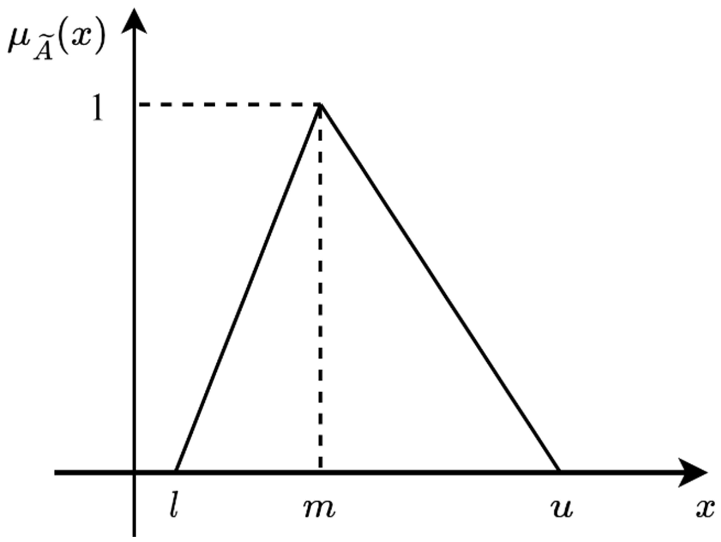
2.3. FST
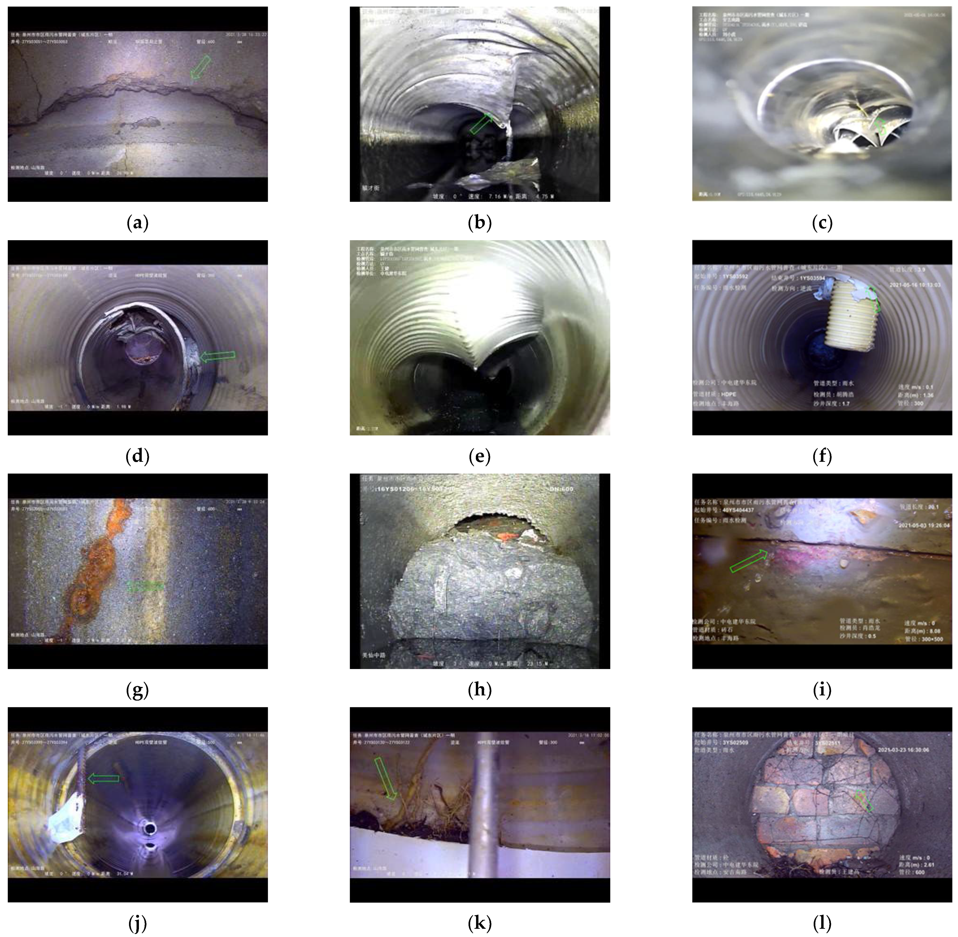
3. Failure Patterns of Drainage Pipes
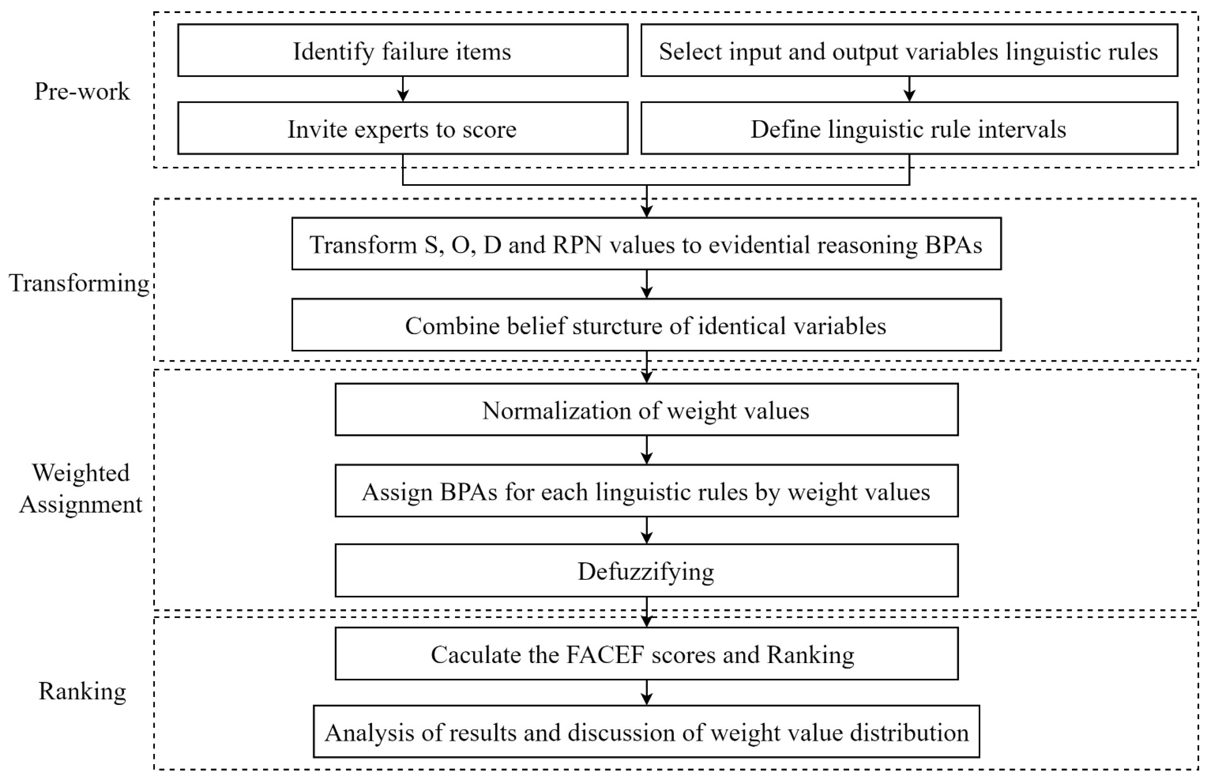
4. FMEA Approach by Using ER and FST
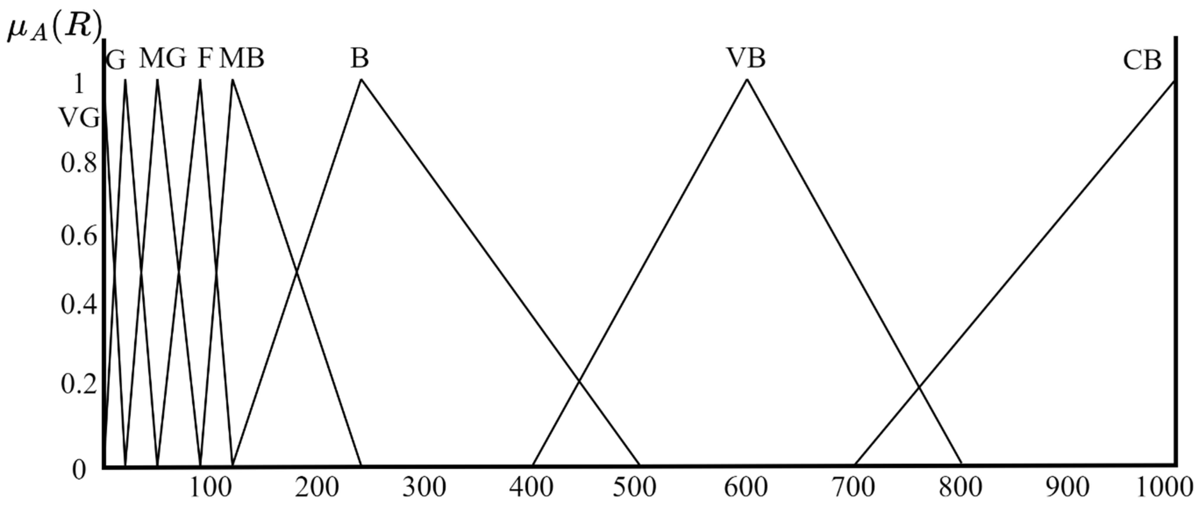
4.1. Defining Fuzzy Linguistic Rules
4.2. Transforming the Values of S, O, and D and RPNs to Evidential Reasoning BPAs
4.3. Constructing a Fuzzy Weighted ER Rule
4.3.1. Combining Same Rule Items
- Rule 1: IF , THEN
- Rule 2: IF , THEN
- Rule 3: IF , THEN
- Rule 4: IF , THEN
- Rule 5: IF , THEN
- Rule 6: IF , THEN
4.3.2. Belief Degree Assignment by Using Weight Values
4.4. Defuzzifying BPAs and Ranking
4.5. Chapter Discussion
5. Failure Risk Analysis by Using the Proposed Method
5.1. Pre-Work
- a)
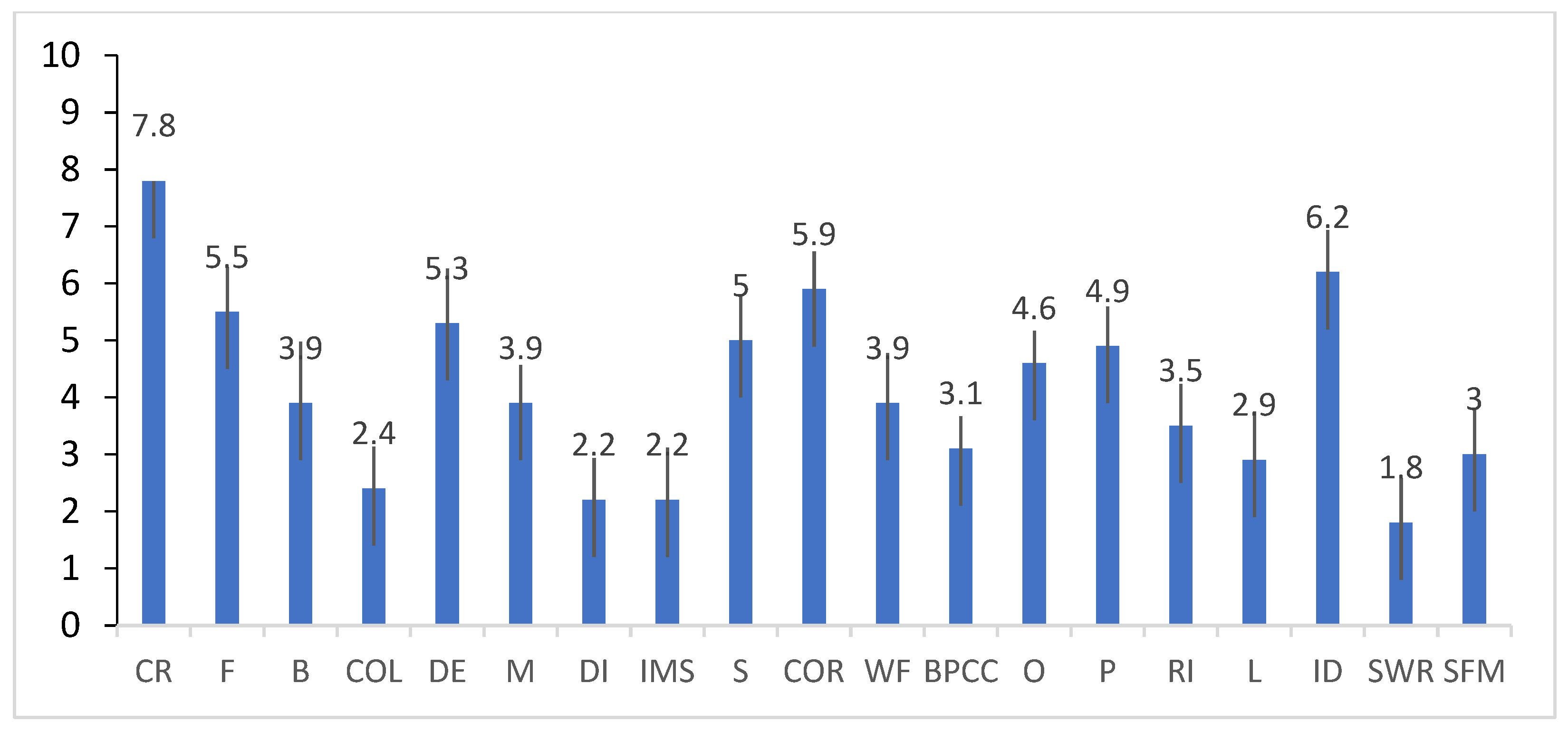
- From the distribution of extreme values in the S section, it can be seen that all experts consider collapse as a disaster with a great degree of damage, and half of the experts for broken also consider its damage impact to be great. Meanwhile, disconnect, branch pipe concealed connection, leakage, and stump walls and roots are considered by some experts to cause serious damage.
- b)
- In the O section, we have narrowed the range of extreme values selected, analyzing the reason may be that O in this study represents the probability of defect generation in the view of experts with an engineering background and scientific research background, resulting in a certain degree of quantitative loss (not generating a certain number of values greater than or equal to 9). In this extreme value interval, all the experts believe that the occurrence of cracks is very high, and the analysis may be due to the very high frequency of such failure in engineering practice. In addition, fracture, deformation, spalling, obstruction, penetration, and impurity deposits are considered high-frequency defects by experts in different degrees.
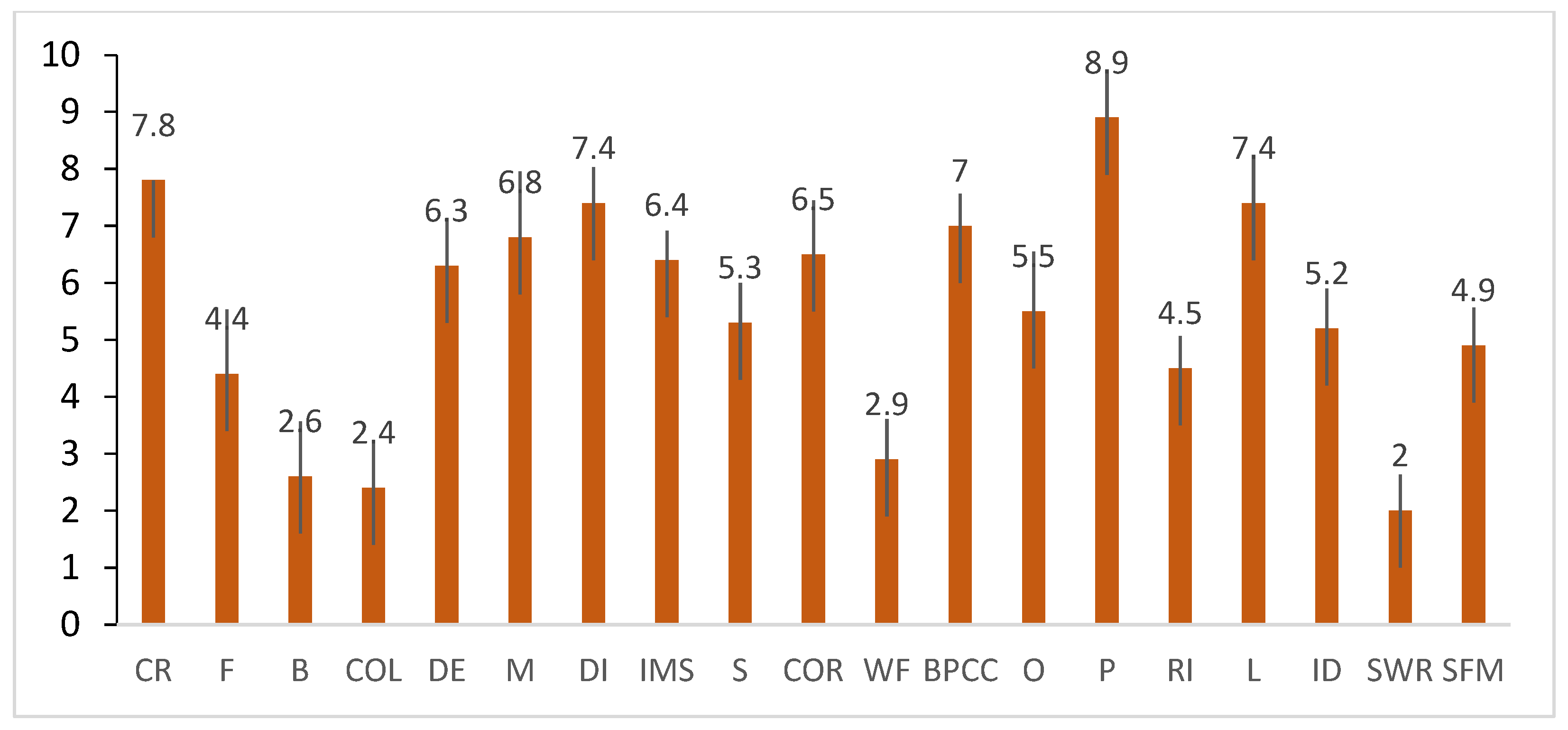
- c)
- As can be seen from the extreme value distribution of D in Table 8, penetration is considered to be the most difficult failure to be detected, probably due to the fact that the detection process mostly uses CCTV inspection, which requires pre-detection cleaning work, a process that greatly increases the difficulty of detecting penetration. Similarly, crack is also considered by experts to be the most difficult fault to be detected, presumably because the dim working environment inside the pipeline and the uncertainty of noise variables increase the difficulty of detection. In addition, deformation, mismatch, disconnect, corrosion, branch pipe concealed connection, and leakage have been identified by experts to varying degrees as difficult to detect failures.
5.2. Establishing a Fuzzy ER Rule on Sewer Pipeline Failures
6. Discussion
6.1. Result Analysis and Maintenance Measures
- a)
- Failures with FACEF scores ≥250: Penetration and crack are important failures that affect the condition of the pipeline, and as can be seen in Figure 7, Figure 8 and Figure 9, the S, O, and D scores for these two failures are at the high end of the scale, indicating that the severity of these failures is high, the probability of occurrence of these failures is relatively high, and that they are difficult to be detected. The clustered occurrence of penetration failure is attributed to inadequate planning of the surrounding environment during the pipeline design and construction phase, with a large number of complex foundation sections appearing in the vicinity of the pipeline, increasing the risk of pipeline penetration. Frequent changes in dynamic loads overlying the pipeline cause uneven stresses in the soil layer; this, in turn, accelerates the migration of foreign objects in the soil layer, posing a penetration risk to the outer wall of the pipeline. Some pipelines are made of soft materials that are easily penetrable (e.g., PVC) and have low internal resistance to penetration, making them more susceptible to penetration [25].
- b)
- Failures with FACEF scores ≥200: Deformation is a type of failure in which cross-sectional changes occur in the pipe structure under external extrusion. Due to aging, small-diameter flexural pipes become increasingly prone to deformation at the interfaces, and local soil builds up in the direction of the deformation, producing deformation over time. In flexural pipes such as HDPE, due to the lack of rigidity, existing unevenly stressed pipe wall local deformations get enlarged and gradually develop into cracks, severely affecting the structure of the pipe [42,43]. When uneven settlement of the overlying geotechnical body causes uneven external forces on the pipeline or when man-made construction causes damage to the pipeline, the pipeline structure changes, and deformation occurs [26]. Therefore, in the case of uneven soil cover around the pipeline or the presence of special soil, rigid pipelines with large diameter should be adopted to reduce the probability of deformation generation.
- c)
- Failures with FACEF scores ≥100: Common failures in this score range are corrosion and root intrusion. Corrosion is one of the most widely studied pipeline failures and is the main causative factor for most pipeline failures [41]. Corrosion is greatly affected by the pipe material; for example, concrete pipes [27] and galvanized copper pipes [52] are highly susceptible to corrosion. Seasonal changes also induce corrosion in pipes. Barton et al. concluded that the probability of corrosion in AC and PVC pipes is considerably higher in summer than in the other three seasons. Iron, ductile iron, and steel pipes are more prone to corrosion deterioration in the cold winter months than in the humid summer and mild autumn months [25]. The application of the pipeline is also an important factor contributing to corrosion. Ariaratnam et al. concluded that sewer pipes are the most prone to corrosion compared to stormwater pipes and combined sewage pipes [53]. Hahn et al. stated that biochemical, electrochemical, and physical reactions caused by the water inside the pipeline affect the long-term use of pipeline materials and highlighted that internal corrosion of the pipeline mainly depends on the nature of the liquid inside the pipeline [54]. To sum up, good protection of pipelines against corrosion and reasonable planning of pipeline route distribution can reduce the occurrence probability of corrosion in pipelines.
6.2. Algorithm Improvement and Discussion
- a)
- FACEF converts expert opinions into belief degrees for different output variable intervals, thus solving to some extent the problem that the approximate average values of RPNs obtained using TFMEA can cause ambiguity in experts’ perception of extreme values of evaluation and the belief degree can relatively objectively reflect experts’ perception, making the algorithm results more interpretative.
- b)
- TFMEA scores cannot be categorized due to excessive variations, making the secondary analysis of failures impossible. In contrast, FACEF scores can be categorized, thus enabling analyses highly relevant to engineering perceptions.
- c)
- FACEF results are greatly influenced by the belief degree and defuzzification values. Obtaining evaluation results from experts with different backgrounds is beneficial for obtaining information regarding different belief intervals and expanding the cognitive scope of the algorithm.
- d)
- The linguistic rule interval setting of FACEF can be understood as the total set of all cases that may have occurred or may occur in the future. As can be seen from Table 9, the frequency of two extreme cases, VB and CB, was extremely low; in particular, CB did not appear in the application of the evaluation model in this study, but the analysis results revealed that the RPN values required to reach these two extreme cases are extremely high (requiring to be assigned high values). Thus, these two extreme cases should be given special consideration. In the FACEF evaluation method, attention should be paid to the belief degrees assigned to these two groups of intervals, and if a failure has a belief degree of extreme cases, the reasons should be analyzed, and timely secondary evaluation and information feedback should be conducted to solve the problem.
7. Conclusions and Recommendations
- a)
- Five commonly used pipeline evaluation specification methods were analyzed, and 19 drainage pipeline failures were summarized by categorizing them into structural failures and operational failures.
- b)
- Ten experts with engineering or research backgrounds were consulted to assess the 19 pipe failures using expert opinion. Each failure was evaluated in terms of its severity (S), occurrence (O), and probability of being undetected (D). The results indicate that collapse, crack, and penetration had the highest scores in the S, O, and D sections, respectively.
- c)
- The newly developed algorithm was used to statistically process the expert scores, and the weight values for each failure were determined. The results reveal that penetration, crack, deformation, mismatch, leakage, and obstruction are the six pipeline failures that demand the most attention, and the S, O, and D weight distributions for typical failures in each scoring range are discussed in detail.
- a)
- The expert evaluation scoring revealed that only one score in the O section exceeded 8. This is primarily due to the fact that the score reflects the experts’ perception of the probability of a pipe failure (e.g., a score of nine corresponds to nearly 90% occurrence). Such situations should be avoided in future studies to minimize the potential loss of scores and increase the accuracy of the final results.
- b)
- Table 9 shows that the weights of the extreme intervals are minimal, making it difficult to perform further analysis on the weights. As a result, some of the advantages of the algorithm are lost. In future studies, the VB (Very High) and CB (Completely bad) intervals can be expanded to include a wider range of weights.
Author Contributions
Funding
Conflicts of Interest
Abbreviations
| B | Bad |
| BPA | Basic probability assignment |
| BPCC | Branch Pipe Concealed Connection |
| BR | Broken |
| CB | Completely bad |
| CCTV | Closed-circuit television |
| CIRCA | Conduit Inspection Reporting Code of Australia |
| CoG | Center of gravity |
| COL | Collapse |
| COR | Corrosion |
| CR | Crack |
| D | The probability of not detecting the failure |
| DE | Deformation |
| DI | Disconnect |
| ER | Evidential reasoning |
| F | Fair |
| FACEF | FMEA approach combined with ER and FST |
| FMEA | Failure mode and effect analysis |
| FR | Fracture |
| FST | Fuzzy set theory |
| G | Good |
| H | High |
| ID | Impurity Deposits |
| IMS | Interface Material Shedding |
| L | Low |
| LE | Leakage |
| MI | Mismatch |
| M | Middle |
| MB | Middle bad |
| MSCC | The manual of Sewer Condition Classification |
| O | The occurrence of failure mode |
| O&M | Operation and maintenance |
| OB | Obstruction |
| P | Penetration |
| PACP | Pipeline Assessment and Certification Program |
| PPT | Pignistic probability transformation |
| RI | Root Intrusion |
| RPN | Risk priority number |
| S | Severity of the failure |
| SP | Spalling |
| SFM | Scam and Floating Mud |
| SWR | Stump Walls and Roots |
| TFMEA | Traditional failure mode and effect analysis |
| TPN | Triangular fuzzy number |
| VB | Very bad |
| VG | Very good |
| VH | Very high |
| VL | Very low |
| WF | Weld Failure |
References
- Grengg, C.; Mittermayr, F.; Ukrainczyk, N.; Koraimann, G.; Kienesberger, S.; Dietzel, M. Advances in Concrete Materials for Sewer Systems Affected by Microbial Induced Concrete Corrosion: A Review. Water Res. 2018, 134, 341–352. [Google Scholar] [CrossRef] [PubMed]
- Wang, J.; Liu, G.; Wang, J.; Xu, X.; Shao, Y.; Zhang, Q.; Liu, Y.; Qi, L.; Wang, H. Current Status, Existent Problems, and Coping Strategy of Urban Drainage Pipeline Network in China. Environ. Sci. Pollut. Res. 2021, 28, 43035–43049. [Google Scholar] [CrossRef] [PubMed]
- Li, Y.; Wang, W.; He, M.; Shen, T. Mechanism of urban black odorous based on continuous monitoring: A case study of the Erkeng stream in Nanning. Environ. Sci. 2020, 41, 2257–2263. [Google Scholar] [CrossRef]
- Rahmawati, R.; Firman, F. The Politics of Clean Water Management: A Critical Review on the Scarcity of Clean Water in Kedungringin Village. ARISTO 2022, 11, 114–125. [Google Scholar] [CrossRef]
- Sakai, H.; Satake, M.; Arai, Y.; Takizawa, S. Report Cards for Aging and Maintenance Assessment of Water-Supply Infrastructure. J. Water Supply Res. Technol.-Aqua 2020, 69, 355–364. [Google Scholar] [CrossRef] [Green Version]
- Huang, D.; Liu, X.; Jiang, S.; Wang, H.; Wang, J.; Zhang, Y. Current State and Future Perspectives of Sewer Networks in Urban China. Front. Environ. Sci. Eng. 2018, 12, 2. [Google Scholar] [CrossRef]
- Belogurov, V.; Fafurdinova, G. GIS-Technology of Water Drainage System (WDS) Modernization in Ukrainian City with Rugged Terrain. Int. J. 2022, 11, 6. [Google Scholar]
- Dastgir, A.; Hesarkazzazi, S.; Oberascher, M.; Hajibabaei, M.; Sitzenfrei, R. Graph Method for Critical Pipe Analysis of Branched and Looped Drainage Networks. Water Sci. Technol. 2023, 87, 157–173. [Google Scholar] [CrossRef]
- Kuliczkowska, E. Risk of Structural Failure in Concrete Sewers Due to Internal Corrosion. Eng. Fail. Anal. 2016, 66, 110–119. [Google Scholar] [CrossRef]
- Paternina-Verona, D.A.; Coronado-Hernández, O.E.; Espinoza-Román, H.G.; Besharat, M.; Fuertes-Miquel, V.S.; Ramos, H.M. Three-Dimensional Analysis of Air-Admission Orifices in Pipelines during Hydraulic Drainage Events. Sustainability 2022, 14, 14600. [Google Scholar] [CrossRef]
- Mohamed, M.A.-H.; Ramadan, M.A.; El-Dash, K.M. Cost Optimization of Sewage Pipelines Inspection. Ain Shams Eng. J. 2023, 14, 101960. [Google Scholar] [CrossRef]
- Salihu, C.; Hussein, M.; Mohandes, S.R.; Zayed, T. Towards a Comprehensive Review of the Deterioration Factors and Modeling for Sewer Pipelines: A Hybrid of Bibliometric, Scientometric, and Meta-Analysis Approach. J. Clean. Prod. 2022, 351, 131460. [Google Scholar] [CrossRef]
- Peeters, J.F.W.; Basten, R.J.; Tinga, T. Improving Failure Analysis Efficiency by Combining FTA and FMEA in a Recursive Manner. Reliab. Eng. Syst. Saf. 2018, 172, 36–44. [Google Scholar] [CrossRef] [Green Version]
- Bozdag, E.; Asan, U.; Soyer, A.; Serdarasan, S. Risk Prioritization in Failure Mode and Effects Analysis Using Interval Type-2 Fuzzy Sets. Expert Syst. Appl. 2015, 42, 4000–4015. [Google Scholar] [CrossRef]
- Wu, Z.; Liu, W.; Nie, W.; Wu, Z.; Liu, W.; Nie, W. Literature Review and Prospect of the Development and Application of FMEA in Manufacturing Industry. Int. J. Adv. Manuf. Technol. 2021, 112, 1409–1436. [Google Scholar] [CrossRef]
- Rastayesh, S.; Bahrebar, S.; Blaabjerg, F.; Zhou, D.; Wang, H.; Dalsgaard Sørensen, J. A System Engineering Approach Using FMEA and Bayesian Network for Risk Analysis—A Case Study. Sustainability 2020, 12, 77. [Google Scholar] [CrossRef] [Green Version]
- Liu, H.-C.; Liu, L.; Liu, N. Risk Evaluation Approaches in Failure Mode and Effects Analysis: A Literature Review. Expert Syst. Appl. 2013, 40, 828–838. [Google Scholar] [CrossRef]
- Dempster, A.P. Upper and Lower Probabilities Induced by a Multivalued Mapping. Ann. Math. Stat. 1967, 38, 325–339. [Google Scholar] [CrossRef]
- Shafer, G. A Mathematical Theory of Evidence; Princeton University Press: Princeton, NJ, USA, 1976; ISBN 978-0-691-10042-5. [Google Scholar]
- Limboo, B.; Dutta, P. A Q-Rung Orthopair Basic Probability Assignment and Its Application in Medical Diagnosis. Decis. Mak. Appl. Manag. Eng. 2022, 5, 290–308. [Google Scholar] [CrossRef]
- Zhang, T. Research on Evaluation of Supported High and Steep Loess Slope Based on D-S Evidential Reasoning. Master’s Thesis, Chang’an University, Xi’an, China, 2019. [Google Scholar]
- Smets, P. The Transferable Belief Model. Artif. Intell. 1994, 66, 191–234. [Google Scholar] [CrossRef]
- Deng, X.; Jiang, W. D Number Theory Based Game-Theoretic Framework in Adversarial Decision Making under a Fuzzy Environment. Int. J. Approx. Reason. 2019, 106, 194–213. [Google Scholar] [CrossRef]
- Akyar, E.; Akyar, H.; Düzce, S.A. A new method for ranking triangular fuzzy numbers. Int. J. Unc. Fuzz. Knowl. Based Syst. 2012, 20, 729–740. [Google Scholar] [CrossRef]
- Barton, N.A.; Farewell, T.S.; Hallett, S.H.; Acland, T.F. Improving Pipe Failure Predictions: Factors Affecting Pipe Failure in Drinking Water Networks. Water Res. 2019, 164, 114926. [Google Scholar] [CrossRef] [PubMed]
- Davies, J.P.; Clarke, B.A.; Whiter, J.T.; Cunningham, R.J. Factors Influencing the Structural Deterioration and Collapse of Rigid Sewer Pipes. Urban Water 2001, 17, 73–89. [Google Scholar] [CrossRef]
- Malek Mohammadi, M.; Najafi, M.; Kermanshachi, S.; Kaushal, V.; Serajiantehrani, R. Factors Influencing the Condition of Sewer Pipes: State-of-the-Art Review. J. Pipeline Syst. Eng. Pract. 2020, 11, 03120002. [Google Scholar] [CrossRef]
- Liu, Z.; Kleiner, Y. State of the Art Review of Inspection Technologies for Condition Assessment of Water Pipes. Measurement 2013, 46, 1–15. [Google Scholar] [CrossRef] [Green Version]
- Zuo, X.; Dai, B.; Shan, Y.; Shen, J.; Hu, C.; Huang, S. Classifying Cracks at Sub-Class Level in Closed Circuit Television Sewer Inspection Videos. Autom. Constr. 2020, 118, 103289. [Google Scholar] [CrossRef]
- Li, D.; Xie, Q.; Yu, Z.; Wu, Q.; Zhou, J.; Wang, J. Sewer Pipe Defect Detection via Deep Learning with Local and Global Feature Fusion. Autom. Constr. 2021, 129, 103823. [Google Scholar] [CrossRef]
- Water Research Centre. Sewerage Rehabilitation Manual; WRc Publ: Wiltshire, UK, 2001; ISBN 978-1-898920-39-7. [Google Scholar]
- National Association of Sewer Service Companies. Pipeline Assessment Certification Manual; National Association of Sewer Service Companies: Marriottsville, MD, USA, 2018. [Google Scholar]
- Water Services Association of Australia. Conduit Inspection Reporting Code of Australia, 4th ed.; Water Services Association of Australia: Melbourne, Australia, 2020. [Google Scholar]
- Jiang, W.; Zhang, Z.; Deng, X. A Novel Failure Mode and Effects Analysis Method Based on Fuzzy Evidential Reasoning Rules. IEEE Access 2019, 7, 113605–113615. [Google Scholar] [CrossRef]
- Cheng, M.; Lu, Y. Developing a Risk Assessment Method for Complex Pipe Jacking Construction Projects. Autom. Constr. 2015, 58, 48–59. [Google Scholar] [CrossRef]
- Kadena, E.; Koçak, S.; Takács-György, K.; Keszthelyi, A. FMEA in Smartphones: A Fuzzy Approach. Mathematics 2022, 10, 513. [Google Scholar] [CrossRef]
- Yahaya, N.Y.N.; Lim, K.L.K.; Noor, N.N.N.; Othman, S.O.S.; Abdullah, A.A.A. Effects of Clay and Moisture Content on Soil-Corrosion Dynamic. Malays. J. Civ. Eng. 2011, 23, 24–32. [Google Scholar] [CrossRef]
- Pritchard, O.; Hallett, S.H.; Farewell, T.S. Soil Corrosivity in the UK–Impacts on Critical Infrastructure; ITRC–Infrastructure Transition Research Consortium, Cranfield University: Cranfield, UK, 2013. [Google Scholar]
- Liao, B.; Ti, Z.; Ma, B. Analysis of the causes of collapse of large diameter buried HDPE drainage pipes and non-excavation repair measures introduced. Water Wastewater 2015, 51, 75–77. [Google Scholar] [CrossRef]
- Salman, B. Infrastructure Management and Deterioration Risk Assessment of Wastewater Collection Systems; University of Cincinnati: Cincinnati, OH, USA, 2010; ISBN 1-124-35964-8. [Google Scholar]
- Steven, F. Water Main Break Rates in the USA and Canada: A Comprehensive Study; Utah State University: Logan, UT, USA, 2018; Volume 48. [Google Scholar]
- Kimutai, E.; Betrie, G.; Brander, R.; Sadiq, R.; Tesfamariam, S. Comparison of Statistical Models for Predicting Pipe Failures: Illustrative Example with the City of Calgary Water Main Failure. J. Pipeline Syst. Eng. Pract. 2015, 6, 04015005. [Google Scholar] [CrossRef]
- Bruaset, S.; Sægrov, S. An Analysis of the Potential Impact of Climate Change on the Structural Reliability of Drinking Water Pipes in Cold Climate Regions. Water 2018, 10, 411. [Google Scholar] [CrossRef] [Green Version]
- Lu, S. Design and Performance of Cement Mortar for Connection of Reinforced Concrete Drainage Pipeline. Master’s Thesis, University of South China, Hengyang, China, 2020. [Google Scholar]
- Meijering, T.G.; Wolters, M.; Hermkens, R.J. The Durability of a Low-Pressure Gas Distribution System of Ductile PVC. In Proceedings of the 12th International Conference on Plastics Pipes, Milan, Italy, 19–22 April 2004. [Google Scholar]
- Zamanian, S.; Hur, J.; Shafieezadeh, A. Significant Variables for Leakage and Collapse of Buried Concrete Sewer Pipes: A Global Sensitivity Analysis via Bayesian Additive Regression Trees and Sobol’indices. Struct. Infrastruct. Eng. 2021, 17, 676–688. [Google Scholar] [CrossRef]
- Lai, W.L.; Kou, S.C.; Poon, C.S. Unsaturated Zone Characterization in Soil through Transient Wetting and Drying Using GPR Joint Time–Frequency Analysis and Grayscale Images. J. Hydrol. 2012, 452–453, 1–13. [Google Scholar] [CrossRef]
- Ran, Q. Numerical Simulation and Acoustic Location of Water Supply Pipeline Leakage. Master’s Thesis, Beijing University of Civil Engineering and Architecture, Beijing, China, 2021. [Google Scholar]
- Li, S.; Song, Y.; Zhou, G. Leak Detection of Water Distribution Pipeline Subject to Failure of Socket Joint Based on Acoustic Emission and Pattern Recognition. Measurement 2018, 115, 39–44. [Google Scholar] [CrossRef]
- Zaman, D.; Tiwari, M.K.; Gupta, A.K.; Sen, D. A Review of Leakage Detection Strategies for Pressurised Pipeline in Steady-State. Eng. Fail. Anal. 2020, 109, 104264. [Google Scholar] [CrossRef]
- Fan, H.; Tariq, S.; Zayed, T. Acoustic Leak Detection Approaches for Water Pipelines. Autom. Constr. 2022, 138, 104226. [Google Scholar] [CrossRef]
- Zhou, C.; Yang, L.; Zhang, Y.; Zhang, J.; Gao, L.; Duan, R.; Wu, M.; Zhao, X. Application of grey correlation analysis in evaluation of leakage factors in water supply network of a city in North China. Water Wastewater 2019, 55, 123–127+139. [Google Scholar] [CrossRef]
- Ariaratnam, S.T.; El-Assaly, A.; Yang, Y. Assessment of Infrastructure Inspection Needs Using Logistic Models. J. Infrastruct. Syst. 2001, 7, 160–165. [Google Scholar] [CrossRef]
- Hahn, M.A.; Palmer, R.N.; Merrill, M.S.; Lukas, A.B. Expert System for Prioritizing the Inspection of Sewers: Knowledge Base Formulation and Evaluation. J. Water Resour. Plann. Manag. 2002, 128, 121–129. [Google Scholar] [CrossRef] [Green Version]
- Orvesten, A.; Stål, Ö. Trädrötter Och Ledningar-Goda Exempel På Lösningar Och Samarbetsformer. Sven. Vatten Och Avloppsverksföreningen. VA-FORSK Rep. 2003, 31, 2003. [Google Scholar]
- Ridgers, D.; Rolf, K.; Stål, Ö. Management and Planning Solutions to Lack of Resistance to Root Penetration by Modern Pvc and Concrete Sewer Pipes. Arboric. J. 2006, 29, 269–290. [Google Scholar] [CrossRef]
- Li, R. A Study of Urban Sewer Inspection, Assessment and Related Factors. Master’s Thesis, Tsinghua University, Beijing, China, 2016. [Google Scholar]


| Failure Name | Description | |
|---|---|---|
| Structural Failures | Crack (CR) | The outer wall of the pipe produces obvious crack lines, but no obvious breakage of the pipe wall occurs |
| Fracture (FR) | Cracks in the outer wall of the pipe are clearly cracked, but the broken pieces of pipe are still in place | |
| Broken (BR) | Some parts of the pipe are clearly separated, and the lost parts are no longer in place | |
| Collapse (COL) | The whole cross-section of the pipe is disconnected and cannot form an effective water interception section | |
| Deformation (DE) | There is a significant cross-sectional change in one part of the pipe compared to the nearby area | |
| Mismatch (MI) | The two orifices of the same interface produce lateral deviation and are not in the correct position of the pipe | |
| Disconnect (DI) | The ends of the two pipes are not sufficiently joined, or the interfaces are detached | |
| Interface Material Shedding (IMS) | Rubber ring, asphalt, cement, and other similar interface materials into the pipe | |
| Spalling (SP) | Pipe surface material breaks into small pieces due to corrosion of reinforcement or expansion of poor-quality material | |
| Corrosion (COR) | The inner wall of the pipe is eroded and lost or spalled, appearing pockmarked or exposed steel | |
| Weld Failure (WF) | Interface damage caused by improper human operation or material deformation at the pipeline interface during welding | |
| Branch Pipe Concealed Connection (BPCC) | The branch pipe is not directly connected to the main lateral through the inspection well | |
| Operational Failures | Obstruction (OB) | There are obstructions inside the pipe that affect the overflow of the pipe |
| Penetration (P) | Insertion of external objects other than the pipe itself or appurtenances into the pipe | |
| Root Intrusion (RI) | Individual roots or scaled roots grow naturally into the pipe | |
| Leakage (LE) | Water infiltration or seepage caused by structural damage to the pipe itself | |
| Impurity Deposits (ID) | Sedimentation and siltation of impurities at the bottom of the pipe | |
| Stump Walls and Roots (SWR) | Temporary brick wall blocking masonry when the pipe closed water test after the test is not removed or removed incomplete | |
| Scam and Floating Mud (SFM) | There is a collection of floating objects on the water surface in the pipe |
| Linguistic Level | TPN | |||
|---|---|---|---|---|
| VL | (0, 0, 2.5) | Minimal impact on pipeline management | Very low probability of occurrence | Very easy to detect |
| L | (0, 2.5, 5) | Low impact on pipeline management | Low probability of occurrence | Easy to detect |
| M | (2.5, 5, 7.5) | Insignificant impact on pipeline management | Moderate probability of occurrence | Moderate probability of detection |
| H | (5, 7.5, 10) | High impact on pipeline management | High probability of occurrence | Hard to detect |
| VH | (7.5, 10, 10) | Great impact on pipeline management | Very high probability of occurrence | Almost undetectable |
| Linguistic Level | VG | G | MG | F | MB | B | VB | CB |
|---|---|---|---|---|---|---|---|---|
| Range | (0, 0, 20) | (0, 20, 60) | (20, 60, 90) | (60, 90, 120) | (90, 120, 240) | (120, 240, 500) | (400, 600, 800) | (700, 1000, 1000) |
| Rule | S | O | D | RPN |
|---|---|---|---|---|
| Rule 5 | ||||
| Rule 6 | ||||
| Rule 7 | ||||
| Rule 8 |
| Rule | S | O | D | RPN |
|---|---|---|---|---|
| Rule 1 | ||||
| Rule 2 | ||||
| Rule 3 | ||||
| Rule 4 |
| Rules | S | O | D | Before Combined BPAs | Combined BPAs |
|---|---|---|---|---|---|
| Rule 1, Rule 5 | |||||
| Rule 3, Rule 7 |
| Linguistic Item | VG | G | MG | F | MB | B | VB | CB |
|---|---|---|---|---|---|---|---|---|
| CoG | 6.6667 | 26.6667 | 56.6667 | 90 | 150 | 286.6667 | 600 | 900 |
| CR | FR | BR | COL | DE | MI | DI | IMS | SP | COR | WF | BPCC | OB | P | RI | LE | ID | SWR | SFM | |
|---|---|---|---|---|---|---|---|---|---|---|---|---|---|---|---|---|---|---|---|
| S | 5 | 7 | 9 | 10 | 6 | 7 | 8 | 3 | 2 | 2 | 5 | 7 | 8 | 7 | 8 | 8 | 5 | 9 | 2 |
| 5 | 7 | 8 | 9 | 5 | 8 | 8 | 3 | 3 | 4 | 5 | 8 | 7 | 8 | 7 | 9 | 6 | 8 | 2 | |
| 6 | 8 | 9 | 10 | 6 | 8 | 9 | 2 | 2 | 3 | 4 | 7 | 7 | 6 | 7 | 8 | 5 | 9 | 3 | |
| 6 | 8 | 8 | 9 | 6 | 7 | 8 | 4 | 3 | 3 | 6 | 8 | 8 | 7 | 8 | 8 | 5 | 8 | 2 | |
| 5 | 7 | 9 | 10 | 5 | 8 | 9 | 3 | 3 | 3 | 5 | 7 | 7 | 8 | 8 | 10 | 4 | 8 | 2 | |
| 4 | 7 | 10 | 9 | 7 | 7 | 7 | 3 | 4 | 5 | 5 | 8 | 8 | 7 | 7 | 8 | 5 | 8 | 2 | |
| 5 | 7 | 8 | 10 | 6 | 7 | 8 | 3 | 3 | 4 | 6 | 9 | 8 | 7 | 8 | 8 | 5 | 9 | 1 | |
| 6 | 6 | 9 | 10 | 6 | 8 | 8 | 2 | 3 | 4 | 5 | 7 | 7 | 7 | 7 | 8 | 4 | 8 | 2 | |
| 4 | 8 | 8 | 10 | 5 | 7 | 7 | 3 | 3 | 2 | 5 | 9 | 7 | 8 | 7 | 9 | 6 | 7 | 3 | |
| 5 | 7 | 8 | 10 | 7 | 7 | 8 | 3 | 3 | 3 | 5 | 8 | 8 | 7 | 8 | 9 | 5 | 8 | 2 | |
| O | 7 | 6 | 3 | 3 | 5 | 4 | 4 | 1 | 5 | 7 | 4 | 2 | 4 | 5 | 5 | 4 | 6 | 1 | 2 |
| 7 | 5 | 5 | 2 | 5 | 4 | 2 | 2 | 6 | 5 | 4 | 3 | 4 | 4 | 4 | 3 | 6 | 1 | 3 | |
| 8 | 7 | 4 | 3 | 6 | 3 | 2 | 2 | 5 | 6 | 3 | 3 | 5 | 4 | 4 | 4 | 7 | 2 | 4 | |
| 7 | 6 | 3 | 1 | 4 | 5 | 3 | 3 | 4 | 7 | 5 | 4 | 6 | 6 | 3 | 2 | 7 | 2 | 3 | |
| 8 | 5 | 4 | 4 | 6 | 4 | 1 | 3 | 5 | 6 | 4 | 3 | 4 | 5 | 4 | 2 | 5 | 1 | 3 | |
| 9 | 7 | 4 | 2 | 5 | 5 | 2 | 3 | 5 | 7 | 3 | 3 | 5 | 5 | 4 | 3 | 7 | 3 | 2 | |
| 8 | 4 | 5 | 1 | 5 | 3 | 2 | 2 | 6 | 5 | 4 | 3 | 5 | 5 | 3 | 3 | 6 | 2 | 3 | |
| 8 | 5 | 3 | 3 | 6 | 4 | 2 | 1 | 4 | 5 | 4 | 3 | 4 | 5 | 2 | 3 | 5 | 2 | 5 | |
| 9 | 6 | 4 | 2 | 6 | 3 | 3 | 3 | 5 | 6 | 4 | 4 | 4 | 6 | 3 | 3 | 6 | 1 | 2 | |
| 7 | 4 | 4 | 3 | 5 | 4 | 1 | 2 | 5 | 5 | 4 | 3 | 5 | 4 | 3 | 2 | 7 | 3 | 3 | |
| D | 9 | 5 | 3 | 3 | 8 | 6 | 8 | 6 | 4 | 6 | 3 | 6 | 7 | 9 | 5 | 7 | 5 | 2 | 6 |
| 9 | 6 | 2 | 1 | 7 | 7 | 7 | 7 | 5 | 6 | 3 | 7 | 6 | 9 | 6 | 8 | 6 | 3 | 5 | |
| 6 | 4 | 4 | 2 | 5 | 7 | 7 | 7 | 4 | 7 | 4 | 7 | 5 | 8 | 4 | 7 | 5 | 1 | 4 | |
| 8 | 5 | 2 | 3 | 8 | 8 | 7 | 6 | 5 | 8 | 3 | 6 | 6 | 8 | 5 | 6 | 5 | 2 | 4 | |
| 9 | 4 | 3 | 2 | 6 | 7 | 7 | 7 | 6 | 6 | 3 | 8 | 5 | 9 | 4 | 7 | 4 | 2 | 6 | |
| 8 | 5 | 3 | 2 | 5 | 6 | 8 | 6 | 5 | 6 | 2 | 6 | 5 | 9 | 5 | 8 | 5 | 3 | 5 | |
| 6 | 5 | 1 | 3 | 6 | 7 | 8 | 5 | 5 | 7 | 3 | 7 | 6 | 10 | 4 | 8 | 6 | 2 | 5 | |
| 7 | 4 | 2 | 4 | 7 | 6 | 7 | 7 | 7 | 6 | 3 | 9 | 4 | 9 | 5 | 7 | 5 | 1 | 3 | |
| 8 | 3 | 3 | 2 | 6 | 7 | 7 | 6 | 6 | 6 | 2 | 6 | 6 | 9 | 4 | 8 | 5 | 2 | 5 | |
| 8 | 3 | 3 | 2 | 5 | 7 | 8 | 7 | 6 | 7 | 3 | 8 | 5 | 9 | 3 | 8 | 6 | 2 | 6 |
| VG | G | MG | F | MB | B | VB | CB | |
|---|---|---|---|---|---|---|---|---|
| CR | 0 | 0 | 0 | 0 | 0 | 1 | 0 | 0 |
| FR | 0 | 0 | 0.02004 | 0.18036 | 0.38231 | 0.41728 | 0 | 0 |
| BR | 0 | 0.38102 | 0.27704 | 0.33162 | 0.34573 | 0.00752 | 0 | 0 |
| COL | 0.00718 | 0.35239 | 0.23920 | 0.32226 | 0.07889 | 0 | 0 | 0 |
| DE | 0 | 0 | 0 | 0 | 0.34259 | 0.65741 | 0 | 0 |
| MI | 0 | 0 | 0 | 0 | 0.49678 | 0.50322 | 0 | 0 |
| DI | 0 | 0 | 0.24661 | 0.07233 | 0.56447 | 0.11659 | 0 | 0 |
| IMS | 0.05725 | 0.39471 | 0.46742 | 0.08063 | 0 | 0 | 0 | 0 |
| SP | 0 | 0.05908 | 0.32831 | 0.59737 | 0.01524 | 0 | 0 | 0 |
| COR | 0 | 0 | 0.17902 | 0.25993 | 0.47840 | 0.08266 | 0 | 0 |
| WF | 0 | 0.21036 | 0.37947 | 0.41017 | 0 | 0 | 0 | 0 |
| BPCC | 0 | 0 | 0.01188 | 0.10690 | 0.47568 | 0.40554 | 0 | 0 |
| OB | 0 | 0 | 0 | 0.04816 | 0.49211 | 0.45973 | 0 | 0 |
| P | 0 | 0 | 0 | 0 | 0.02269 | 0.96395 | 0.01337 | 0 |
| RI | 0 | 0 | 0.14304 | 0.32324 | 0.47456 | 0.05916 | 0 | 0 |
| LE | 0 | 0 | 0 | 0.06966 | 0.41288 | 0.51747 | 0 | 0 |
| ID | 0 | 0 | 0.02799 | 0.16284 | 0.36584 | 0.44334 | 0 | 0 |
| SWR | 0.03989 | 0.58861 | 0.33426 | 0.03724 | 0 | 0 | 0 | 0 |
| SFM | 0.02764 | 0.74026 | 0.23211 | 0 | 0 | 0 | 0 | 0 |
| Failure | FACEF | Ranking of FACEF | Traditional FMEA | Ranking of TFMEA |
|---|---|---|---|---|
| Penetration | 287.7597 | 1 | 315.5 | 1 |
| Crack | 286.6667 | 2 | 304.6 | 2 |
| Deformation | 239.8461 | 3 | 192.9 | 4 |
| Mismatch | 218.7734 | 4 | 195.6 | 3 |
| Leakage | 216.5428 | 5 | 181.2 | 6 |
| Obstruction | 209.9402 | 6 | 191.5 | 5 |
| Impurity Deposits | 198.2085 | 7 | 164.4 | 9 |
| Branch Pipe Concealed Connection | 197.901 | 8 | 168.9 | 8 |
| Fracture | 194.3348 | 9 | 175.7 | 7 |
| Disconnect | 138.5772 | 10 | 128.8 | 10 |
| Corrosion | 128.994 | 11 | 125.3 | 11 |
| Root Intrusion | 125.3404 | 12 | 119 | 12 |
| Broken | 109.7205 | 13 | 86.7 | 13 |
| Spalling | 76.22901 | 14 | 77.4 | 14 |
| Weld Failure | 64.02822 | 15 | 58 | 15 |
| Collapse | 63.8365 | 16 | 56.1 | 16 |
| Interface Material Shedding | 44.65113 | 17 | 41.7 | 17 |
| Stump Walls and Roots | 38.25523 | 18 | 29.4 | 18 |
| Scam and Floating Mud | 33.07747 | 19 | 29.3 | 19 |
Disclaimer/Publisher’s Note: The statements, opinions and data contained in all publications are solely those of the individual author(s) and contributor(s) and not of MDPI and/or the editor(s). MDPI and/or the editor(s) disclaim responsibility for any injury to people or property resulting from any ideas, methods, instructions or products referred to in the content. |
© 2023 by the authors. Licensee MDPI, Basel, Switzerland. This article is an open access article distributed under the terms and conditions of the Creative Commons Attribution (CC BY) license (https://creativecommons.org/licenses/by/4.0/).
Share and Cite
Wang, Z.; Yang, Y.; Wang, H.; Zeng, X. A Comprehensive Failure Risk Analysis of Drainage Pipes Utilizing Fuzzy Failure Mode and Effect Analysis and Evidential Reasoning. Buildings 2023, 13, 590. https://doi.org/10.3390/buildings13030590
Wang Z, Yang Y, Wang H, Zeng X. A Comprehensive Failure Risk Analysis of Drainage Pipes Utilizing Fuzzy Failure Mode and Effect Analysis and Evidential Reasoning. Buildings. 2023; 13(3):590. https://doi.org/10.3390/buildings13030590
Chicago/Turabian StyleWang, Zinan, Yuxuan Yang, Hao Wang, and Xuming Zeng. 2023. "A Comprehensive Failure Risk Analysis of Drainage Pipes Utilizing Fuzzy Failure Mode and Effect Analysis and Evidential Reasoning" Buildings 13, no. 3: 590. https://doi.org/10.3390/buildings13030590