Modelling Strategies for the Updating of Infilled RC Building FEMs Considering the Construction Phases

Abstract

This paper deals with modelling strategies for the updating of Finite Element Models (FEMs) of infilled Reinforced Concrete (RC) frame buildings. As is known, this building typology is the most adopted worldwide for residential houses and strategic buildings, such as hospitals, schools, police stations, etc. The importance of achieving trustworthy numerical models for these kinds of structures, especially the latter ones, is clear. The updating procedure mainly consists in changing the geometrical and mechanical material properties of models until pre-determined convergence criteria are verified, the latter based on the comparison between numerical and experimental outcomes. In this work, the modelling strategies that can be adopted to refine FEMs of infilled RC buildings are treated in-depth, starting from the simple model usually developed for design purposes. Modelling techniques relevant to the geometry, the mechanical properties, the mass, and the restraint conditions of the model are discussed. Moreover, the approaches that can be adopted to calibrate numerical models during the construction process are addressed as well. Then, an application of the proposed strategies is provided with reference to a real building that was investigated during its construction. The proposed modelling strategies proved to be effective in the model updating of the considered building and provide useful support for the calibration of FEMs of this building typology in general.

1. Introduction

Despite the availability of extremely advanced and contemporary finite element methodologies for structural analysis, real applications frequently denote a sizable gap between analytical predictions and test findings [1]. Modifying the modelling assumptions and parameters until the connection between analytical results and experimental findings is not a simple task. The process that tries to solve this issue is called model updating, which essentially consists of adjusting some parts of the Finite Element Model (FEM) until the convergence between numerical and experimental outcomes, the latter measured on the considered structure [2,3,4,5]. Classically, this procedure is performed by adopting trial-and-error approaches, which are usually time consuming and sometimes may not be feasible [6]. Often, the model updating may be performed by refining the FEM in a known manner, trying to simulate the real properties of the structure (geometry, material mechanical properties, etc.) [7]. More recently, artificial intelligence algorithms have also been developed, trying to provide support on this topic [8,9]. For example, Ierimonti et al. [10], Akhlangji et al. [11], and Lam et al. [12] investigated the effectiveness of Bayesian model updating methods and their contribution within the framework of the model updating automatization. In addition, Rosati et al. [13] studied the usefulness of the Douglas−Reid model updating methods. These methodologies have the great advantage of reducing the updating process time; nevertheless, their use is not free from concerns since the achieved solution cannot always be representative of reality. For this reason, Boscato et al. [14] underline the importance of developing a preliminary sensitivity analysis that permits us to understand which parameters mostly affect the model behaviour and, most of all, to define plausible ranges of variation for the parameters considered in the updating procedure. In the civil engineering field, the model updating technique can be used to calibrate FEMs of buildings and infrastructures that can be useful for many purposes [15]. For instance, in their work, Pan et al. [16] discussed the importance of updating the model of a tall building located in Shanghai for the subsequent investigation of its seismic behaviour. Gentile and Saisi [17] applied the model updating methods to calibrate the numerical model of a historical tower. Foti et al. [18] and Astroza and Alessandri [19] adopted the model updating technique to calibrate numerical models of buildings also considering the presence of damage due to earthquakes. This is extremely important when the remaining useful life of a structure struck by a seismic sequence should be determined to avoid endangering people’s lives and unnecessary evacuations. The very recent earthquakes in Turkey [20], which caused an enormous number of victims, proved that buildings damaged by the main shake might collapse during aftershocks due to the accumulation of seismic damage. Moreover, in the case of infilled Reinforced Concrete (RC) buildings, the model updating technique also allows the aspects of the nonstructural element modelling to be addressed [21,22,23].

Updated models can support the design of SHM systems by implementing numerical studies that enable the identification of the right number and location of sensors in order to identify as many vibration modes as necessary (for instance, adopting optimal sensor placement procedures [24,25,26]). In addition, they may be used to numerically examine plausible damage scenarios in which structural member damage (and sometimes even failure), as well as environmentally catastrophic consequences (floods, landslides, pier scours, etc.), are taken into account, and their implications on the performance of the structure are explored [27,28,29]. Additionally, modifications to the dynamic behaviour are examined during these damage simulations in order to reach thresholds that may be included in dynamic monitoring systems for the SHM of buildings [30,31,32]. These numerical simulations are of paramount importance for supporting the management of the monitoring and maintenance activities. Moreover, a calibrated FEM is the first step for obtaining a digital twin of the construction [33,34]. This represents a milestone in the digitalization of the structure management process, with the main aim of gaining new frontiers in the field of construction engineering, namely the development of the so-called smart buildings [35].

The updating of FEMs may also be used as a technique for controlling the activities during the construction process of a building [36,37,38]. For example, a step-by-step FEM of a building can be developed, reproducing in as much detail as possible the situation of the structure in the current construction phase that is considered by performing an updating procedure. Then, the outcomes of this model can be used for a two-fold purpose at least: (i) the first one refers to the study and calculation of the effects of the construction techniques and procedures in a very detailed and reliable manner, i.e., to assess structural safety and stability under particular load conditions (due to equipment and construction materials), or under partial structural configurations (e.g., to evaluate if temporary structures are needed to prevent collapses of the main building during construction); (ii) the second one is inherent to the control of the construction process correctness if numerical outcomes are complemented by experimental ones. Indeed, experimental evidence collected by in-situ tests (both static and dynamic) provides the real parameters of the structure at the time when tests are performed [39,40,41]. These experimental outcomes can be compared with the numerical ones achieved by a suitable modified and updated FEM, which represents the building state in the construction phase when tests have been performed. If these outcomes match each other well, then it should be asserted with reasonable confidence that the building is built correctly; otherwise, possible errors (or at least changes) in the construction procedures must be found and evaluated. The great advantage of the latter use is that both in-situ test results and numerical simulations can be compared during the construction process, so possible deficiencies may be promptly detected and solved without waiting until the end of the construction when repairing works or changes could be very difficult to perform, and sometimes very expensive.

In this paper, the FEM updating of infilled RC frame buildings is treated, focusing the attention on numerical models of the whole buildings, as well as on FEMs developed and step-by-step adjourned throughout the main construction stages of a real building. General modelling strategies for the FEM updating are first treated; then, they are applied to a real building case study. In the application, the FEM updating is performed stepwise; namely, several FEMs are created and updated to investigate the main phases of the building construction. The effectiveness of the proposed updating strategies for infilled RC buildings is assessed by comparing the numerical outcomes with the relevant experimental ones in terms of modal parameters. Indeed, the building case study has been widely investigated during construction through in-situ experimental tests, which permitted us to obtain information about its global dynamics and the material mechanical properties of the structural and nonstructural elements.

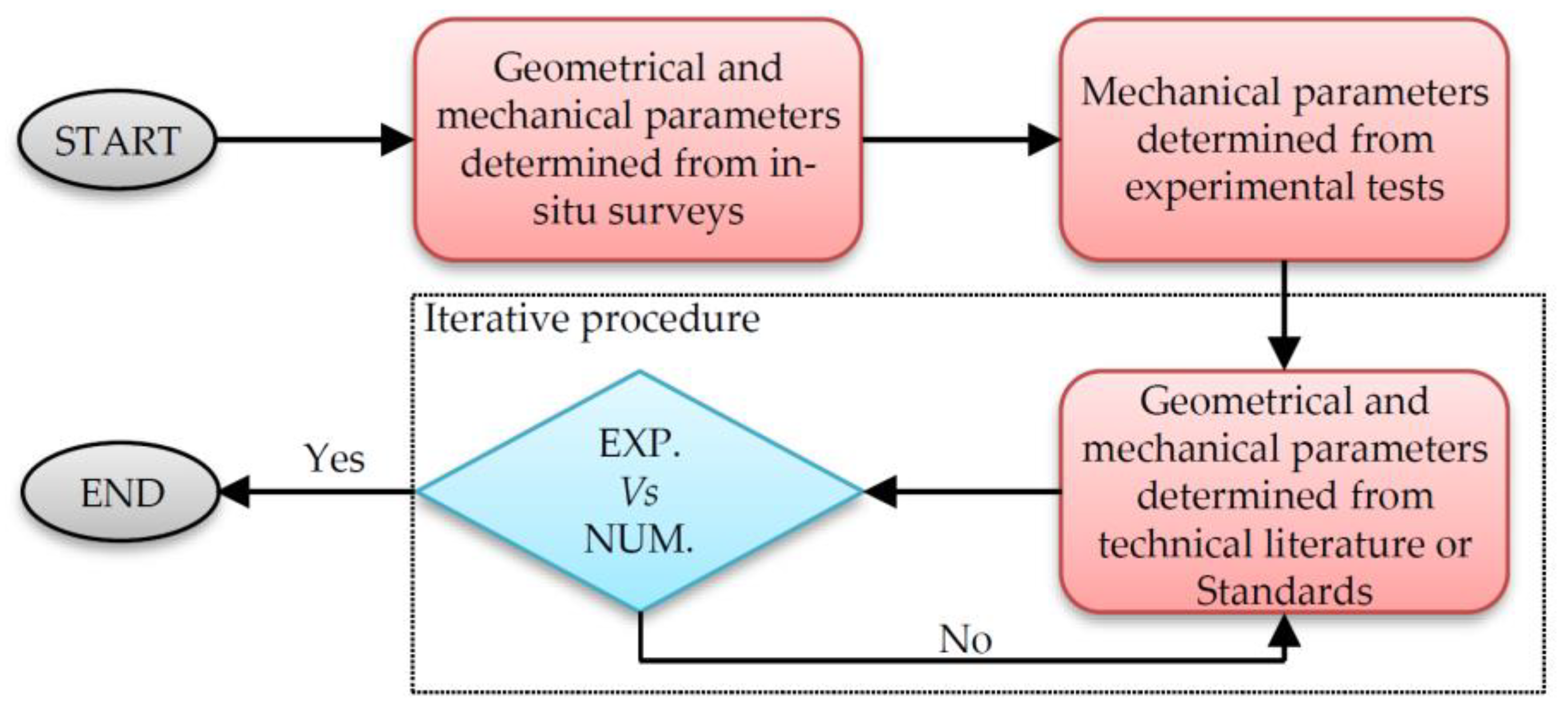
2. Modelling Strategies for the FEM Updating of Buildings

A calibrated FEM of a building permits us to obtain more realistic and trustworthy outcomes from the different numerical analyses that could be performed for various purposes [42,43]. The calibration is mostly performed based on the comparison between experimental and numerical responses. Nowadays, the main features compared in the model updating procedure are the modal parameters of the structure, namely frequencies, damping ratios, and mode shapes relevant to the vibration modes of the structure. Experimentally, these parameters are obtained through dynamic in-situ tests, along with the Ambient Vibration Tests (AVTs), are the most adopted [44]. These tests consist in measuring the vibrations (accelerations and/or velocities) on the structure produced by the so-called ambient noise (i.e., microtremors due to wind, waves, anthropic activities, such as traffic, works, etc.), and obtaining the real dynamic behaviour of the structure (i.e., modal parameters) thanks to suitable dynamic identification techniques [45]. Numerically, modal parameters can be obtained simply by performing linear modal analyses on the FEM. The comparison between experimental and numerical modes must be consistent; that is, differences in frequencies and mode shapes need to be reduced as much as possible. To assess the likeliness between mode shapes, the Modal Assurance Criterion (MAC) index [46] may be used; this index objectively shows the degree of similarity between two mode shapes through a numerical value ranging from 0 to 1: if 0, the mode shapes are completely different (orthogonal mode shapes), if equal to 1, the mode shapes are the same. Intermediate values indicate more or less accurate likeness.

The model updating is performed on varying geometrical and mechanical (mass and stiffnesses) parameters of the numerical model, sometimes adopting iterative procedures, and it can be considered concluded when the numerical modal parameters match the experimental ones. The model updating can be divided into direct and indirect methods [47,48]. The former involves reproducing data from the real structure by making minor adjustments to the stiffness and mass matrices without taking into account the change of physical parameters; the latter implies changing the model’s physical parameters until it accurately reproduces the data experimentally collected, and differences between experimental and numerical results are reduced to an allowable level. In this work, the second updating methodology is considered, even if iterative procedures are not adopted, since the proposed strategies generally avoid the need for such time consuming procedures. Indeed, the different parameters accounted for in the updating procedure, as well as the geometry of the models, are accurately estimated based on the outcomes of in-situ surveys and experimental tests and adopting suitable strategies, as better explained in the sequel. The proposed strategies can also be adopted to obtain reference values of modelling parameters and, consequently, to establish reliable and confident ranges to be assigned to these parameters during iterative updating procedures. In this sense, they permit reducing the possibility of finding false solutions, i.e., values of some parameters that provide a good numerical solution (making the numerical results match the experimental ones) but are far from their actual physical value.

During the indirect updating procedures, modifications are commonly made to the material mechanical properties (especially the elastic modulus and the mass density of the concrete [49]), to the load and mass applied to the structure, and to the restraint conditions. Moreover, modifications to the modelling strategies of some structural members can be made as well, also adding or deleting some structural components. Sometimes, it is also necessary to modify the geometry of the numerical model, adding some elements that were initially neglected, for example, some secondary structural components, nonstructural elements, and even surrounding structures that provide a sort of restraint to the considered one. In the sequel, the most relevant modelling strategies that can be adopted to calibrate FEMs of buildings are discussed in a general manner, starting from the common and simple FEM developed for design purposes. The parameters considered for the model updating are the following:

• geometry of the model and modelled elements;
• soil-structure interaction;
• concrete elastic modulus;
• modelling strategies for floor slabs;
• mechanical properties of infill masonry walls;
• load and mass.

Some of the above parameters can be varied based on experimental nondestructive test outcomes (i.e., concrete elastic modulus and mechanical properties of infills) or in-situ survey evidence (i.e., geometry, load, and mass). For other parameters, geometrical considerations can be made (i.e., floor slabs), and suggested values from technical literature or standards can be adopted (i.e., soil−structure interaction and concrete elastic modulus). Obviously, the precision of the estimated parameters depends on how they are obtained. If they are estimated based on experimental test results, the accuracy depends on the number and position of tests that should interest, as much as possible, the whole structure. If they are derived from the literature review, their accuracy may be verified only by comparing the global numerical model outcomes with the results of relevant experimental tests. In the latter case, plausible intervals can be defined and iterative procedures can be developed to find the best values for the structure at hand. A flowchart that summarizes the above considerations is reported in Figure 1.

2.1. The Common Design FEM

During the design phase of an edifice, a 3D FEM of the structure is always built based on architectural and structural drawings to support the structural calculation. Commonly, this model is rather simple, and very often, only the superstructure is modelled while the foundations are designed separately. In this case, the columns of the first elevation are fixed at the base. The structural elements of the RC frame (beams and columns) are modelled as beam elements, while RC slabs (e.g., stairs, ramps, walls, etc.) with shell or beam elements. The rigidity of the joints between beams and columns is considered, assigning rigid-end offsets determined according to the joint geometry and considering appropriate rigidity factors (a suggested value may be 0.5 [50]). The material properties for the concrete (modulus of elasticity, mass density, and compressive strength) are assumed to be the same for all the structural members; in particular, the elastic modulus is generally calculated starting from the design compressive strength and then reduced by 50% to account for the member cracking, as proposed in several codes [51,52]. Floor slabs are not modelled, but they are considered both in terms of load (usually assigned to the beams) and in terms of stiffness through floor constraints that simulate the in-plane rigidity of the slabs. Nonstructural elements (external and internal infills, screeds, floorings, ceilings, etc.) are generally considered only in terms of added load and mass. The load (and mass) applied to the model are those relevant to the design phase, namely the structural, nonstructural, live, and environmental load, properly combined according to the different code provisions.

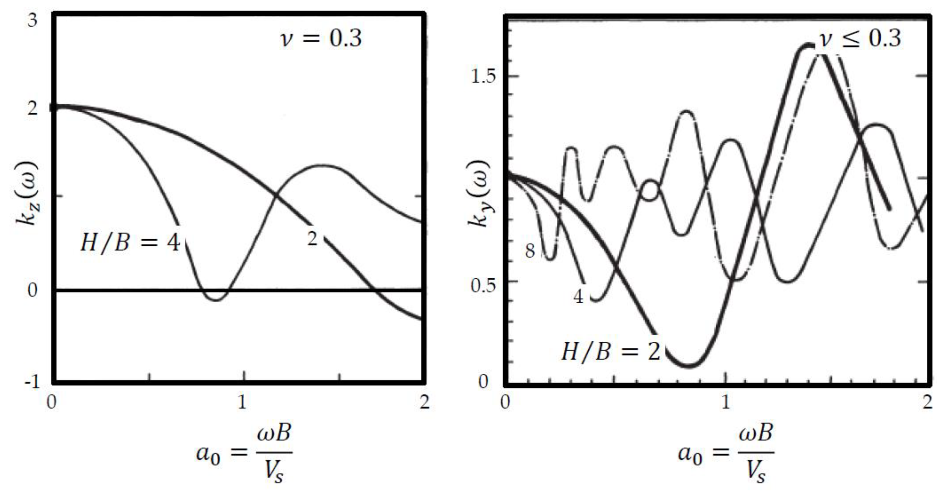
2.2. Modelling of the Soil-Structure Interaction

The hypothesis of the fixed base model often does not reflect the real condition of the structure. Indeed, even if it allows the highest actions on the superstructure to be obtained, it could lead to different dynamic properties of the structure than the real ones. Hence, for obtaining a calibrated FEM, modelling the structural foundation system becomes crucial, as well as the link with the surrounding ground (the so-called soil−structure interaction [53]). The structural foundation system can be modelled by adopting the beam element for both shallow and deep foundations (tie beams and piles), as well as shell elements for retaining walls that are connected to the structure, which sometimes form the basement floor. The soil−structure interaction can be accounted for by adopting, in the simplest approach, the Winkler model that consists of simulating the soil as distributed independent springs and assuming the pertinent soil dynamic parameters. The dynamic stiffness of springs can be calculated according to the structural element typology and using formulae available in the literature.

As concerns the foundation piles, the dynamic stiffness of vertical springs around the pile shaft (${\overline{K}}_{z,p}$ per unit length of pile) is calculated using the Gazetas and Makris [54] Equation (1):

$${\overline{K}}_{z,p}=0.6E_s$$

(1)

where $E_s$ is the soil elastic modulus. The pile base is pinned, being the soil under the pile comparable to a rigid bedrock. A simplified methodology to calculate the lateral dynamic response of piles is that proposed by Makris and Gazetas [55], which permits us to estimate the horizontal spring dynamic stiffness around the pile shaft (${\overline{K}}_{x,y,p}$ per unit length of pile) using Equation (2):

$${\overline{K}}_{x,y,p}=1.2E_s$$

(2)

The tie beams are considered as shallow foundations; hence the closed-form expressions and graphs reported in [56] are adopted to estimate the spring dynamic stiffnesses. In detail, the dynamic stiffness $\overline{K}\left(\omega \right)$ can be calculated as:

$$\overline{K}\left(\omega \right)=K·k\left(\omega \right)$$

(3)

with $K$ the static stiffness and $k\left(\omega \right)$ the dynamic stiffness coefficient. The former can be divided into two components: $K_{z,tb}$ and $K_{y,tb}$ (expressed per unit length of the element), which represent the vertical and lateral static stiffnesses, respectively; both of them are calculated supposing the element as a strip foundation placed on a homogeneous soil stratum, and using Equations (4a) and (4b):

$$K_{z,tb}=\frac{0.73G}{1-\nu }\left(1+3.5\frac{B}{H}\right)$$

(4a)

$$K_{y,tb}=\frac{2G}{2-\nu }\left(1+2\frac{B}{H}\right)$$

(4b)

where $G$ and $\nu$ are the soil shear modulus and Poisson’s coefficient, $B$ is the element half-width, $H$ is the soil stratum depth, and the ratio $H/B$ defines the relative depth to bedrock. The dynamic stiffness coefficients for the vertical ($k_z\left(\omega \right)$) and lateral ($k_y\left(\omega \right)$) stiffnesses are obtained through the graphs reported in Figure 2 as a function of the relative depth to bedrock $H/B$ and of a coefficient $a_0$, the latter calculated as a function of the circular frequency $\omega$, the shear-wave velocity $V_s$, and the element semi-width $B$. Hence, once known $\omega$, the dynamic stiffness coefficient can be rapidly determined since the other parameters refer to the foundation geometry and to the soil properties, the latter usually known from geotechnical surveys and in-situ tests. As the circular frequency $\omega$, for the sake of simplicity, it can be assumed the fundamental vibration frequency of the whole building, obtained experimentally from AVT results, since it is expected to be the one that mostly affects the dynamic behaviour of the building (mobilizing the majority of the participating mass).

The dynamic stiffness of springs related to the retaining walls is calculated, still using Equation (3), as reported in [56]. In this case, the static stiffness $K$ (per unit length of the element and still separated into the two components $K_{z,wall}$ and $K_{y,wall}$) is calculated starting from those for tie beams and considering the element fully embedded with a sidewall height $D$, adopting Equations (5a) and (5b):

$$K_{z,wall}=K_{z,tb}\left[1+0.2{\left(\frac{D}{B}\right)}^{\raisebox{1ex}{$2$}\!\left/ \!\raisebox{-1ex}{$3$}\right.}\right]\left(1+3.5\frac{D}{H-D}\right)$$

(5a)

$$K_{y,wall}=K_{y,tb}\left(1+0.5\frac{D}{B}\right)\left(1+1.5\frac{D}{H}\right)$$

(5b)

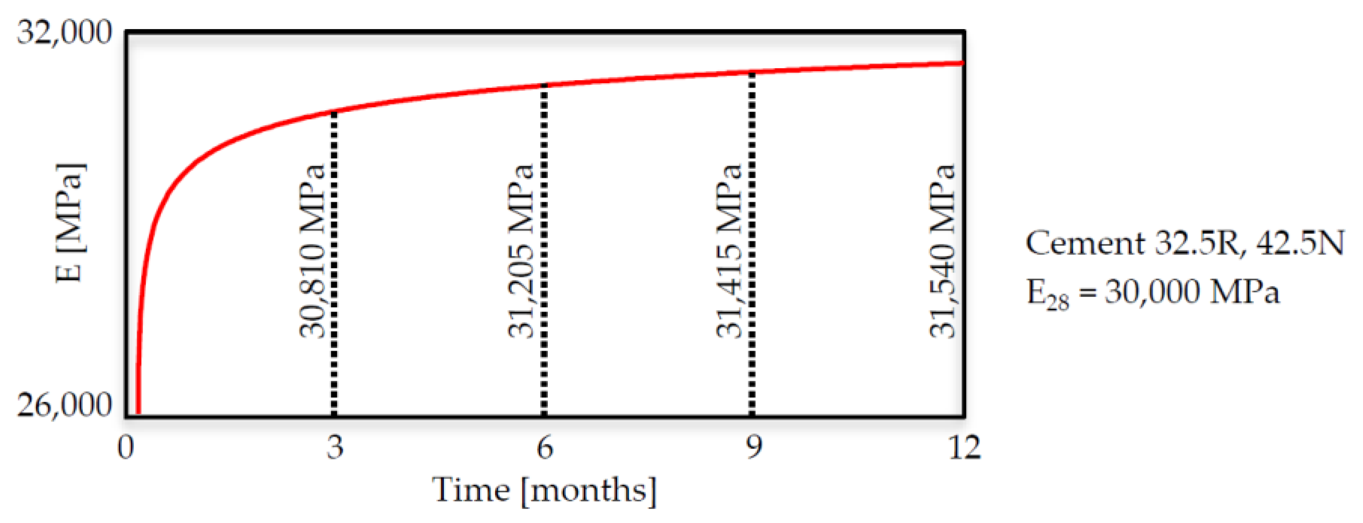
2.3. Modelling of the Experimental Value and the Time Evolution of Concrete Elastic Modulus

In cases in which the calibration procedure is based on AVT results, the concrete stiffness should be appropriately modified because the real building is energized by a very low input excitation (the ambient noise), which is not able to activate dissipative mechanisms within the building, such as the opening of concrete cracks. In these cases, the dynamic tangent elastic modulus ($E_d$) is considered instead of the common static secant one ($E_s$).

The dynamic elastic modulus can be calculated starting from the static one, as well as from experimental nondestructive tests on in-situ members, such as ultrasonic pulse tests. For the former case, literature relationships that correlate the dynamic elastic modulus with the static one can be adopted; indeed, $E_s$ can be easily calculated by adopting code formulae based on the concrete grade. Hence, once known the concrete design characteristics, $E_d$ can be simply determined based on literature correlations, as those reported in

Table 1. Relationships between $E_d$ and $E_s$ available in the literature.

Equations	Authors
$E_s=0.83E_d$	Lydon and Balendran [57]
$E_s=1.04E_d-4.1$ [GPa]	Swamy and Bandyopadhyay [58]
$E_s=k{E}_d^{1.4}{\rho }^{-1}$ [psi] $\rho$ concrete mass density [lbs/ft3] $k=0.23$	Popovics [59]
$E_d=1.5E_s-5.9$ [GPa]	Choudhauri et al. [60]

.

Considering experimental tests, the concrete is excited by means of ultrasonic waves or pulse-type loadings with a very high frequency, so the induced strain is smaller than the one developed during quasi-static compressive tests on specimens, and the elastic modulus appears larger than it actually is. It follows that the dynamic elastic modulus is representative almost exclusively of purely elastic effects since no microcracking or viscous effects occur during its measurement. The dynamic elastic modulus may be computed based on the pulse velocity ($V$) measured during ultrasonic pulse tests, and considering the wave propagation theory in homogeneous, isotropic, and elastic materials, which provides Equation (6):

$$E_d=\rho V^2\frac{\left(1+{\nu }_d\right)\left(1-2{\nu }_d\right)}{1-{\nu }_d}$$

(6)

where $\rho$ is the concrete mass density and ${\nu }_d$ is the dynamic Poisson coefficient (${\nu }_d$ = 0.28 is suggested in [59]).

The concrete elastic modulus can also be modified by taking into account the different aging periods of the many structural members that compose the whole building. Indeed, as is well known, the hardening of concrete over time (during the curing process) corresponds to an increase in stiffness. The concrete elastic modulus (both static and dynamic) at any time ($E\left(t\right)$) can be calculated based on Equation (7) [60], knowing the elastic modulus measured at day 28 from the casting ($E_{28}$):

$$E\left(t\right)={\left[{\beta }_{cc}\left(t\right)\right]}^{0.5}·E_{28}$$

(7)

where $t$ is expressed in days and ${\beta }_{cc}\left(t\right)$ is a coefficient that depends on the concrete aging, which can be calculated as follows:

$${\beta }_{cc}\left(t\right)=exp\left\{s·\left[1-{\left(\frac{28}{t}\right)}^{0.5}\right]\right\}$$

(8)

The coefficient $s$ is calculated considering the cement typology (strength class) and the concrete compressive strength, and may be taken according to Table 5.1-9 reported on page 86 of [61]. Considering the dynamic elastic modulus determined from ultrasonic pulse tests, if the latter is executed on in-situ members and at a different time from day 28 from casting, Equation (7) can be reversed, and $E_{28}$ is calculated being measured $E\left(t\right)$. Therefore, it is necessary to take at least one in-situ measurement for each casting phase and at any time to gain the elastic modulus variation over time, even if it is advisable to perform more measurements to obtain a more reliable experimental data set.

For the sake of completeness, a typical curve describing the elastic modulus evolution over time is reported in Figure 3. This is drawn considering 32.5R or 42.5N cement classes and assuming $E_{28}$ = 30,000 MPa. As can be observed, the elastic modulus markedly increases up to day 28, and then presents an asymptotic near-horizontal trend, denoting a very slow growth in stiffness. Hence, it is evident that differences in elastic modulus values must be considered when the updating procedure is performed on building FEMs that simulate the construction process while becoming almost negligible in the case of existing buildings.

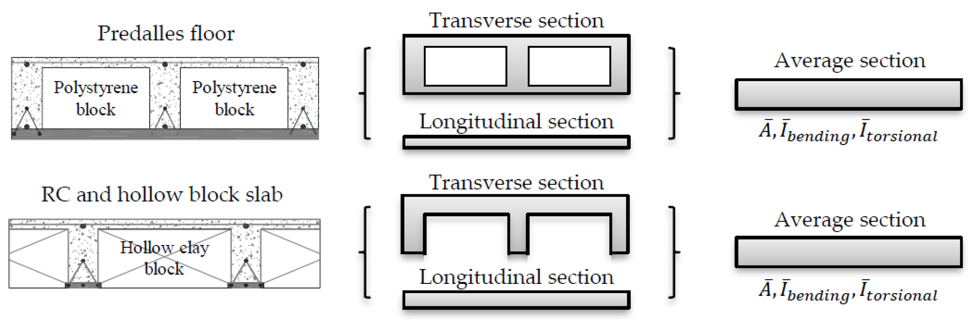
2.4. Modelling of the Floor Slabs

The floor slabs can be modelled within the FEM, adopting isotropic homogeneous shell elements that fill the planar space between the beams belonging to the same floor. Obviously, areas used for vertical connections (stairs, elevators, plant cavities, etc.) must be left empty. Floor modelling with shell elements becomes crucial where the plan shape of the building is not compact, but rather long; in this case, the in-plane deformation of the floor becomes significant and the in-plane rigid assumption is no longer valid. The thickness of the shell elements can be calculated in many ways; a common practice is adopting a mean thickness determined based on the construction typology of the floor slab. In fact, for RC floors, it is reasonable to assume for thickness the entire depth of the slab, whereas, in the case of floors constructed with RC and lightening components (e.g., hollow blocks), an equivalent mean thickness should be assumed, calculated considering only the contribution of the RC elements (RC slabs and ribs). In the latter case, the orthotropy of the plate should also be taken into account, especially in cases where the RC ribs are high with respect to the slab thickness. To do so, the geometrical property of the modelled shell elements (area and moments of inertia) can be suitably modified along the two main orthogonal directions. In cases where the mean thickness of the floor slab is considered, the floor mass must be separately calculated and then assigned to the modelled elements since the calculation performed by the software, also considering the element self-mass, leads to an erroneous mass estimation.

2.5. Modelling of the Nonstructural Elements

Nonstructural elements are commonly modelled within design FEMs as mass added to the structure. This assumption is rather appropriate when numerical analyses are performed considering extreme load conditions, so when only the structural components are supposed to provide resistance. However, the aforementioned hypothesis is no longer valid in buildings with infill walls since the latter provide a significant contribution also in terms of lateral stiffness to the structure. Therefore, it is crucial to consider the contributions of the walls both in terms of mass and stiffness when model updating of infilled RC buildings is faced. To do so, the infills must be modelled within the FEM; many modelling strategies can be found in the literature, along with the use of one or more equivalent diagonal struts, as well as the adoption of bidimensional shell elements. The first methodology has the great benefit of being quick and very simple to execute, while the second one allows for a more realistic modelling of the actual behaviour of the infills, even if it needs more care in the modelling and higher computational efforts in the analyses. A comprehensive review of these modelling strategies can be found in [44].

A possible strategy to consider the infill walls in the modelling of RC frame buildings is that proposed by Nicoletti et al. [62]. The external and internal infill walls are modelled within the numerical model as homogeneous isotropic shell elements, considering their location, dimension, and thickness and modelling the openings for windows and doors. The infill mass is estimated with good accuracy, especially for new buildings, being known as the adopted construction materials and thicknesses. On the contrary, the stiffness is more difficult to estimate. In their paper [62], the authors proposed a procedure for obtaining the elastic modulus of the infills to be used in the FEM and based on the comparison between the infill numerical out-of-plane modal parameters with the relevant experimental ones, the latter achieved by nondestructive dynamic impact tests on infills. These dynamic tests are nondestructive, i.e., they do not produce any kind of damage to the infills, and they are also rapid and easy to perform, becoming a convenient solution for both new and existing buildings. Furthermore, to apply this methodology, it is not necessary to test all the infills because it is a common practice to adopt similar infill typologies (in terms of construction material and thicknesses [63]) within a building. Therefore, the infill walls can be divided into homogeneous families, and only the most representative for each of them should be tested. The estimated parameters of the representative walls are then considered for all the walls belonging to the same category.

When the structural members are modelled with frame elements (beams and columns), it is important to consider that the modelled infills have greater dimensions (height and length) with respect to the real ones. For this reason, the infill mass (in terms of mass density $\rho$) and stiffness (in terms of elastic modulus $E$ obtained through the proposed procedure [62]) are suitably modified using Equations (9a) and (9b):

$${\rho }_m=\rho /{\lambda }^2$$

(9a)

$$E_m=E/{\lambda }^2$$

(9b)

where $\lambda$ is the panel dimension percentage increment from the real to the modelled one (Figure 4). For the sake of simplicity and for infills with similar length and height, the latter coefficient can be assumed to be the same for both the panel sides (${\lambda }_{mean}$).

2.6. Modelling of Load and Mass

As previously stated, the common FEM adopted for design purposes contains all the load that can be applied to the structure over its life (structural, nonstructural, live, and environmental load), and they are combined with amplifying (and sometimes reducing) coefficients. Conversely, during the calibration procedure, only the load and mass actually present on the building must be considered since the modal parameters sensibly vary as a function of the mass of the structure. Generally, live loads are deleted, or at least reduced with respect to values proposed by codes, which are upper bounds seldom present on the building. Also, environmental load (snow, wind, and temperature) has to be considered only if present and the same occurs for the seismic load. Moreover, if the model updating is performed to calibrate building FEMs during construction, the nonstructural load and components should be neglected or partially considered in accordance with the construction stage, as well as the structural components that have not been built yet. For instance, plants and equipment are the last elements generally placed on the structure, and consequently, their mass should be neglected during the construction process; the same applies to ceilings and infills. The mass relevant to these nonstructural components could be negligible or not, depending on the structural typology and the building use; so, considering or not this mass may sometimes lead to important errors in the updating procedures. Still considering the FEM updating during the construction of a building, the mass relevant to elements temporarily placed on the building should be considered as well, in particular, if their contribution is not marginal in comparison to the total mass of the floor on which they are located. This is the case of construction materials piled in areas on the floors, or even construction equipment, e.g., cranes, massive cement mixers, scaffolds, formworks, vehicles, etc.

3. FEM Updating of a Building Case Study during Construction Phases

The model updating strategies proposed in the previous section are herein applied with reference to a real building case study, with the target to obtain calibrated FEMs able to faithfully represent the real behaviour of the building, that is, a strategic construction, i.e., a fire station. Moreover, the building case study was controlled during its construction both numerically and experimentally [64], so a stepwise model updating is performed considering the different construction phases deemed as milestones for the whole construction process. More specifically, these phases can be divided into two groups representing (i) the bare RC frame construction (four construction stages), and (ii) the infill wall construction (four construction stages), the latter constituting the most important nonstructural elements for the building case study. A summary of the controlled construction phases with the relevant description is reported in

Table 2. Description of the construction phases of the building case study.

Construction of the Bare Frame		Construction of the Infill Walls
Date	Description	Date	Description
11 July 2016	Foundation system 1st and 2nd elevation columns/stairs 1st floor slab	12 September 2016	1st and 2nd elevations
29 July 2016	2nd floor slab 3rd elevation columns/stairs	26 September 2016	3rd elevation
22 August 2016	3rd floor slab 4th elevation columns/stairs	7 November 2016	4th elevation
25 August 2016	4th floor slab (roof)	6 April 2017	Building completed (all nonstructural elements and devices)

.

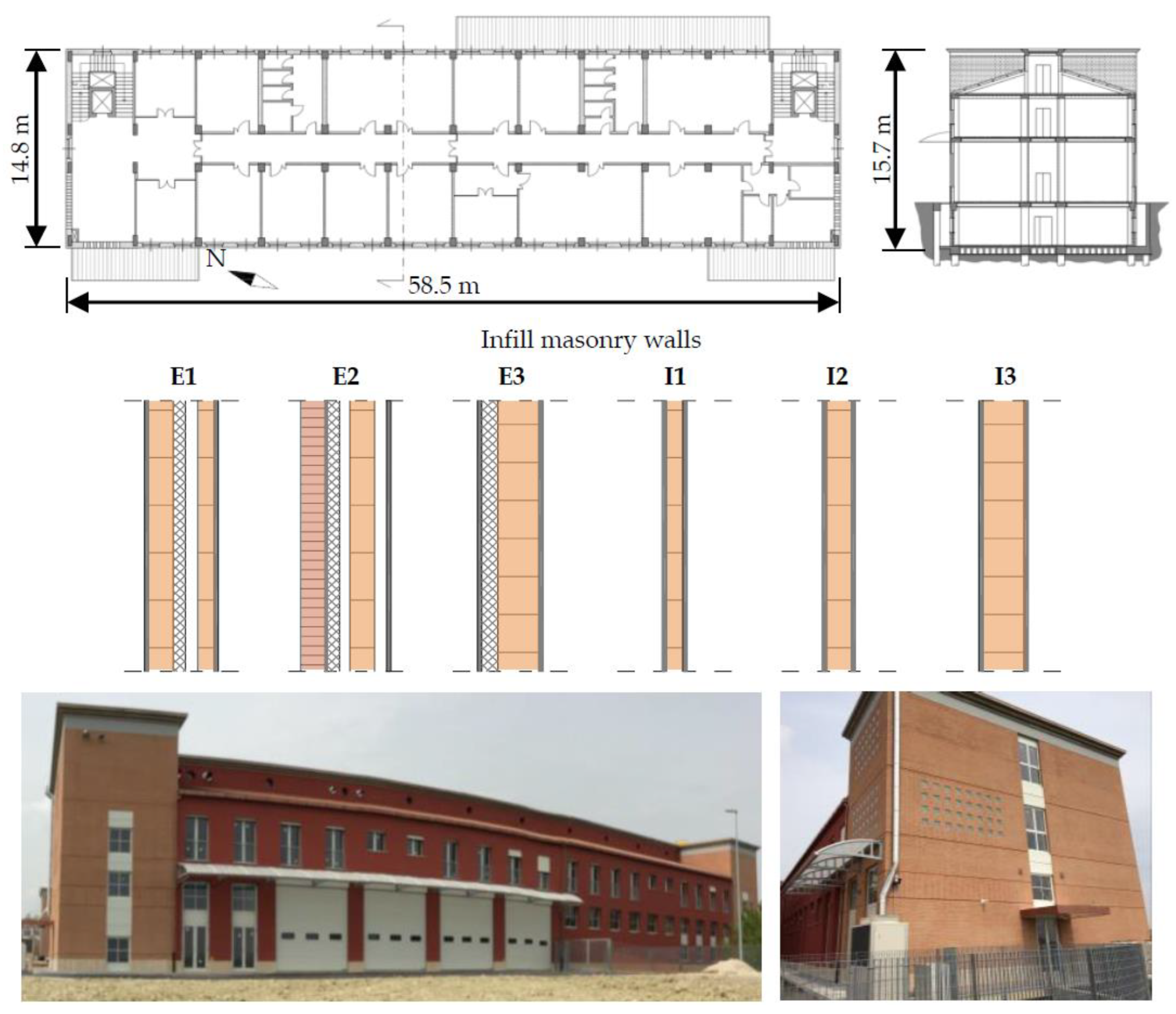
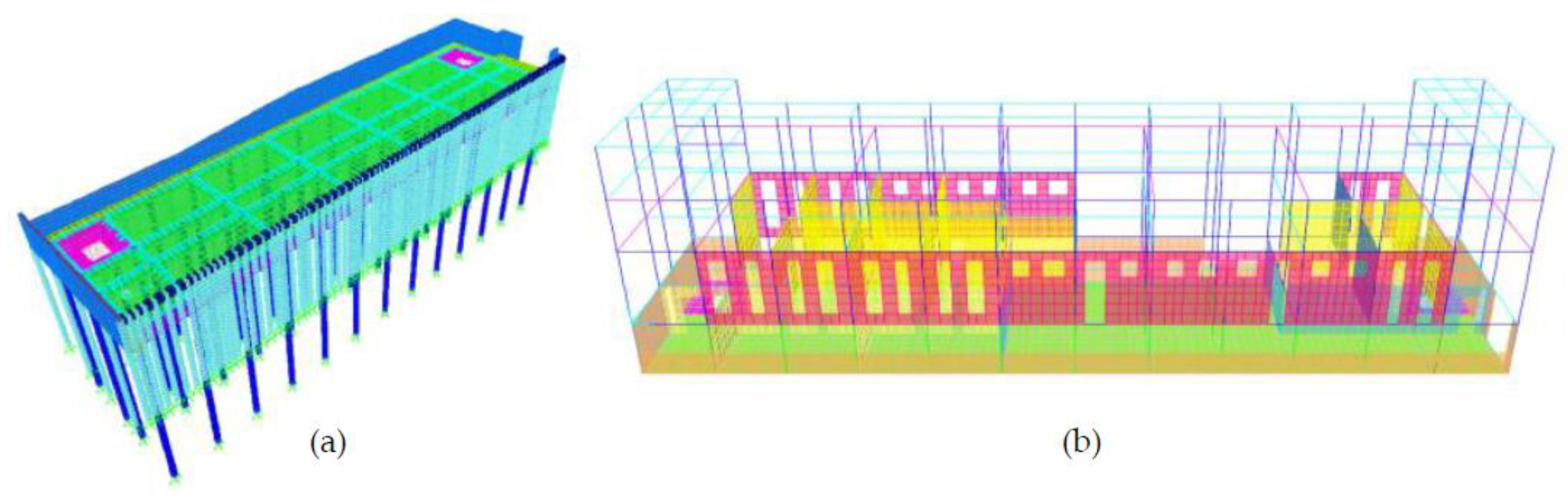
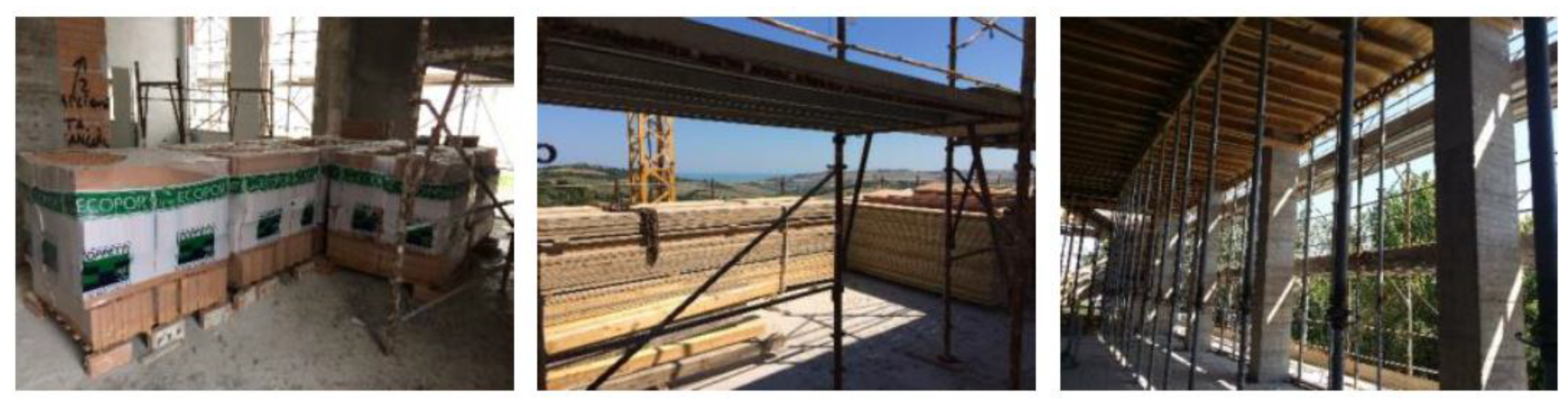
3.1. Building Description

The case study is a newly built infilled RC building located in Central Italy, with plan dimensions of about 59 × 15 m and a total height of about 16 m (3 storeys above the ground level and a basement) (Figure 5). The structural system constitutes RC beams and columns forming a spatial moment resisting frame and floor slabs that are realized with predalles element for the first two storeys, while there are hollow mixed floors for the last two. The structure has two RC staircases that rise around an elevator supported by a steel structure; the latter is separated from the RC frame. The building is founded on piles with a diameter of 0.60 m and a depth of 20 m. Tie beams (0.70 × 0.60 m cross-section) link the pile caps along the longitudinal and the transverse alignments. The contiguous pile wall on the west side of the building is made of drilled piles 0.50 m in diameter and 13 m long, with a head curb of 0.60 × 0.60 m cross-section dimensions. The pile wall is connected to the building with a 0.20 m thick RC slab that serves as an outdoor sidewalk at the ground level. On the other 3 sides of the building, retaining RC walls 0.30 m thick and 3.5 m high are built to separate the basement floor from the ground.

The soil characteristics have been investigated through in-situ geotechnical tests (4 continuous core drillings), through which it has been found that it mainly consists of marly clay soil characterized by a $V_s$ ranging between 180 and 360 m/s and elastic modulus around 410 MPa. The internal and external infills are realized with masonry walls built with hollow clay bricks and mortar joints. All the infills can be classified into six masonry families as a function of the adopted hollow clay bricks and the relevant thicknesses, as reported in Figure 5. The masonry belonging to the E1–E3 families are utilized to build all the external infill walls, while masonry I1–I3 are used to build all the interior partitions and those that separate the stairwells from the interior spaces. The building construction started on May 2016 and ended in April 2017.

3.2. Building FEM Updating

3.2.1. Common Design FEM Updating Considering Construction Phases

The design FEM of the building was developed by adopting the SAP2000 commercial software [65]. The first model was created for design purposes; therefore, it was rather simple and built with the same characteristics discussed in Section 2.1. In this FEM, the elevators are not modelled, because their steel structure is separated and disconnected from the RC frame. Then, this model is stepwise adjourned with the target to describe the actual behaviour of the structure in the different construction phases that are assumed for the construction process control; hence, eight calibrated FEMs are achieved (FEM1-FEM8), as reported in Figure 6.

At first, the geometry of the models is modified, deleting those structural elements that have not been built yet, specifically in the first three models (FEM1-FEM3). Moreover, the foundation system is modelled (Figure 7a), using frame elements for piles, tie beams, and the contiguous pile walls, whilst shell elements are adopted for the perimetric RC retaining walls. For the construction phases pertinent to FEM4–FEM8, the infill walls are inserted with shell elements taking into account the presence or not of the plaster. As stated in Section 2.5, all infills are modelled in their real position, with their thickness, and considering their openings, as can be observed in the example displayed in Figure 7b.

The elevators are not modelled since they are not linked to the building RC frame. A summary of the modelled structural and nonstructural elements at different construction phases is reported in

Table 3. Modelled structural and nonstructural elements at different construction phases.

Elements	FEM1	FEM2	FEM3	FEM4	FEM5	FEM6	FEM7	FEM8
Foundations & walls
1st elev. columns
1st floor slab
2nd elev. columns
2nd floor slab
3rd elev. columns
3rd floor slab
4th elev. columns
4th floor slab (roof)
1st elev. infills					YP	YP	YP	YP
2nd elev. infills					NP	NP	YP	YP
3rd elev. infills						NP	NP	YP
4th elev. infills							NP	YP

Yes modelled, Not modelled, NP = no plaster, YP = yes plaster.

.

3.2.2. Model Updating Considering the Soil−Structure Interaction

The soil−structure interaction is considered adopting the Winkler model, i.e., simulating the soil as distributed independent springs. The dynamic stiffness of these springs is calculated following the prescriptions reported in Section 2.2. For springs around the pile shafts, a constant value of the stiffness is assumed, calculated following Equations (1) and (2). Contrarily, the stiffnesses relevant to springs in tie beams and retaining walls also depend on the circular frequency $\omega$ of the structure, as previously stated; for simplicity it can be considered only the fundamental circular frequency of the building. However, this frequency varies during the building construction, so also the spring stiffnesses should vary for each of the eight FEMs. For the case study at hand, the fundamental frequency of the building varies approximatively around 2.6 to 6 Hz, as will be shown in the following sections, so the calculated parameter $a_0$ is always almost close to 0 since $V_s$ has a very high value compared with the product $\omega ·B$. Consequently, the dynamic stiffness coefficients are assumed to be the same for all the eight FEMs and equal to 1, meaning that, in this case, the dynamic stiffness almost coincides with the static one. A summary of the calculated dynamic stiffnesses for all the foundation elements is reported in

Table 4. Dynamic stiffness in [kN/m] for springs adopted to simulate the soil−structure interaction.

${\overline{\mathit{K}}}_{\mathit{z},\mathit{p}}$	${\overline{\mathit{K}}}_{\mathit{x},\mathit{y},\mathit{p}}$	${\overline{\mathit{K}}}_{\mathit{z},\mathit{t}\mathit{b}}\left(\mathit{\omega }\right)$	${\overline{\mathit{K}}}_{\mathit{y},\mathit{t}\mathit{b}}\left(\mathit{\omega }\right)$	${\overline{\mathit{K}}}_{\mathit{z},\mathit{w}\mathit{a}\mathit{l}\mathit{l}}\left(\mathit{\omega }\right)$	${\overline{\mathit{K}}}_{\mathit{y},\mathit{w}\mathit{a}\mathit{l}\mathit{l}}\left(\mathit{\omega }\right)$
6.15 × 104	12.4 × 104	26.3 × 104	19.3 × 104	17.7 × 104	26.1 × 104

.

3.2.3. Model Updating Considering the Experimental Value and Time Evolution of Concrete Elastic Modulus

The dynamic elastic modulus of concrete is considered instead of the static one, together with its evolution over time. Indeed, as stated in Section 2.3, different ages of concrete (and hence different concrete maturations) reflect in different concrete elastic moduli. The whole construction process inherent to the structural members can be divided into nine main casting phases (I to IX), as reported in

Table 5. Dynamic elastic moduli of the concrete ($E_d$) in [GPa] assumed for each of the eight FEMs.

N.	Elements	${\mathit{E}}_{28}$	FEM1	FEM2	FEM3	FEM4	FEM5	FEM6	FEM7	FEM8
I	Foundations	30.6	31.7	32.1	32.4	32.5	32.7	32.8	33.0	33.5
II	1st elev. columns	31.2	32.5	33.2	33.9	33.9	34.2	34.4	34.9	35.6
III	1st floor slab	31.5	31.1	32.6	33.6	33.7	34.2	34.4	35.0	36.0
IV	2nd elev. columns	29.7	28.1	30.3	31.5	31.6	32.1	32.4	32.9	33.8
V	2nd floor slab	32.0	---	30.3	33.0	33.2	34.0	34.4	35.2	36.3
VI	3rd elev. columns	31.4	---	27.6	31.9	32.1	33.1	33.6	34.5	35.6
VII	3rd floor slab	32.3	---	---	31.2	31.7	33.4	34.1	35.3	36.6
VIII	4th elev. columns	32.0	---	---	29.6	30.3	32.7	33.5	34.8	36.3
IX	4th floor slab (roof)	31.7	---	---	---	18.8	30.6	32.3	34.2	35.9

. Consequently, the structural members of the FEMs are classified into nine groups, and a dynamic elastic modulus of the concrete is assigned to each of them. Moreover, considering a single casting phase, the dynamic elastic modulus varies over time, following the relationship suggested in Equation (7). So, in each of the eight FEMs, the concrete elastic moduli are varied, adopting Equation (7), and the relevant values are listed in Table 5. Some structural elements belonging to different casting phases have been in-situ tested during the building construction, performing ultrasonic pulse tests, whose results (in terms of pulse velocities $V$) are reported in the work of Nicoletti et al. [64]. All tests were performed in only one day (30 September 2016), so the $E_{28}$ relevant to each casting phase is calculated, reversing Equation (7), being known the pouring dates ($t$). For the foundation system, it was not possible to perform any tests, so the $E_{28}$ is estimated based on the literature formulae reported in Table 1, being known the concrete design characteristics.

3.2.4. Model Updating Considering the Floor Slabs

The floor slabs are modelled with homogeneous isotropic shell elements because the elongated plan shape of the building suggests that the in-plane deformability of the floors may not be negligible. Being the latter realized with RC and lightening elements, the thicknesses of the relevant shells are calculated considering only the geometry of the RC members, and calculating a mean value between the two main orthogonal directions. An example of the mean thickness calculation is reported in Figure 8. The elastic modulus assigned to each floor is the same estimated for the beams belonging to the same storey. The floor mass is separately calculated and then assigned to the shells as added mass. An alternative way could consist in calculating a mean value of the mass density between concrete and lightening elements to be assigned to the shell element properties, but in this second case, the mass of each modelled floor is less refined. The orthotropy of the floors is considered as well. In particular, only the stiffness contribution of the RC elements is taken into account, being negligible that relevant to the lightening components.

Consequently, the cross sectional area and moments of inertia of the real floors without lightening are calculated and then compared with those of the rectangular cross-section shells, which are modified to be in accordance with the former (acting on multipliers of the geometrical properties).

3.2.5. Model Updating Considering the Nonstructural Elements

The mechanical properties of infills are estimated based on the procedure proposed by Nicoletti et al. [62]. Indeed, in-situ experimental dynamic tests have been performed on selected infills during the building construction both before (NP) and after (YP) the plaster realization since also this element may influence the mass and, most of all, the stiffness of the nonstructural components (details and results about the experimental campaign on infills are available in [64]). In this way, a refined and detailed infill wall modelling is obtained, especially for the FEMs referring to the building construction. The mass of infills is easily estimated being the construction materials known, as well as the geometry. The infill mechanical parameters are estimated for all six classes of masonry, and they are listed in

Table 6. Mechanical properties of the infill walls adopted in the modelling (to be reduced by ${\lambda }^2$).

Name	Plaster	Mass Density $\mathit{\rho }$ [kN/m3]	Elastic Modulus $\mathit{E}$ [MPa]	Thickness [cm]
E1	NP	5.8	3800	20
	YP	7	5000	24
E2	NP	13	7100	12
	YP	12	10,000	24
E3	NP	6.5	2600	20
	YP	7	4800	24
I1	NP	3.5	2400	8
	YP	7.5	4400	12
I2	NP	6	5100	12
	YP	8	6100	16
I3	NP	6.5	2600	20
	YP	7	4800	24

. These values are suitably adopted in the eight FEMs, also considering the presence or not of the plaster. It is worth noting that the values of Table 6 must be reduced by the ${\lambda }^2$ factor once entered into the model, as discussed in Section 2.5.

3.2.6. Model Updating Considering Actual Load and Mass

Finally, also the mass of the eight FEMs is modified considering for each construction phase the load actually present on the building. Live and environmental loads are neglected, and those referring to structural and nonstructural elements are considered without adopting code combination factors (i.e., without reductions or amplifications). For the latter, in-situ surveys have been performed at each construction phase, and detailed notes have been collected.

During these surveys, also the presence of added mass has been registered together with their location on the floors; the main added mass refer to masonry packages located in several positions on floors, as well as scaffolds and stacked formworks, as shown in Figure 9.

4. Validation of the FEM Updating for the Building Case Study

The assessment of the eight FEM updates is performed comparing the numerical modal parameters with the relevant experimental ones. The latter are achieved by in-situ AVTs performed at each of the eight main construction phases. A full description of these experimental test campaigns and results can be found in [64].

For the model updating validation, only the first three vibration modes for each construction phase are taken into account in this work, which are representative of the first longitudinal, transverse, and rotational modes, respectively. The comparison is made both in terms of natural frequencies and mode shapes, the latter adopting the MAC index between numerical and experimental mode shapes. For the latter, the modal displacements of the monitored points on the structure (sensor locations) are considered. Figure 10 and Figure 11 summarize this comparison and highlight the model updating correctness. Indeed, as can be seen, the numerical predictions are in very good agreement with the experimental results, with MAC values almost always higher than 0.8 (except for 1 value) and higher than 0.9 in most cases; maximum differences in frequency are about 9%. Furthermore,

Table 7. Comparison between frequencies obtained numerically (design FEM) and experimentally.

Numerical f [Hz] Design FEM	Experimental f [Hz] Bare Frame	Experimental f [Hz] Complete Building
1.63	2.62	6.02
1.93	3.40	6.42
2.52	4.19	7.06

still proposes the comparisons in terms of frequencies, but in this case, considering the design numerical model. The outcomes of the numerical model are compared with the experimental values relevant to both the bare frame structure (i.e., the experimental counterpart of FEM4) and the complete building (i.e., the experimental counterpart of FEM8). As expected, this model does not fit the experimental outcomes in both cases because it is developed for the calculation of the structure at the ultimate limit states, adopting all the simplified assumptions that are reviewed in the proposed refining strategies.

Summarizing, accurate FEMs that faithfully represent the behaviour of the building during its construction process have been obtained starting from the common design FEM and using the suggested updating strategies. The latter do not require much effort in their application because they are based on known structural aspects. At the same time, they avoid the use of iterative processes with automatic calibration algorithms whose results (calibrated parameters) may sometimes be difficult to interpret from a structural and physical point of view.

5. Conclusions

The paper proposed modelling strategies to be applied for the updating of FEMs of infilled RC buildings. Moreover, methodologies to update models during the construction process of a building have been provided as well.

• At first, the modelling strategies to refine FEMs are treated, starting from the common design FEM, which is usually very simple and built considering manifold simplifying assumptions. Recommendations about how to accurately model the geometry of the buildings, the soil−structure interaction, the elastic modulus of concrete, the floor slabs, the infill walls, and the actual load and mass on the structure are reported.
• The evolution of the above parameters during the construction process of a building is addressed as well, proposing modelling strategies to be adopted for modelling a building during its construction.
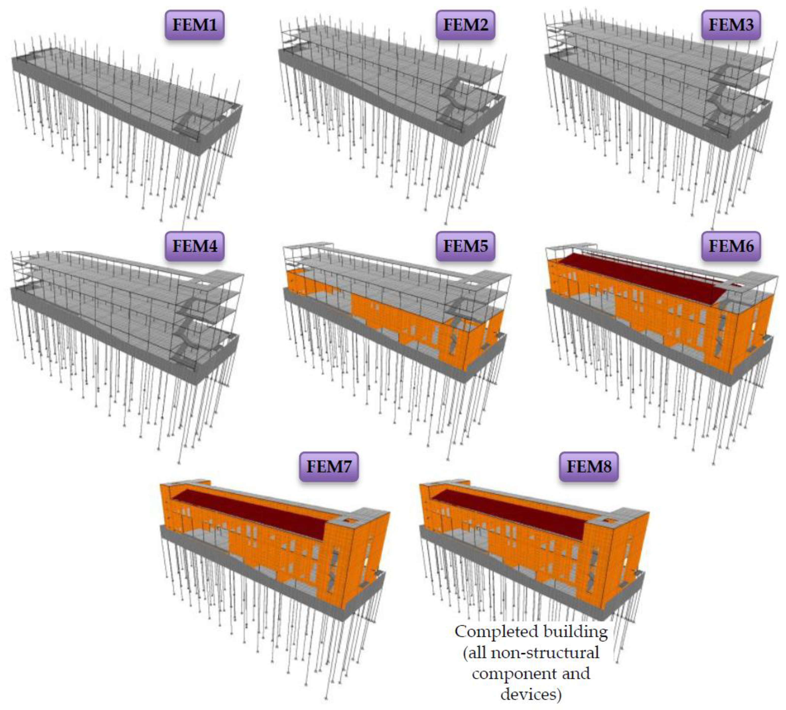
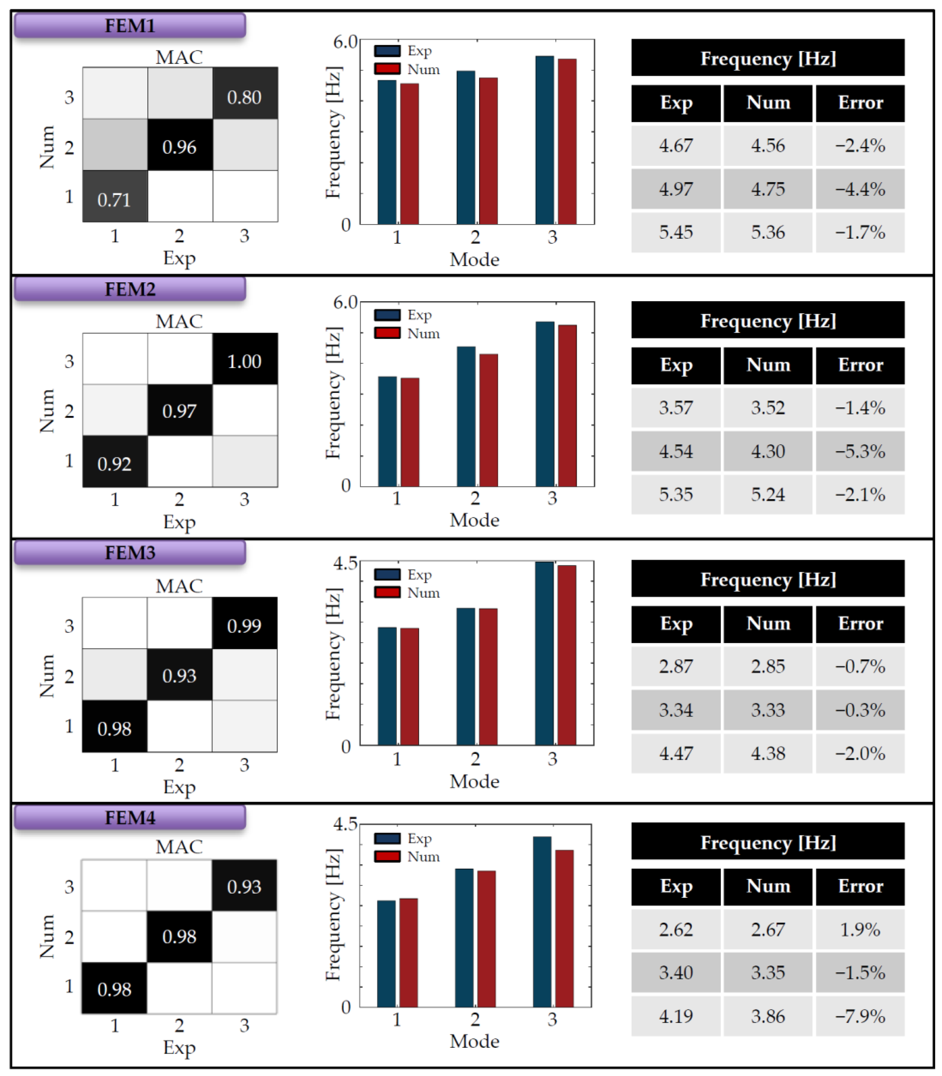
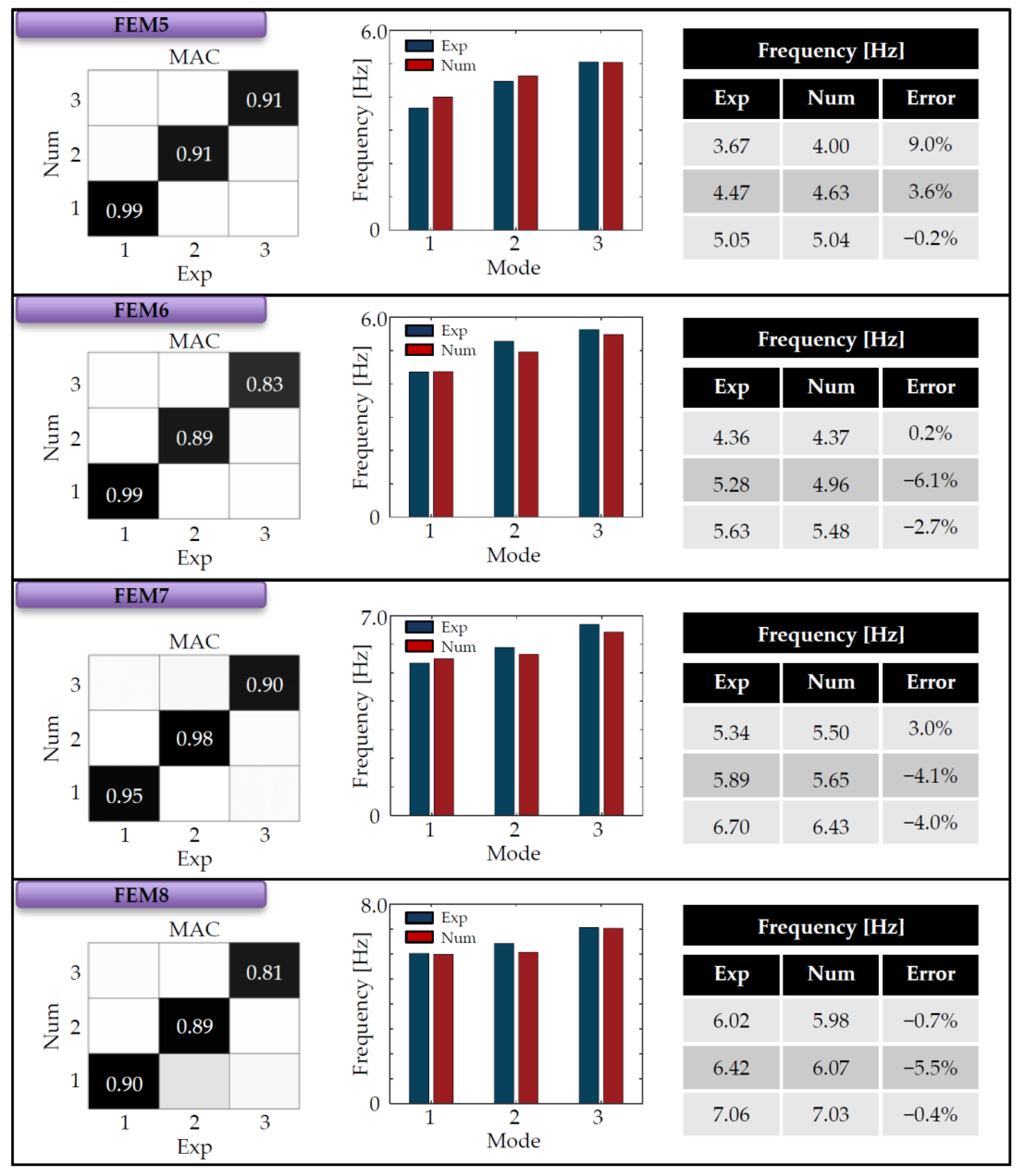
• An application to a real building case study is provided at the end. The considered building has been widely investigated during its construction, also performing static and dynamic in-situ tests that allowed the determination of the global dynamics, as well as the mechanical properties of the construction materials and components. A stepwise model updating adopting the proposed modelling strategies is then performed, realizing and updating eight FEMs that represent the eight main construction phases. The numerical outcomes reached from the eight models are compared with the relevant experimental ones, and the comparison shows a very good agreement, demonstrating the effectiveness of the proposed model updating strategies and the correctness of the construction procedure for the building at hand.

The model updating method adopted in this work is the so-called indirect method, i.e., the physical parameters of the models are adjusted until the convergence between numerical and experimental outcomes is reached. However, iterative procedures in the estimation of the physical parameter values are not performed since good results are achieved by adopting precise strategies supported by in-situ surveys and nondestructive test outcomes.

The proposed updating strategies are of great support when calibrated FEMs are necessary to perform particular analyses or investigations. For instance, a calibrated FEM can support the design of an SHM system, as well as the interpretation of its outcomes. Moreover, a model that faithfully represents the behaviour of the real structure can be used to investigate possible damage scenarios due to exceptional events and, consequently, to determine admissible thresholds on selected parameters that must be controlled during the building life. Also, a calibrated model is one of the main components required for the development of digital twins of buildings, supporting the management and maintenance of the structures. Finally, the model updating during the construction of a building may provide a crucial tool for controlling the construction correctness and performing intermediate numerical analyses to support the construction activities, especially for large and complex buildings. All the above considerations hold, for example, in the case of strategic constructions.

The modelling strategies proposed in this study can be applied in all buildings with the same construction typology (and similar ones), so they configure as a sort of guidance for the model updating procedure. Moreover, in the case of iterative updating, the proposed methods for estimating the material mechanical properties can be adopted to obtain reference values useful for establishing plausible ranges of variation of these parameters, hence leading to a more aware updating procedure and more reliable results.

References

1. Mottershead, J.E.; Link, M.; Friswell, M.I. The sensitivity method in finite element model updating: A tutorial. Mech. Sist. Signal Proc. 2011, 25, 2275–2296. [Google Scholar] [CrossRef]
2. Mottershead, J.E.; Friswell, M.I. Model updating in structural dynamics: A survey. J. Sound. Vib. 1993, 167, 347–375. [Google Scholar] [CrossRef]
3. Blaz, K.; Bostjan, B.; Wai Kei, A. Model updating of seven-storey cross-laminated timber building designed on frequency-response-functions-based modal testing. Struct. Infrastruct. Eng. 2023, 19, 178–196. [Google Scholar] [CrossRef]
4. Garcia-Marcias, E.; Ierimonti, L.; Venanzi, I.; Ubertini, F. An innovative methodology for online surrogate-based model updating of historic buildings using monitoring data. Int. J. Arch. Herit. 2021, 15, 92–112. [Google Scholar] [CrossRef]
5. Ceravolo, R.; De Lucia, G.; Miraglia, G.; Pecorelli, M.L. Thermoelastic finite element model updating with application to monumental buildings. Comput. Aided Civil Infr. Eng. 2020, 35, 628–642. [Google Scholar] [CrossRef]
6. Imregun, M.; Sanliturk, K.Y.; Ewins, D.J. Finite element model updating using frequency response function data–I, Theory and initial investigation. Mech. Syst. Sig. Process. 1995, 9, 187–202. [Google Scholar] [CrossRef]
7. Sivori, D.; Lepidi, M.; Cattari, S. Structural identification of the dynamic behaviour of floor diaphragms in existing buildings. Smart Struct. Syst. 2021, 27, 173–191. [Google Scholar] [CrossRef]
8. Falcone, R.; Lima, C.; Martinelli, E. Soft computing techniques in structural and earthquake engineering: A literature review. Eng. Struct. 2020, 207, 110269. [Google Scholar] [CrossRef]
9. Salehi, H.; Burgueno, R. Emerging artificial intelligence methods in structural engineering. Eng. Struct. 2018, 171, 170–189. [Google Scholar] [CrossRef]
10. Ierimonti, L.; Venanzi, I.; Cavalagli, N.; Comodini, F.; Ubertini, F. An innovative continuous Bayesian model updating method for base-isolated RC buildings using vibration monitoring data. Mech. Syst. Sig. Process. 2020, 139, 106600. [Google Scholar] [CrossRef]
11. Akhlaghi, M.M.; Bose, S.; Green, P.L.; Babak, M.; Stavridis, A. Bayesian model updating of a five-story building using Zero-Variance sampling method. In Proceedings of the Society for Experimental Mechanics Series–37th IMAC, A Conference and Exposition on Structural Dynamics, Orlando, FL, USA, 28–31 January 2019. Code 225789. [Google Scholar]
12. Lam, H.-F.; Hu, J.; Zhang, F.-L.; Ni, Y.-C. Markov chain Monte Carlo-based Bayesian model updating of a sailboat-shaped building using a parallel technique. Eng. Struct. 2019, 193, 12–27. [Google Scholar] [CrossRef]
13. Rosati, I.; Fabbrocino, G.; Rainieri, C. A discussion about the Douglas-Reid model updating method and its prospective application to continuous vibration-based SHM of a historical building. Eng. Struct. 2022, 273, 115058. [Google Scholar] [CrossRef]
14. Boscato, G.; Russo, S.; Ceravolo, R.; Fragonara, L.Z. Global sensitivity-based model updating for heritage structures. Comput. Aided Civ. Inf. 2015, 30, 620–635. [Google Scholar] [CrossRef]
15. Aloiso, A.; Pasca, D.; Tomasi, R.; Fragiacomo, M. Dynamic identification and model updating of an eight-storey CLT building. Eng. Struct. 2020, 213, 110593. [Google Scholar] [CrossRef]
16. Pan, Y.; Ventura, C.E.; Xiong, H.; Zhang, F.-L. Model updating and seismic response of a super tall building in Shanghai. Comput. Struct. 2020, 239, 106285. [Google Scholar] [CrossRef]
17. Gentile, C.; Saisi, A. FE modeling of a historic masonry tower and vibration-based systematic model tuning. Adv. Mat. Res. 2010, 133–134, 435–440. [Google Scholar] [CrossRef]
18. Foti, D.; Gattulli, V.; Potenza, F. Output-only identification and model updating by dynamic testing in unfavorable conditions of a seismically damaged building. Comput. Aided Civil Infr. Eng. 2014, 29, 659–675. [Google Scholar] [CrossRef]
19. Astroza, R.; Alessandri, A. Effects of model uncertainty in nonlinear structural finite element model updating by numerical simulation of building structures. Struct. Control Health Monit. 2019, 26, e2297. [Google Scholar] [CrossRef]
20. United States Geological Survey, USGS. Available online: https://www.usgs.gov/news/featured-story/magnitude-78-earthquake-nurdagi-turkey (accessed on 6 February 2022).
21. Bovo, M.; Tondi, M.; Savoia, M. Infill Modelling Influence on Dynamic Identification and Model Updating of Reinforced Concrete Framed Buildings. Adv. Civ. Eng. 2020, 2020, 9384080. [Google Scholar] [CrossRef]
22. Pepe, V.; De Angelis, A.; Pecce, M.R. Damage assessment of an existing RC infilled structure by numerical simulation of the dynamic response. J. Civ. Struct. Health Monit. 2019, 9, 385–395. [Google Scholar] [CrossRef]
23. Nicoletti, V.; Arezzo, D.; Carbonari, S.; Gara, F. Detection of infill wall damage due to earthquakes from vibration data. Earthq. Eng. Struct. Dyn. 2023, 52, 460–481. [Google Scholar] [CrossRef]
24. Kammer, D.C. Sensor placement for on-orbit modal identification and correlation of large space structures. J. Guid. Control. Dyn. 1991, 14, 251–259. [Google Scholar] [CrossRef]
25. Taher, S.A.; Li, J.; Fang, H. Simultaneous seismic input and state estimation with optimal sensor placement for building structures using incomplete acceleration measurements. Mech. Syst. Sig. Proc. 2023, 188, 110047. [Google Scholar] [CrossRef]
26. Zhou, Z.; Zhao, X.; Chong, P.H.J. Optimal relay node placement in wireless sensor network for smart buildings metering and control. In Proceedings of the 2013 15th IEEE International Conference on Communication Technology, Guilin, China, 17–19 November 2013; pp. 456–461. [Google Scholar] [CrossRef]
27. Kalakonas, P.; Silva, V. Earthquake scenarios for building portfolios using artificial neural networks: Part II—Damage and loss assessment. Bull. Earthq. Eng. 2022. [Google Scholar] [CrossRef]
28. Zeng, D.; Zhang, H.; Wang, C. Modelling correlated damage of spatially distributed building portfolios under scenario tropical cyclones. Struct. Saf. 2020, 87, 101978. [Google Scholar] [CrossRef]
29. Ventura, A.; De Biagi, V.; Chiaia, B. Structural robustness of RC frame buildings under threat-independent damage scenarios. Struct. Eng. Mech. 2018, 65, 689–698. [Google Scholar] [CrossRef]
30. Gara, F.; Arezzo, D.; Nicoletti, V.; Carbonari, S. Monitoring the Modal Properties of an RC School Building during the 2016 Central Italy Seismic Swarm. J. Struct. Eng. (ASCE) 2021, 147, 05021002. [Google Scholar] [CrossRef]
31. Bronkhorst, A.J.; Moretti, D.; Geurts, C.P.W. Vibration Threshold Exceedances in the Groningen Building Vibration Monitoring Network. Front. Built Environ. 2021, 7, 703247. [Google Scholar] [CrossRef]
32. Zong, Y.; Wan, F.; Hua, Y.; Liao, B.; Zhu, S.; Zhu, S. EEMD-Wavelet Adaptive Threshold Function Denoising and Its Application in Damage Monitoring of Aviation Connection Structure. In Proceedings of the 2021 Global Reliability and Prognostics and Health Management, PHM-Nanjing, Nanjing, China, 15–17 October 2021; p. 174772. [Google Scholar] [CrossRef]
33. Bado, M.F.; Tonelli, D.; Poli, F.; Zonta, D.; Casas, J.R. Digital Twin for Civil Engineering Systems: An Exploratory Review for Distributed Sensing Updating. Sensors 2022, 22, 3168. [Google Scholar] [CrossRef]
34. Nicoletti, V.; Martini, R.; Carbonari, S.; Gara, F. Operational Modal Analysis as a Support for the Development of Digital Twin Models of Bridges. Infrastructures 2023, 8, 24. [Google Scholar] [CrossRef]
35. Shim, C.-S.; Dang, N.-S.; Lon, S.; Jeon, C.-H. Development of a bridge maintenance system for prestressed concrete bridges using 3D digital twin model. Struct. Infrastruct. Eng. 2019, 15, 1319–1332. [Google Scholar] [CrossRef]
36. Tedjo, C.; Berawi, M.A.; Sari, M. Development of Blockchain and Machine Learning System in the Process of Construction Planning Method of the Smart Building to Save Cost and Time. In Proceedings of the 5th International Conference on Rehabilitation and Maintenance in Civil Engineering, ICRMCE, Surakarta, Indonesia, 8–9 July 2021; p. 282689. [Google Scholar] [CrossRef]
37. Andrich, W.; Daniotti, B.; Pavan, A.; Mirarchi, C. Check and Validation of Building Information Models in Detailed Design Phase: A Check Flow to Pave the Way for BIM Based Renovation and Construction Processes. Buildings 2022, 12, 154. [Google Scholar] [CrossRef]
38. Liu, Z.; Xing, Z.; Huang, C.; Du, X. Digital twin modeling method for construction process of assembled building. Jianzhu Jiegou Xuebao/J. Build. Struct. 2021, 42, 213–222. [Google Scholar] [CrossRef]
39. Wang, Z.; Huang, M.; Gu, J. Temperature effects on vibration-based damage detection of a reinforced concrete slab. Appl. Sci. 2020, 10, 2869. [Google Scholar] [CrossRef] [Green Version]
40. Zhou, Y.; Zhou, Y.; Yi, W.; Chen, T.; Tan, D.; Mi, S. Operational modal analysis and rational finite-element model selection for ten high-rise buildings based on on-site ambient vibration measurements. J. Perform. Constr. Facil. 2017, 31, 04017043. [Google Scholar] [CrossRef] [Green Version]
41. Astroza, R.; Ebrahimian, H.; Conte, J.P.; Restrepo, J.I.; Hutchinson, T.C. Influence of the construction process and nonstructural components on the modal properties of a five-story building. Earthq. Eng. Struct. Dyn. 2016, 45, 1063–1084. [Google Scholar] [CrossRef]
42. Kokalanov, V.; Trifunac, M.D.; Gicev, V.; Kocaleva, M.; Stojanova, A. High frequency calibration of a finite element model of an irregular building via ambient vibration measurements. Soil Dyn. Earthq. Eng. 2022, 153, 107005. [Google Scholar] [CrossRef]
43. Butt, F.; Omenzetter, P. Finite element model calibration of an instrumented RC building based on seismic excitation including non-structural components and soil-structure-interaction. In Proceedings of the 22nd Australasian Conference on the Mechanics of Structures and Materials, ACMSM 2012, Sydney, Australia, 11–14 December 2012; p. 98302, ISBN 978-041563318-5. [Google Scholar]
44. Nicoletti, V.; Arezzo, D.; Carbonari, S.; Gara, F. Vibration-Based Tests and Results for the Evaluation of Infill Masonry Walls Influence on the Dynamic Behaviour of Buildings: A Review. Arch. Comput. Methods Eng. 2022, 29, 3773–3787. [Google Scholar] [CrossRef]
45. Van Overschee, P.; De Moor, B. Subspace Identification for Linear Systems: Theory–Implementation–Applications; Kluwer Academic Publishers: Dordrecht, The Netherlands, 1996. [Google Scholar]
46. Allemang, R.J.; Brown, D.L. A correlation coefficient for modal vector analysis. In Proceedings of the 1st Int. Modal Analysis Conference, Bethel, CT, USA, 8–10 November 1982; pp. 110–115. [Google Scholar]
47. Friswell, M.I.; Inman, D.J.; Pilkey, D.F. Direct updating of damping and stiffness matrices. AIAA J. 1998, 36, 491–493. [Google Scholar] [CrossRef] [Green Version]
48. Carvalho, J.; Datta, B.N.; Gupta, A.; Lagadapati, M. A direct method for model updating with incomplete measured data and without spurious modes. Mech. Syst. Signal Process. 2007, 21, 2715–2731. [Google Scholar] [CrossRef]
49. Rezvan, S.; Moradi, M.J.; Dabiri, H.; Daneshvar, K.; Karakouzian, M.; Farhangi, V. Application of Machine Learning to Predict the Mechanical Characteristics of Concrete Containing Recycled Plastic-Based Materials. Appl. Sci. 2023, 13, 2033. [Google Scholar] [CrossRef]
50. Léger, P.; Paultre, P.; Nuggihalli, R. Elastic analysis of frames considering panel zones deformations. Comput. Struct. 1991, 39, 689–697. [Google Scholar] [CrossRef]
51. EN 1992-1-1; Design of Concrete Structures–Part 1-1: General Rules and Rules for Buildings. European Committee for Standardization (CEN): Brussels, Belgium, 2015.
52. D.M.17.01.2018; Aggiornamento delle «Norme Tecniche per le Costruzioni». Ministero Rome, Italy delle Infrastrutture e dei Trasporti: Rome, Italy, 2018. (In Italian)
53. Carbonari, S.; Dezi, F.; Gara, F.; Leoni, G. Seismic response of reinforced concrete frames on monopile foundations. Soil Dyn. Earthq. Eng. 2014, 67, 326–344. [Google Scholar] [CrossRef]
54. Gazetas, G.; Makris, N. Dynamic pile-soil-pile interaction. Part I: Analysis of axial vibration. Earthq. Eng. Struct. Dyn. 1991, 20, 115–132. [Google Scholar] [CrossRef]
55. Makris, N.; Gazetas, G. Dynamic pile-soil-pile interaction. Part II: Lateral and seismic response. Earthq. Eng. Struct. Dyn. 1992, 21, 145–162. [Google Scholar] [CrossRef]
56. Gazetas, G. Foundation vibrations. In Foundation Engineering Handbook; Fang, H.-Y., Ed.; Springer: Berlin/Heidelberg, Germany, 1991. [Google Scholar]
57. Lydon, F.D.; Balendran, R.V. Some observations on elastic properties of plain concrete. Cem. Concr. Res. 1986, 16, 314–324. [Google Scholar] [CrossRef]
58. Neville, A.M. Properties of Concrete, 5th ed.; The Royal Accademy of Engineering; Pearson: London, UK, 2011. [Google Scholar]
59. Popovics, J.S.; Zemajtis, J.; Shkolnik, I. ACI-CRC Final Report—“A Study of Static and Dynamic Modulus of Elasticity of Concrete”; ACI-American Concrete Institute: Urbana, IL, USA, 2008. [Google Scholar]
60. Choudhauri, N.K.; Kumar, A.; Kumar, Y.; Gupta, R. Evaluation of elastic moduli of concrete by ultrasonic velocity. In Proceedings of the National Seminar of ISNT, Chennai, India, 5–7 December 2002. [Google Scholar]
61. Fédération Internationale du Béton (fib). Fib Model Code for Concrete Structures 2010; Ernst & Sohn: Berlin, Germany, 2013. [Google Scholar]
62. Nicoletti, V.; Arezzo, D.; Carbonari, S.; Gara, F. Expeditious methodology for the estimation of infill masonry wall stiffness through in-situ dynamic tests. Constr. Build. Mater. 2020, 262, 120807. [Google Scholar] [CrossRef]
63. Li, H.; Li, J.; Farhangi, V. Determination of piers shear capacity using numerical analysis and machine learning for generalization to masonry large scale walls. Structures 2023, 49, 443–466. [Google Scholar] [CrossRef]
64. Nicoletti, V.; Arezzo, D.; Carbonari, S.; Gara, F. Dynamic monitoring of buildings as a diagnostic tool during construction phases. J. Build. Eng. 2022, 46, 103764. [Google Scholar] [CrossRef]
65. SAP2000 Advanced; Static and Dynamic Finite Element Analysis of Structures. CSI Computer & Structures, Inc.: Berkeley, NJ, USA, 2021.
Figure 1. Flowchart describing the modelling strategies to be adopted within a framework for the building model updating.
Buildings 13 00598 g001
Figure 2. Dynamic coefficients for the calculation of the vertical ( k z ( ω ) ) and lateral ( k y ( ω ) ) stiffness [56].
Buildings 13 00598 g002
Figure 3. Variation of elastic modulus over time (calculated following [61]).
Buildings 13 00598 g003
Figure 4. Geometrical assumption for the infill modelling within a frame structure.
Buildings 13 00598 g004
Figure 5. Construction details and pictures of the building case study.
Buildings 13 00598 g005
Figure 6. Eight FEMs representing the 8 controlled phases during the building construction.
Buildings 13 00598 g006
Figure 7. Modelling details: (a) foundation system, (b) infill walls of the first elevation.
Buildings 13 00598 g007
Figure 8. Modelling strategies for the floor slabs.
Buildings 13 00598 g008
Figure 9. Examples of added mass considered in the FEM updating.
Buildings 13 00598 g009
Figure 10. Comparison between experimental and numerical modal parameters after the updating—Part 1/2.
Buildings 13 00598 g010
Figure 11. Comparison between experimental and numerical modal parameters after the updating—Part 2/2.
Buildings 13 00598 g011