Feasibility of Automated Black Ice Segmentation in Various Climate Conditions Using Deep Learning

Abstract

Black ice has recently been identified as a major cause of transportation accidents due to detecting difficulties on the road surface. It is crucial to provide traffic users with black ice warnings beforehand to sustain commuting safety. The identification of black ice, however, is a difficult initiative, since it necessitates the installation of sophisticated monitoring stations and demands frequently manual inspection. In order to build an economical automatic black ice detection technique, the datasets are built upon a variety of weather conditions, including clear, snowy, rainy, and foggy conditions, as well as two distinct forms of pavement: asphalt and concrete pavement. The Mask R-CNN model was performed to construct the black ice detection via image segmentation. The deep learning architecture was constructed based on pre-trained convolutional neural network models (ResNetV2) for black ice detection purposes. Different pretrained models and architecture (Yolov4) were then compared to determine which is superior for image segmentation of black ice. Afterward, through the retrieved bounding box data, the degree of danger area is determined based on the number of segmentation pixels. In general, the training results confirm the feasibility of the black ice detection method via the deep learning technique. Within “Clear” weather conditions, the detecting precision can be achieved up to 92.5%. The results also show that the increase in the number of weather types leads to a noticeable reduction in the training precision. Overall, the proposed image segmentation method is capable of real-time detection and can caution commuters of black ice in advance.

1. Introduction

Black ice is challenging to recognize by the capacity of normal human vision, since it is a slim glacier layer that forms on the pavement when rain, snow, and contaminants such as dirt are combined. With its difficulties in detection, black ice is regarded to be a significant hazard risk, which leads to many car accidents across the world. Thus, developing a practical technology on advanced recognition of this issue would be most essential [1,2]. Currently, sensors [3,4,5], sound signals [6,7], and light instruments [8] are some approaches to locating black ice. Habib Tabatabai et al. [3] carried out research to diagnose black ice, as well as moisture, on highways by utilizing instruments installed on the pavement. This research reported an instrument that measures the state of the pavement surface texture by monitoring fluctuations in electrical resistivity among metal beams embedded in the pavement. It indicated the developed device can accurately identify the state of the pavement, consequently eliminating numerous fatalities as a consequence of performing trials beneath different pavement characteristics. In addition, an optical camera and an infrared sensor were used to construct a black ice-detecting module by Alimasi [4]. The research involved various road conditions (dry, wet, snow, shiny compressed snow, and black ice). This was carried out along Pathway 39 in the Sekihoku Pass area in Hokkaido. The investigation showed that black ice exhibited a high specular reflection (Rs), as well as a weak diffused reflection (RD). Moreover, a Kinect-based method for identifying black ice was developed by Abdalla et al. [5]. Through Kinect, several kinds of ice (light ice, sweaty ice, rigid glaciers, and black ice) were identified, and their density and quantity were calculated. Research suggests that Kinect could be used to identify black ice, since it can discriminate between different forms of ice generated between 0.82 m and 1.52 m from the sensor and exhibits a remarkably minimal level of inaccuracy when measuring surface area and density.

All of these reports demonstrate the necessity for a dependable and integrated system of monitoring and detection of black ice to guarantee transport safety and effective distribution of resources for road treatment. In order to plan necessary black ice warnings promptly before it becomes too risky, regular surveys are compulsory during wintertime. Presently, determining the condition of black ice requires hiring qualified inspectors to conduct an on-site visual inspection, videography, the gathering of historical data, and weather reports. Especially, there is a very high probability of misdetection of black ice between inspections because these are performed at predetermined intervals. Additionally, such inspections can be very risky, expensive, labor-intensive, and time-consuming, especially in adverse weather conditions (snowstorms, etc.).

The use of computer vision techniques in civil engineering research has grown recently as a result of the creation of low-cost, high-quality imaging sensors [9,10]. Digital elements of the pavement surface could be used to extract indicators for assessing the condition of the pavement, such as cracks, spalling, corrosion, and debonding. The ability to conduct a lengthy, non-contact, cost-effective, objective, and automatic condition assessment is one of this method’s benefits [11,12].

By programmatically exploiting data without the need for laborious and complicated methods, deep learning algorithms have substantially increased the efficiency and stability of conventional vision-based pavement damage detection [13,14]. Especially, recent research has introduced novel findings in the effectiveness of automated crack detection by using novel integrated generative adversarial networks [15] and backbone double-scale features [16]. As the computer defines the attributes, human bias, and mistakes are eliminated and substituted by the program’s bias, changing the methodology from one that is knowledge-driven to one that is data-driven [17,18,19].

Object detection and monitoring are essential in ensuring the safety and maintenance of infrastructure in civil engineering. The YOLO family of algorithms is a powerful tool that has seen significant developments in recent years, including YOLOv6 [20], v7 [21], and v8 [22]. These algorithms have found various applications in civil engineering, such as detecting cracks in concrete structures and defects in steel structures, as well as monitoring the movement of vehicles and pedestrians in construction sites. YOLOv6 introduced several improvements, such as a new anchor-free architecture and a novel training scheme [20], while YOLOv7 features a more streamlined architecture that achieved state-of-the-art performance with fewer parameters [21]. YOLOv8 is expected to bring further improvements to the YOLO algorithm with a more powerful backbone network, improved feature fusion, and better training techniques.

Regarding the integration of object detection techniques by using the deep learning method, remarkable success in various fields has been reported, such as system operation, high-end manufacturing, and road deterioration classification [23,24,25]. Related research reveals that Faster R-CNN, having data exploration, can be used to detect road damage with high precision [25]. The authors also promote the usage of diversified augmentation methods to gain higher accuracy [26,27,28].

Additionally, since object detection via the bounding box concept suffered from overlapping areas, it seems inadequate for determining the number of abnormalities and data shapes [29,30]. Image segmentation is a useful technique for identifying an object’s exact position in its true form [17,18,19]. Currently, there is a lack of research that applies semantic segmentation neural networks for detecting black ice on pavements [31]. Thus, this research introduced the modern image segmentation technique to precisely detect the affected black ice zone. Moreover, the vast majority of research attempts were only dedicated to image segmentation on one type of weather condition or pavement. There is a lack of black ice detection using pre-trained image segmentation algorithms through multiple weather conditions. It is expected that the training results will be substantially impacted by weather, such as foggy and rainy conditions, since the pattern of the pavement may share many similar attributes on its surface texture, especially when glossy.

Therefore, this study explored the possibility of a deep learning model that could execute the classification of photos, including “Black Ice zone” and “Safe zone”, in a variety of pavement textures and weather conditions to prevent black ice accidents. It will enable a more in-depth investigation to identify different pavement (asphalt and concrete) and weather conditions, including clear, snowy, rainy, and foggy. The primary goal was to develop a reliable computational model that can be trained to perform a variety of inspection tasks while being unaffected by photo conditions. Accordingly, a library comprising 800 photos that were gathered via the internet, in-person pavement surveys in South Korea from 2019 to 2021, and Google Street View was applied to create the learning algorithm. The increased dataset by data augmentation is separated into 80% for the training set and 20% for the model’s cross-validation. The subsequent steps are taken in the sequence of this research: The first stage assembles the CNN architecture training platform for the classification of black ice, while the second stage develops the image segmentation technique to detect black ice and analyzes the training dataset.

2. Methodology

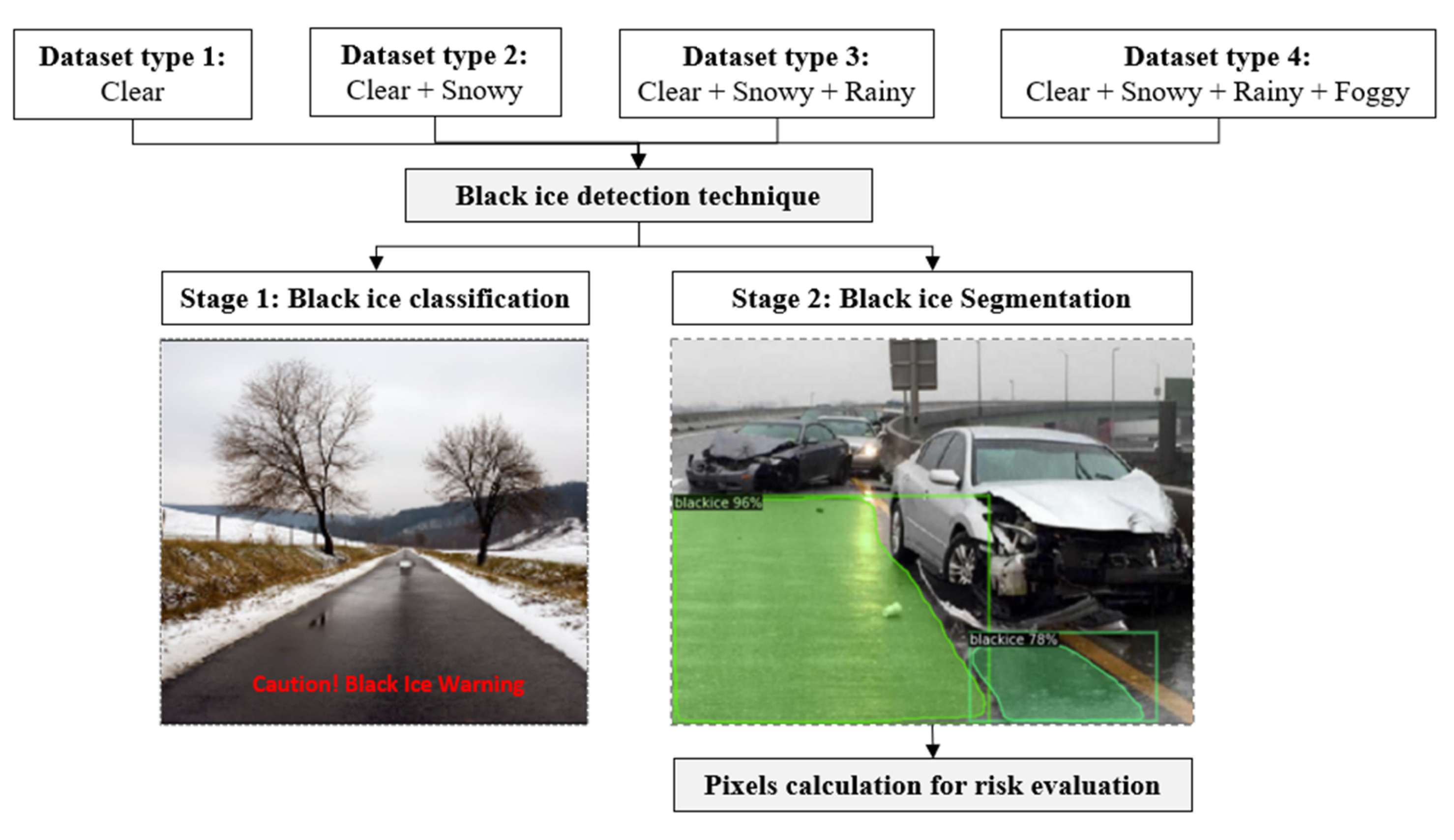
2.1. Overview

The study intends to develop efficient ways to create an adaptable deep-learning approach that may be used in several regions. The image dataset of this study was created using a variety of pavement textures and climate types. The trial dataset harvesting suggested that these circumstances may have a major influence on the effectiveness of black ice detection. Additionally, the conventional bounding box for black ice monitoring only generates anchor boxes, which may not be sufficient to accurately compute and evaluate the volume of black ice. Therefore, this study uses cutting-edge image segmentation technology to accurately determine the black ice zone volume. The research flowchart is presented in Figure 1.

2.2. Dataset Preparation

2.2.1. Data Collecting and Pre-Processing

In this research, the training dataset was generated by gathering unprocessed pictures via the online platform, in-person highway inspections, and Google Street View to obtain training images within a broad range of potential circumstances. Two distinct kinds of pavement and the diversity of meteorological circumstances were used to construct the dataset. Photo resolutions varied between recorder devices from 360p to 720p. The datasets were controlled to share equivalent distributions across weather, lighting, and traffic conditions to ensure quality. The dimensions of the polygons formed within the border of the black ice pattern were preserved in the JavaScript Object Notation (JSON) files that were created from the labeled photos. Recognition of black ice patterns is based on the Korean pavement survey expert and suggestions from related black ice research [32]. By applying the MATLAB Image Labeler program, 800 photos have been physically classified with the labels “Back ice” and “Safety,” respectively. Both conditions were designed to share the equivalent number of photos of 400 to ensure the stability of the training process. Examples of the gathered raw photos used to create the data source are shown in Figure 2. The dataset’s COCO format is constituted of a JSON file that includes all of a picture’s details, including size, annotations, and labels of its polygons bounding.

Table 1. Summary of dataset composition (number of photos).

Pavement Types	Weather Types	Train Data	Validation Data	Test Data	Total
Asphalt pavement	Clear	128	16	16	160
	Snow	128	16	16	160
	Rainy	128	16	16	160
	Foggy	128	16	16	160
Concrete pavement	Clear	128	16	16	160
Total		640	80	80	800

provides a summary of the dataset’s categorization.

2.2.2. Data Labelling

The dimensions of the polygons formed within the border of the black ice pattern were preserved in the JavaScript Object Notation (JSON) files that were created from the labeled photos. Recognition of black ice patterns is based on the Korean pavement survey expert and suggestions from related black ice research [32]. By applying the MATLAB Image Labeler program, 800 photos have been physically classified with the labels “Back ice” and “Safety,” respectively. Both conditions were designed to share the equivalent number of photos of 400 to ensure the stability of the training process. Examples of the gathered raw photos used to create the data source are shown in Figure 2. The dataset’s COCO format is constituted of a JSON file that includes all of a picture’s details, including size, annotations, and labels of its polygon bounding.

2.2.3. Adjustment of Brightness

In the trial training process, the results indicated that the white color may be identical to the glossy/flashlight of black ice pattern on the pavement. The initial works on this research reveal that lowering the brightness of concrete pavement to the optimized value may significantly improve the detection effectiveness. It can be attributed to the reduced bright color/white appearance of concrete.

Considering the process of adjusting brightness in images, the boundary value of 1.0 is significant because it determines how bright or dark objects appear in the image. When using Keras, a value of 1.0 is considered neutral and represents the original image’s threshold between brightness and darkness, so it has no effect on the image. A value lower than 1.0, such as 0.3 to 0.8, makes the image darker, while a value higher than 1.0, such as 1.1 to 1.8, makes it brighter. The research being discussed subjected concrete photos to a brightness value between 0.1 and 0.2, as shown in Figure 3.

2.2.4. Data Augmentation

Enlarging the dataset is vital for generating data diversity, since there are limitations on high-quality photos of black ice presently. As a result, the ImageDataGenerator tool was used to generate and enhance collected photos. Additionally, the research did not concentrate on a particular climate type, but rather attempted to equalize the number of weathers. Thus, several augmentation approaches for various climate conditions were applied. The augmentation procedures involved some well known methods by utilizing the suggested packages [33], ranging from positional augmentation (random flipping, scaling, rotating, cropping, and padding) to color augmentation to improve the diversity of black ice on pavements (random contrast, saturation). The majority of the augmentation methods used a random probability of 0.5. In the image classification process, all of the photos were cropped to 300 × 300 pixel resolution to minimize the processing cost and training time [24]. Likewise, the output images also share the equivalent resolution. Besides, the sizes from 200 to 600 having a 100 increment were used as properties for resizing technique.

Afterward, training data made up 80% of the enhanced data, while testing and validation data made up the remaining 20%. A large increase in the training iteration for convergence may result from the over-augmentation process, according to findings from related research [24]. The effectiveness of the augmentation technique was therefore examined in this research. By employing enhanced data, the model utilizing the proposed architecture was built.

2.3. Deep Learning-Based Object Detection

Based on a customized version of the Mask R-CNN architecture [34], the constructed automatic black ice segmentation process is shown in Figure 4. To be discussed subsequently in this research, the core design of the original Mask R-CNN architecture was adjusted to make it more effective for identifying black ice. The enhanced Mask R-CNN was fed with annotated training and validation images for the training and validation processes based on a suggestion from previous research [35]. There are two basic phases in the design of the bounding box for black ice detection via Mask R-CNN. Initially, several bounding boxes were paired with probabilities (Figure 5A). The label of the object is then generated by refining the best bounding box (Figure 5B,C). Currently, the majority of effective object detection and classification methods developed on the Mask R-CNN employ this method [28]. Therefore, the proposed research employs this model to address the black ice detection difficulty. Rather than creating a new Mask R-CNN network, this research employs a modern object detection technique that has been implemented in Detectron2 [36] to shorten the building process. In this image segmentation process, Detectron2 was incorporated to utilize its state-of-the-art pre-trained model. Detectron2 was initially trained using photos of real-world items rather than specific forms such as a black ice pattern. Detectron2 supports transfer learning to train an object identification network with a unique dataset from a different domain. Faster R-CNN, Mask R-CNN, RetinaNet, and DensePose are cutting-edge object identification methods that are well executed in the Detectron2 framework. Three convolutional blocks, each with a max pooling layer, were added to a sequential model developed in the deep learning toolkit Keras [37].

2.3.1. Conventional Faster R-CNN

In the conventional Image Segmentation process, the Faster R-CNN model was developed from three main components, including the Backbone network, Region network, and Box Head. The properties of the input image were first extracted from the Backbone. They were then transferred to the Region network to detect the object. After which, the box identification and bounding box localization were predicted through the Box Head zone. The modeling of Faster R-CNN is shown in the following Figure 6. Besides, a significant innovation in this network is batch normalization. It enables quicker and greater consistent learning by stabilizing the data dispersion from one layer before transmitting it to another. By preventing disappearing gradients, the approach further facilitates gradient descent.

2.3.2. Mask R-CNN

The Mask R-CNN is founded on the Faster R-CNN methodology, which incorporates an additional object mask as an output. Improved accuracy in object detection and photo segmentation is accomplished by the class label applied to the object mask and the bounding box specifying the region [34]. Mask R-CNN incorporates a component for predicting segmentation masks for each region of interest (RoI). In the next phase, RoIAlign performs the function of the ROI pool that assists in keeping spatial features that the ROI pool misaligns. A fixed-size feature map is produced using RoIAlign with binary interpolation. After that, the output of the RoIAlign layer is passed through the Mask head. Subsequently, it produces a mask for each RoI, segmenting a picture pixel-by-pixel. The Mask R-CNN structure is illustrated in Figure 7.

Although slight customization of the Mask R-CNN model was performed by tuning up some hyper-parameters, the default configuration of the pre-trained model was maintained in this study. Numerous equivalent base models are offered by Detectron2 [36].

Furthermore, R101-FPN1, FP50, and X101-FPN are three recent frequently applied models in Mask R-CNN. When compared to other models, they exhibit superior Mask R-CNN box Average Precision (AP). Even when R101-FPN outperforms the ImageNet benchmark in terms of box AP [24], it requires more time to train and estimate and occasionally exhibits overfitting. Therefore, this research also incorporates three models for detection performance comparison.

2.3.3. Improved Mask R-CNN

In this research, Mask R-CNN was improved by using ResNetV2 as the core framework to optimize the detection accuracy and training time [35]. Before activating the convolution, batch normalization (BN) and rectified linear units (ReLU) were implemented in ResNetV2 to improve the residual connectivity of the network [38]. The proposed ResNetv2-based architecture was initiated using pre-trained weights from the Mask R-CNN recognition model, which reduced a significant amount of training expenses. The fundamental design of ResNetV2 is shown in Figure 8, which includes batch normalization as the first step, followed by an activation algorithm, as well as weight updates thereafter. Afterward, the batch normalization was carried out followed by the ReLU activation function, and the weights were optimized. In this ResNetv2 model, pre-activation of the weight layers is the distinguishing feature, as opposed to conventional post-activation [38]. Overall, the performance of the system was significantly enhanced by such changes.

Besides, further steps involving the data normalization procedure were implemented to minimize data leaking during the hyperparameter optimization phase. The stochastic gradient descent (SGD) approach incorporating momentum has been chosen through this work to reduce the cross-entropy loss throughout the training stage. By modifying the connection weights and improving precision, this iterative process minimized the loss. Transfer learning of previously trained models on the ImageNet database has been utilized to determine the best structure for the monitoring objective condition. Without taking into account stochastic initialization weights from the beginning, the transmission of acquired generic features enabled greater efficiency and fewer trained costs. On the other hand, the base model’s predictions of the high-level properties of the new dataset are improved by the tuning of hidden layers, as well as the additional classified layer.

2.3.4. Applications

In this research, the coding process was performed by using Python coding. On Google Colab, all deep learning networks in this research were developed on a Nvidia Tesla P100/K80/T4 GPU. TensorFlow, an open application framework for dataflow programming, and Keras, an open-source neural network library in Python, were applied to develop the Mask R-CNN for black ice detection. A pre-trained model using the Common Objects in Context (COCO) was used to train on the black ice dataset.

2.3.5. Hyperparameters

The network hyperparameters must be established before the training phase. This process was developed after the network structures and the dataset had been determined. Since these parameters are independent of the networks, they could only be determined through heuristics rather than through direct dataset estimation. The Mask R-CNN network has a lot of adjusted hyperparameters when being trained. The related study suggests that exploring all alternative setups would be extremely time and resource-intensive [24]. Therefore, the Mask R-CNN in this research mostly utilizes the default settings. The research purposely defined the class numbers as 2 (black ice zone vs. safe zone).

The normal settings from Detectron2 were preserved for all subsequent setups. The accessible hyperparameter tuning toolkit Optuna [39] was employed to adjust the model parameters, including the learning algorithm. Hyperparameter configuration for Mask R-CNN is presented in

Table 2. Hyperparameters configuration for Mask R-CNN.

Model Parameter	Value
cfg.SOLVER.BASE_LR (Base learning rate)	0.00025
cfg.SOLVER.IMS_PER_BATCH (Images per batch)	4
cfg.SOLVER.GAMMA (Decreases learning rate over time)	0.05
cfg.SOLVER.MAX_ITER (No. of iterations)	2000
cfg.MODEL.ROI_HEADS.BATCH_SIZE_PER_IMAGE (No. of regions of interest)	16
cfg.MODEL.ROI_HEADS.NUM_CLASSES (No. of classes)	2
cfg.MODEL.ROI_HEADS.SCORE_THRESH_TEST (Parameter to balance recall/precision)	0.5

. Based on trial experiments, an initial set amount of ten iterations, a small-batch capacity of four photos, a momentum of 0.8, and a regularization of 0.0001 have all been taken into consideration when determining the optimized network hyperparameters. These numbers have been explored for the network’s training procedure to determine an appropriate beginning learning rate of 0.00025.

2.4. Comparable Architectures

The YOLO family of algorithms is widely used for object detection in civil engineering, allowing for improved safety and maintenance of infrastructure. Recent developments include YOLOv6 [20,40], v7 [21], and v8 [22], which have found applications in structural monitoring and safety, such as detecting cracks in concrete structures and monitoring the movement of vehicles and pedestrians in construction sites. It is worth noting that, while the YOLO family of algorithms has seen several recent developments, the conventional YOLOv4 model remains a highly effective solution for object detection [41]. YOLOv4 was released in 2020 and has achieved state-of-the-art performance on multiple benchmarks, including COCO, PASCAL VOC, and KITTI [41]. In addition, YOLOv4 is highly efficient and can run in real-time on a standard GPU, making it a practical solution for many applications. Its architecture includes several advanced features, such as spatial pyramid pooling, a path aggregation network, and a novel loss function that improve its detection accuracy and robustness. Overall, while YOLOv6, v7, and v8 offer exciting new features and improvements, the conventional YOLOv4 model remains a highly effective and efficient solution for object detection in civil engineering and other fields.

In addition to the proposed Mask R-CNN architecture, the research also incorporated popular training models, including Yolov4 [41], Yolov4-ResNet50 [41,42], and Yolov4-Tiny [43] for comparison purposes. The calibration and tuning process of these architectures were based on the defaulted values considering the developed Mask R-CNN hyperparameters and the final hyperparameters of the comparable models. These are summarized in

Table 3. Hyperparameter configuration of comparable architectures.

Model	Width × Height	Momentum	Decay	Learning Rate	Activation
Yolov4	300 × 300	0.9	0.00005	0.0013	Leaky ReLU
Yolov4-Tiny	300 × 300	0.85	0.0005	0.0025	Leaky ReLU
Yolov4-ResNet50	300 × 300	0.85	0.0005	0.0002	Leaky ReLU

.

2.5. Comparative Analysis and Evaluation

A comparative analysis based on the percentage of correctly identified pixels is described below:

$$GA=\frac{TP+TN}{TP+TN+FP+FN}$$

(1)

where: GA = global accuracy; TP = true positives; TN = true negatives; FP = false positives, and FN = false negatives.

In order to optimize and build the capabilities of the segmentation structure, the precision and intersection-over-union (IoU) scores were incorporated for each class. The overlap and union between the projected segmentation and the actual segmentation constitute the IoU measure (Equation (2)).

$$IoU=\frac{TP}{TP+FP+FN}$$

(2)

It was considered that there was no intended class when the probability of the output was below the criterion of 0.5. If the identification is a true positive, it is determined by comparing the recognition rate to the actual data. At least 50% of the IoU score of the identified bounding box must be obtained to meet the research target.

Cross-Entropy Loss Function

In this research, the cross-entropy loss function treats background and black ice pixels equally, which makes it unsuitable for a dataset with uneven samples of black ice. To address this, a weighted binary cross-entropy loss function can be used instead, as shown in Equation (3), which assigns different weights to the different types of pixels [44,45].

$$Weighted binary cross-entropy\left(W,w^{\left(m\right)}\right)=-\beta {\displaystyle \sum }_{iϵY_{+}}log{P}_i\left(y_i=1|X;W,w^{\left(m\right)}\right)-\left(1-\beta \right){\displaystyle \sum }_{iϵY_{-}}log{P}_i\left(y_i=0|X;W,w^{\left(m\right)}\right)$$

(3)

During image-to-image training, the loss function is calculated for every pixel in the training image, $X=(x_i, i=1,\dots ,\left|X\right|$) and black ice map $Y=(y_i, i=1,\dots ,\left|Y\right|$). Based on $\left(y_i|X;W,w^{\left(m\right)}\right)= \sigma \left(a_i^m\right)ϵ\left[\left(0,1\right)\right]$, a sigmoid function σ is used to calculate the value of weight β based on the activation at each pixel. This helps to address any imbalance between black ice and non-black ice pixels, which can be further adjusted artificially. This $\beta =\left|Y_{-}\right|/Y$ and $1-\beta =\left|Y_{+}\right|/Y$ refers to the ratio of black ice and non-black ice pixels present in the ground truth image.

3. Results and Discussions

3.1. Black Ice Classification

The training performance of the proposed black ice classification model is presented in Figure 9 and

Table 4. The average precision measured from each type of dataset (black ice classification).

No.	Machine Learning Methods	Pavement Types	Precision
			Weather Data Type
			1st Cond.	2nd Cond.	3rd Cond.	4th Cond.
			Clear	Clear, Snowy	Clear, Snowy, Rainy	Clear, Snowy, Rainy, Foggy
1	Image classification	Asphalt pavement	95.6%	93.3%	82.1%	63.5%
2	Image classification	Concrete pavement	94.2%	85.4%	78.8%	58.1%

. In general, it can be noted that black ice can be detected by applying a convolution neural network. The training total loss greatly drop from approximately 1.6 to 0.4 within the initial 50 epochs, then the loss gradually reduced from 0.4 to 0.2 in the following 100 epochs. The total loss reduction slightly decreases in the remained epochs and converges after 400 epochs. Regarding the impact of weather, the detection effectiveness varied between multiple pavements and weather types. The test results reveal that the precision of the learning depends significantly on the constitution of weather types. The increase in the number of weathers leads to a drop in the precision of the training.

Adding Foggy weather photos into the dataset especially led to a great drop in precision. This may be attributed to the characteristic of the Foggy pavement surface texture, which has an identical pattern to black ice (glossy pattern, etc.), cultivating the reduction in the training performance. Besides, the addition of concrete pavement photos leads to a slight drop in the model precision. In general, the application of CNN has potential for the black ice classification process. The suggested approach is effective for on-site black ice monitoring, since it is adaptable to a variety of pavement surfaces and weather. Nevertheless, the diverse climates and pavement types may result in inaccuracy in the detection model.

3.2. Black-Ice Segmentations

3.2.1. Overall Results

As illustrated in Figure 10, the findings confirm that it is feasible to detect black ice on pavement via the image segmentation technique. The developed black ice detection model via Mask R-CNN shows acceptable results, since it can distinguish black ice and safe pavement (Figure 11a). In addition, the accuracy score significantly decreases on wet and glossy pavement, especially when surrounded by fog or snow as shown in Figure 11b.

In general, the type of surface and the climate are considered to be extremely important factors in the detection performance. For instance, if the pavement is a concrete type, the mask of the detection may be inaccurate due to the white color of the concrete pavement. In other words, this color may be identical to the glossy/flashlight of the black ice pattern. The training results also reveal that the influence of pavement type will become severe under combined weather conditions, especially in rainy and foggy conditions. This issue will be discussed in the following section.

3.2.2. Effect of Weather on Training Performance

Figure 12 illustrates the training loss and training accuracy concerning the weather-type conditions. In general, the proposed black ice detection model achieved reasonable performance scores. It is possible to use the mask-RCNN as the object-detection model, since the training results reveal that the overall total loss is less than 0.3, and the accuracy is higher than 0.9. The convergence of the model can be obtained after 2000 iterations, except for the 4th condition, constituting all types of weather. Additional training for the 4th condition suggests that the largest dataset can be converged after 3000 iterations.

Considering the impact of the weather dataset, the training score indicates that the increase in the climate dataset leads to a degradation in the training performance. These results agree with the findings from the previous image classification step, since adding the Foggy type causes a great drop in accuracy. As can be seen from Figure 12a, there is an obvious gap between the 1st condition with only “Clear” data and the 4th condition having all climate types (Clear, Snowy, Rainy, and Foggy). Therefore, it can be concluded that weather characteristics noticeably contribute to the training effectiveness of the object detection model. It can be explained by the similarity of the photo’s attributes of black ice (color, brightness, texture) towards frost and wet pavement during rainy and foggy conditions. Additionally, based on the test datasets analysis, the results confirm the appropriate functioning of the model when all testing groups passed the Mask-R-CNN accuracy of higher than 80%. In general, although there is a slight gap between the training dataset and the test dataset, since the accuracy of the testing dataset is 5–15% lower than that of the testing dataset, the impacts of diversified environmental conditions still maintain across all scenarios.

The results reveal the validity of this approach for the automated evaluation of black ice on pavements, notwithstanding some small inaccuracies. Accordingly, there are occasional errors detected concerning climate conditions. The distinctive inaccurate detection warns about the size of black ice having more than the actual value. Thus, a greater training set may enhance the adaptability and capability of the classifier for potential uses. Besides, to obtain increased efficiency, an extensive assessment of the best model parameters was carried out. The loss function was reduced while taking into account a training procedure with iterations on a mini-batch size of 4 to monitor the full converging performance and prevent overfitting. The ultimate set of optimized model parameters is as follows: regularization of 0.0001, a momentum of 0.8, a learning rate of 0.00025, and a mini-batch size of 4.

3.2.3. Average Precision Results AP50

The black ice segmentation precision is summarized in

Table 5. The average precision at IOU = 0.5 (AP50).

			AP50: The Average Precision at IOU = 0.5
No.	Machine Learning Methods	Pavement Types	Combined Weather Data
			1st Cond.	2nd Cond.	3rd Cond.	4th Cond.
			Clear	Clear, Snowy	Clear, Snowy, Rainy	Clear, Snowy, Rainy, Foggy
1	Image segmentation (R101-FPN Model)	Asphalt pavement	92.5%	83.7%	75.3%	54.6%
2	Image segmentation (R101-FPN Model)	Asphalt pavement and Concrete pavement	89.1%	80.3%	72.8%	48.5%

. In this context, the findings demonstrate that the 4th condition has the lowest precision among the four categories, while “Clear conditions” has the best value. For example, the precision AP50 (average precision at IOU = 0.5) of the 1st, 2nd, 3rd, and 4th conditions are 92.5%, 83.7%, 75.3%, and 54.6%, respectively. The AP50 results indicate that the black ice detection technique via image segmentation may suffer from diverse meteorological conditions. Besides, the addition of concrete pavement also cultivates the variation in the precision of the trained model. The “white” color of concrete pavement may lead to inaccuracy during learning. This can be explained by how the segmentation perceives black ice as a flashy or glossy pattern formed on top of pavements. The white pattern on the concrete pavement may be mistakenly detected as black ice in the training process. From a perceptual perspective, these findings concern how challenging it is to identify black ice in real-world scenarios.

3.2.4. Pre-Trained Model Evaluation

The performance metrics in Figure 13 illustrate the comparative assessment of deep learning models. Overall, it can be seen from the accuracy indication that the training results were relatively similar between models. The result demonstrates that, in the first 500 iterations, the train dataset’s accuracy increased significantly. Afterward, the training accuracy slightly achieves the convergence stage. The efficiency of the train results has been marginally increased by adjustments to the pre-trained model. The trained results demonstrate that the efficiency gap between the three image segmentation models can be ignored. The final average accuracy score was 97%, demonstrating the adaptability of the learning effectiveness for predicting black ice.

Considering the training time, which is very essential in real-time detection, as shown in

Table 6. Summary of comparison between different Image segmentation models.

	Image Segmentation Model
	FP50	R101-FPN	X101-FPN
Required time per iteration (second)	0.87	0.83	1.43
Iteration to convergence	2200	1800	2700

, the results also indicate that model R101-FPN required the shortest amount of time to train the dataset when compared to the other models. For example, while the X101-FPN models might take up to 1.43 s to train one iteration, the R101-FPN models took only 0.83 s. The number of iterations for convergence is also higher in the method trained by the former. Additionally, using the multiple augmentation approach significantly lengthens the training period. The training process also shows that it requires a significant amount of time to achieve the required convergence.

3.3. Architecture Comparison

Table 7. Performance results between different architectures.

	Image Segmentation Model
	Mask R-CNN	Yolov4	Yolov4-Tiny	Yolov4-ResNet50
Required time per iteration (second)	0.83	0.65	0.53	0.78
AP50 on clear weather (asphalt pavement)	92.5%	81.3%	73.7%	84.9%

summarizes the performance between different architectures using the equivalent dataset for black ice recognition. The results reveal that Yolov4-tiny achieved the fastest training time among different structures, followed by Yolov4 and Yolov4-ResNet50. However, it should be noted that the fastest training model also accounted for the lowest training precision, since the AP50 precision of this architecture was only 73.7%. Meanwhile, although the Mask R-CNN may require a longer processing time of 0.83 secs per iteration, this architecture outperforms the other models in the AP50 scale, which achieved the highest value of 92.5%, suggesting the practical application for black ice warning. In general, the evaluation results show that the proposed Mask R-CNN model outperforms the other models in terms of accuracy. However, the inference time of the Mask R-CNN model is slower than the YOLO models. While the Mask R-CNN model achieves higher accuracy than the YOLO models, it is unclear whether the YOLO models can be further improved by fine-tuning. Therefore, the additional analysis should be performed in the next stage of this research to investigate the possibility of improving the YOLO models with fine-tuning. This analysis will help to clarify the strengths and limitations of each of these models and enable researchers to choose the most appropriate model for their specific use case. These findings contribute to the ongoing efforts to develop efficient and accurate object detection models for a wide range of applications.

3.4. Risk Assessment

Once the black ice danger has been identified, it is feasible to retrieve the segmentation zone to assess the black ice risk under practical circumstances. In addition to automating the detection, the suggested deep learning-based monitoring technique also extracts essential data to analyze the risk percentage of black ice. By utilizing the MATLAB code, the photo area attributes can be generated after each pixel class has been determined. An analysis made on the test pictures in Figure 14 linked to the precise number of pixels in the “Black Ice” and “Pavement Background” regions is shown in

Table 8. Pixel calculation on test photos.

	Black Ice Zone [Pixel]	Pavement Background [Pixel]	Black Ice Risk (%)
Figure 14A	1,634,750	2,053,652	79.60
Figure 14B	758,552	1,803,374	42.06
Figure 14C	2,412,763	2,697,551	89.44

. The number (%) shown in the photos indicates the probability of black ice. Additionally, with the right spatial calibrating parameter, the degree of danger can be expressed as a percent of the entire region. The degree of black ice risk is currently being developed in mobile apps for traffic users to support the purpose of safe driving.

3.5. The Effect of Augmentations

In general, after applying multiple standard augmentation methods, the designed networks did not execute much superiority and the learning iterations required more repetitions to converge. In particular,

Table 9. Summary of the augmentation methods on the detection efficiency.

No.	Augmentation Methods	Image Classification	Image Segmentation
			X101-FPN	FP50	R101-FPN
1	Cutoff	$+$15.6%	$-$21.2%	$-$18.7%	$-$22.6%
2	Random contrast	$+$5.6%	$-$11.3%	$-$5.1%	$-$7.3%
3	Cropping	$-$9.2%	$-$18.5%	$-$16.1%	$-$16.0%
4	Flipping	$+$4.7%	$+$2.7%	$+$2.1%	$+$2.9%
5	Scaling	$-$3.1%	$-$6.4%	$-$6.1%	$-$5.4%
6	Rotating	$+$2.2%	$+$5.6%	$+$4.9%	$+$5.2%
7	Padding	$+$12.8%	$-$17.5%	$-$22.0%	$-$19.3%
8	Resizing	$+$14.5%	$+$6.7%	$+$5.1%	$+$5.9%

($-$): decrease precision; ($+$): improve precision; The intensity of color indicates the impact of the augmentation, the darker the color, the greater the impact.

demonstrates the comparison of the network using standard augmentations, and extra augmentations including random cutoff, stochastic contrast, and scaling that led to poorer accuracy of results. The Detectron2 Mask R-CNN solution already had constructed dropout layers which may explain why the cutout augmentation approach does not provide enhancement in accuracy. The lack of efficiency improvement from the contrast approach may be due to the training set being comprised already of photos with various lighting factors. In other words, the user already obtained photos with various bright intensity settings. Besides, the failure of the cropping augmentation strategy may be attributable to Mask R-CNN primarily utilizing the ground-truth squares, or areas of interest instead of a full photo [46]. Overall, the application of proper augmentation methods should be concerned to sustain the performance of the training process. Instead of conducting further augmentation approaches, enrichment in the original dataset is recommended.

3.6. Potential Applications

The black ice detection app could be installed on vehicles and drones to provide a solution to warn communities of black ice. Furthermore, users would be capable of anticipating black ice formation by forecasting the phenomenon in line with optimizing the parameters of the deep learning model. Additionally, CCTV is anticipated to play a significant role in C-ITS (Cooperative Intelligent Transport System) within the coming years. This makes it possible to deploy in a favorable region for predicting the probability of black ice.

4. Conclusions

This study proposes a methodology for detecting black ice using a convolutional neural network approach to reduce black ice fatalities. By identifying and defining “Black ice” and “Safe” zones on actual structures at the pixel level, a computerized assessment based on deep learning can be developed. The datasets used in this study were carefully created to ensure a diverse variety of applicability, including pictures gathered through an online platform, in-person highway inspections, and Google Street View in regulated environments. The study took into account various climates and pavement types to create a comprehensive approach suitable for on-field inspections. The following remarks can be found in the study:

• Through the image classification and object detection process, the training results suggest that the “Clear Weather” groups achieved the maximum precision, while the “Combined weather” dataset (Clear, Snow, Rainy, Foggy) is considered the most difficult to identify black ice.
• Weather datasets greatly contribute to the training effectiveness of the deep learning model. For example, the precision AP50 values for the first, second, third, and fourth conditions are 92.5%, 83.7%, 75.3%, and 54.6%, respectively. The image segmentation technique for black ice detection may encounter difficulties in various weather conditions due to the identical textures between the black ice pattern (color, brightness, and texture attributes) and frost/wet pavements during rainy and foggy weather. In addition to the climate condition, concrete pavement can cause inaccuracies in detection due to its white color, making it difficult to distinguish from glossy black ice.
• Among all pre-trained models, the best model image segmentation (R101-FPN) was modified to configure hyperparameters, resulting in a maximum precision of 93.7%. All proposed deep learning models encountered overlapped image segmentation issues due to the limitation of the training dataset.
• By retrieving the segmentation zone, the degree of danger area can be determined by calculating the number of pixels, promoting a potential tool for monitoring the risky percentage of traffic users.
• Although the Mask R-CNN may require a longer processing time of 0.83 secs per iteration, this architecture outperforms the other models (Yolov4) in the AP50 scale, which achieved the highest value of 92.5%, suggesting the practical application for black ice warning.
• Overall, this study reveals that black ice detection via deep learning methods is possible and can supplement the safety of driving during winter. The forthcoming study aims to enhance the segmentation measures by incorporating a bigger dataset and hyperspectral photos that offer more details about each pixel. Additionally, visualizations and inputs from LiDAR sensors would be combined to create a completely computerized monitoring process.

References

- Riehm, M.; Gustavsson, T.; Bogren, J.; Jansson, P.E. Ice Formation Detection on Road Surfaces Using Infrared Thermometry. Cold Reg. Sci. Technol. 2012, 83–84, 71–76. [Google Scholar] [CrossRef]
- Abdelaal, A.; Sarayloo, M.; Nims, D.K.; Mohammadian, B.; Heil, J.; Sojoudi, H. A Flexible Surface-Mountable Sensor for Ice Detection and Non-Destructive Measurement of Liquid Water Content in Snow. Cold Reg. Sci. Technol. 2022, 195, 103469. [Google Scholar] [CrossRef]
- Tabatabai, H.; Aljuboori, M. A Novel Concrete-Based Sensor for Detection of Ice and Water on Roads and Bridges. Sensors 2017, 17, 2912. [Google Scholar] [CrossRef]
- Alimasi, N.; Takahashi, S.; Enomoto, H. Development of a Mobile Optical System to Detect Road-Freezing Conditions. Bull. Glaciol. Res. 2012, 30, 41–51. [Google Scholar] [CrossRef]
- Abdalla, Y.E.; Iqbal, M.T.; Shehata, M. Black Ice Detection System Using Kinect. In Proceedings of the 2017 IEEE 30th Canadian Conference on Electrical and Computer Engineering (CCECE), Windsor, ON, Canada, 30 April–3 May 2017. [Google Scholar] [CrossRef]
- Minullin, R.G.; Mustafin, R.G.; Piskovatskii, Y.V.; Vedernikov, S.G.; Lavrent’Ev, I.S. A Detection Technique for Black Ice and Frost Depositions on Wires of a Power Transmission Line by Location Sounding. Russ. Electr. Eng. 2011, 82, 541–543. [Google Scholar] [CrossRef]
- Gailius, D.; Jacenas, S. Ice Detection on a Road by Analyzing Tire to Road Friction Ultrasonic Noise. Ultragarsas 2007, 62, 17–20. [Google Scholar]
- Ma, X.; Ruan, C. Method for Black Ice Detection on Roads Using Tri-Wavelength Backscattering Measurements. Appl. Opt. 2020, 59, 7242. [Google Scholar] [CrossRef]
- Shen, Y.; Yu, Z.; Li, C.; Zhao, C.; Sun, Z. Automated Detection for Concrete Surface Cracks Based on Deeplabv3+ BDF. Buildings 2023, 13, 118. [Google Scholar] [CrossRef]
- Haruehansapong, K.; Roungprom, W.; Kliangkhlao, M.; Yeranee, K.; Sahoh, B. Deep Learning-Driven Automated Fault Detection and Diagnostics Based on a Contextual Environment: A Case Study of HVAC System. Buildings 2023, 13, 27. [Google Scholar] [CrossRef]
- Dong, C.Z.; Catbas, F.N. A Review of Computer Vision–Based Structural Health Monitoring at Local and Global Levels. Struct. Heal. Monit. 2021, 20, 692–743. [Google Scholar] [CrossRef]
- Spencer, B.F.; Hoskere, V.; Narazaki, Y. Advances in Computer Vision-Based Civil Infrastructure Inspection and Monitoring. Engineering 2019, 5, 199–222. [Google Scholar] [CrossRef]
- Ramanna, S.; Sengoz, C.; Kehler, S.; Pham, D. Near Real-Time Map Building with Multi-Class Image Set Labeling and Classification of Road Conditions Using Convolutional Neural Networks. Appl. Artif. Intell. 2021, 35, 803–833. [Google Scholar] [CrossRef]
- Xie, Q.; Kwon, T.J. Development of a Highly Transferable Urban Winter Road Surface Classification Model: A Deep Learning Approach. Transp. Res. Rec. J. Transp. Res. Board 2022, 2676, 445–459. [Google Scholar] [CrossRef]
- Que, Y.; Dai, Y.; Ji, X.; Kwan Leung, A.; Chen, Z.; Tang, Y.; Jiang, Z. Automatic Classification of Asphalt Pavement Cracks Using a Novel Integrated Generative Adversarial Networks and Improved VGG Model. Eng. Struct. 2023, 277, 115406. [Google Scholar] [CrossRef]
- Tang, Y.; Huang, Z.; Chen, Z.; Chen, M.; Zhou, H.; Zhang, H.; Sun, J. Novel Visual Crack Width Measurement Based on Backbone Double-Scale Features for Improved Detection Automation. Eng. Struct. 2023, 274, 115158. [Google Scholar] [CrossRef]
- Zhang, J.; Qian, S.; Tan, C. Automated Bridge Surface Crack Detection and Segmentation Using Computer Vision-Based Deep Learning Model. Eng. Appl. Artif. Intell. 2022, 115, 105225. [Google Scholar] [CrossRef]
- Pei, L.; Sun, Z.; Xiao, L.; Li, W.; Sun, J.; Zhang, H. Virtual Generation of Pavement Crack Images Based on Improved Deep Convolutional Generative Adversarial Network. Eng. Appl. Artif. Intell. 2021, 104, 104376. [Google Scholar] [CrossRef]
- Ali, R.; Chuah, J.H.; Talip, M.S.A.; Mokhtar, N.; Shoaib, M.A. Crack Segmentation Network Using Additive Attention Gate—CSN-II. Eng. Appl. Artif. Intell. 2022, 114, 105130. [Google Scholar] [CrossRef]
- Li, C.; Li, L.; Jiang, H.; Weng, K.; Geng, Y.; Li, L.; Ke, Z.; Li, Q.; Cheng, M.; Nie, W.; et al. YOLOv6: A Single-Stage Object Detection Framework for Industrial Applications. arXiv 2022, arXiv:2209.02976. [Google Scholar]
- Wang, C.-Y.; Bochkovskiy, A.; Liao, H.-Y.M. YOLOv7: Trainable Bag-of-Freebies Sets New State-of-the-Art for Real-Time Object Detectors. arXiv 2022, arXiv:2207.02696. [Google Scholar]
- Chaurasia, A.; Qiu, J. YOLO by Ultralytics. Available online: https://docs.ultralytics.com/ (accessed on 5 March 2023).
- Khan, M.N.; Ahmed, M.M. Weather and Surface Condition Detection Based on Road-Side Webcams: Application of Pre-Trained Convolutional Neural Network. Int. J. Transp. Sci. Technol. 2022, 11, 468–483. [Google Scholar] [CrossRef]
- Pham, V.; Pham, C.; Dang, T. Road Damage Detection and Classification with Detectron2 and Faster R-CNN. In Proceedings of the 2020 IEEE International Conference on Big Data, Atlanta, GA, USA, 10–13 December 2020; pp. 5592–5601. [Google Scholar] [CrossRef]
- Singh, J.; Shekhar, S. Road Damage Detection and Classification in Smartphone Captured Images Using Mask R-CNN. arXiv 2018, arXiv:1811.04535. [Google Scholar]
- Chen, J.; Li, A.; Bao, C.; Dai, Y.; Liu, M.; Lin, Z.; Niu, F.; Zhou, T. A Deep Learning Forecasting Method for Frost Heave Deformation of High-Speed Railway Subgrade. Cold Reg. Sci. Technol. 2021, 185, 103265. [Google Scholar] [CrossRef]
- Chen, W.; Luo, Q.; Liu, J.; Wang, T.; Wang, L. Modeling of Frozen Soil-Structure Interface Shear Behavior by Supervised Deep Learning. Cold Reg. Sci. Technol. 2022, 200, 103589. [Google Scholar] [CrossRef]
- Ansari, S.; Rennie, C.D.; Clark, S.P.; Seidou, O. IceMaskNet: River Ice Detection and Characterization Using Deep Learning Algorithms Applied to Aerial Photography. Cold Reg. Sci. Technol. 2021, 189, 103324. [Google Scholar] [CrossRef]
- Patel, T.; Guo, B.H.W.; van der Walt, J.D.; Zou, Y. Effective Motion Sensors and Deep Learning Techniques for Unmanned Ground Vehicle (UGV)-Based Automated Pavement Layer Change Detection in Road Construction. Buildings 2023, 13, 5. [Google Scholar] [CrossRef]
- Chen, C.; Gu, H.; Lian, S.; Zhao, Y.; Xiao, B. Investigation of Edge Computing in Computer Vision-Based Construction Resource Detection. Buildings 2022, 12, 2167. [Google Scholar] [CrossRef]
- Kim, J.; Kim, E.; Kim, D. A Black Ice Detection Method Based on 1-Dimensional CNN Using MmWave Sensor Backscattering. Remote Sens. 2022, 14, 5252. [Google Scholar] [CrossRef]
- Lee, H.; Kang, M.; Song, J.; Hwang, K. The Detection of Black Ice Accidents for Preventative Automated Vehicles Using Convolutional Neural Networks. Electronics 2020, 9, 2178. [Google Scholar] [CrossRef]
- Buslaev, A.; Iglovikov, V.I.; Khvedchenya, E.; Parinov, A.; Druzhinin, M.; Kalinin, A.A. Albumentations: Fast and Flexible Image Augmentations. Information 2020, 11, 125. [Google Scholar] [CrossRef]
- He, K.; Gkioxari, G.; Dollár, P.; Girshick, R. Mask R-CNN. In Proceedings of the 2017 IEEE International Conference on Computer Vision, Venice, Italy, 22–29 October 2017. [Google Scholar]
- Lee, S.Y.; Le, T.H.M.; Kim, Y.M. Prediction and Detection of Potholes in Urban Roads: Machine Learning and Deep Learning Based Image Segmentation Approaches. Dev. Built Environ. 2023, 13, 100109. [Google Scholar] [CrossRef]
- Wu, Y.; Kirillov, A.; Massa, F.; Lo, W.-Y.R.G. Detectron2. Available online: https://github.com/facebookresearch/detectron2 (accessed on 5 March 2023).
- Keras, F.C. 2015. Available online: https://Keras.Io. (accessed on 5 March 2023).
- He, K.; Zhang, X.; Ren, S.; Sun, J. Deep Residual Learning for Image Recognition. In Proceedings of the IEEE Computer Society Conference on Computer Vision and Pattern Recognition (CVPR), Las Vegas, NV, USA, 27–30 June 2016; pp. 770–778. [Google Scholar] [CrossRef]
- Akiba, T.; Sano, S.; Yanase, T.; Ohta, T.; Koyama, M. Optuna: A Next-Generation Hyperparameter Optimization Framework. In Proceedings of the 25th ACM SIGKDD International Conference on Knowledge Discovery & Data Mining, Anchorage, AK, USA, 4–8 August 2019; pp. 2623–2631. [Google Scholar] [CrossRef]
- Li, C.; Li, L.; Geng, Y.; Jiang, H.; Cheng, M.; Zhang, B.; Ke, Z.; Xu, X.; Chu, X. YOLOv6 v3.0: A Full-Scale Reloading. arXiv 2023, arXiv:2301.05586. [Google Scholar]
- Bochkovskiy, A.; Wang, C.-Y.; Liao, H.-Y.M. YOLOv4: Optimal Speed and Accuracy of Object Detection. arXiv 2020, arXiv:2004.10934. [Google Scholar]
- He, K.; Zhang, X.; Ren, S.; Sun, J. Spatial Pyramid Pooling in Deep Convolutional Networks for Visual Recognition. In European Conference on Computer Vision; Lecture Notes in Computer Science (including subseries Lecture Notes in Artificial Intelligence and Lecture Notes in Bioinformatics); Springer: Cham, Switzerland, 2014; Volume 8691, pp. 346–361. [Google Scholar] [CrossRef]
- Wang, C.Y.; Bochkovskiy, A.; Liao, H.Y.M. Scaled-Yolov4: Scaling Cross Stage Partial Network. In Proceedings of the 2021 IEEE/CVF Conference on Computer Vision and Pattern Recognition (CVPR), Nashville, TN, USA, 20–25 June 2021; pp. 13024–13033. [Google Scholar] [CrossRef]
- Nar, K.; Ocal, O.; Sastry, S.S.; Ramchandran, K. Cross-Entropy Loss and Low-Rank Features Have Responsibility for Adversarial Examples. arXiv 2019, arXiv:1901.08360. [Google Scholar]
- Zhang, Z.; Sabuncu, M.R. Generalized Cross Entropy Loss for Noisy Labels. Adv. Neural Inf. Process. Syst. 2018, 31. [Google Scholar]
- Alfarrarjeh, A.; Trivedi, D.; Kim, S.H.; Shahabi, C. A Deep Learning Approach for Road Damage Detection from Smartphone Images. In Proceedings of the 2018 IEEE International Conference on Big Data (Big Data), Seattle, WA, USA, 10–13 December 2018; pp. 5201–5204. [Google Scholar] [CrossRef]