
Evaluation of the Impact of Input-Data Resolution on Building-Energy Simulation Accuracy and Computational Load—A Case Study of a Low-Rise Office Building
 ,
,
Abstract
:1. Introduction
1.1. Motivation
1.2. Input Parameters for Building-Energy Modelling (BEM)
1.3. Aim and Contribution of this Research
- Input-Parameter Resolution: This refers to the accuracy of a certain input parameter of the building-energy model, along with the level of detail included. In this article, input-parameter resolution is manually graded.
- Computational Load: This refers to the consumption cost of the computer hardware required to complete BEM simulation based on a certain input-parameter resolution, which can be measured in specific ways.
- Simulation Performance: This refers to the efficiency of the BEM simulation. Higher accuracy with a lower calculation load results in better simulation performance.
- Model-Error Metrics: This refers to an indicator that allows quantitative evaluation of the error size of the model results, which is derived from official regulations.
- Sensitivity Analysis: In this study, this refers to the use of various statistical methods to find the degree of influence of different input-parameter resolutions on simulation performance.
- Simultaneous consideration of the several most common BEM input parameters and grading their resolution levels scientifically;
- Creative permutation of different input-parameter resolutions into 108 models to test the effects of all input parameters on their own and based on their interactions;
- Measuring the computational load through the CPU monitoring method, which is more accurate, instead of the traditional timing method.
2. Methodology
2.1. Case-Study Building
2.2. Building-Energy-Modelling Simulation Process
2.3. Model Input-Parameter Resolution
2.4. Model-Error Metrics
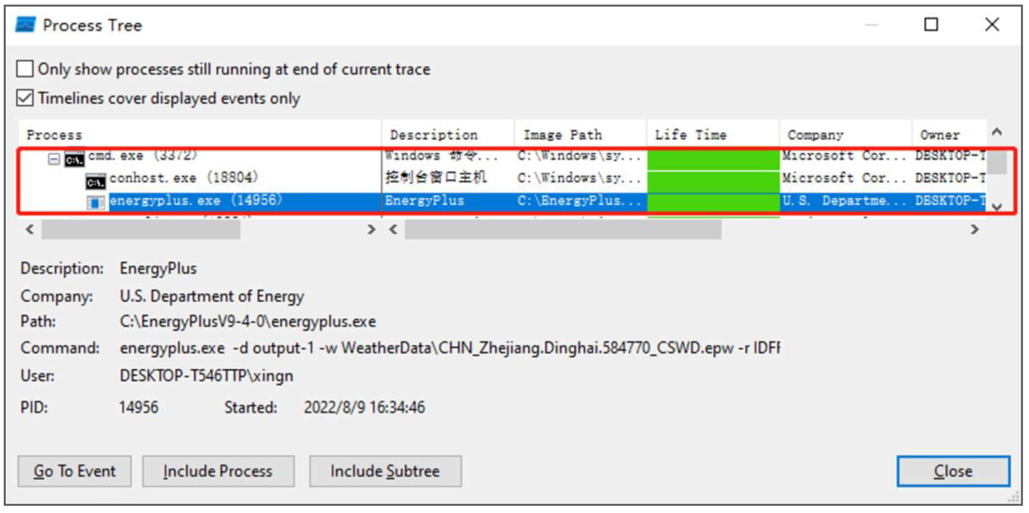
2.5. Computational-Load-Metering Method and Metrics
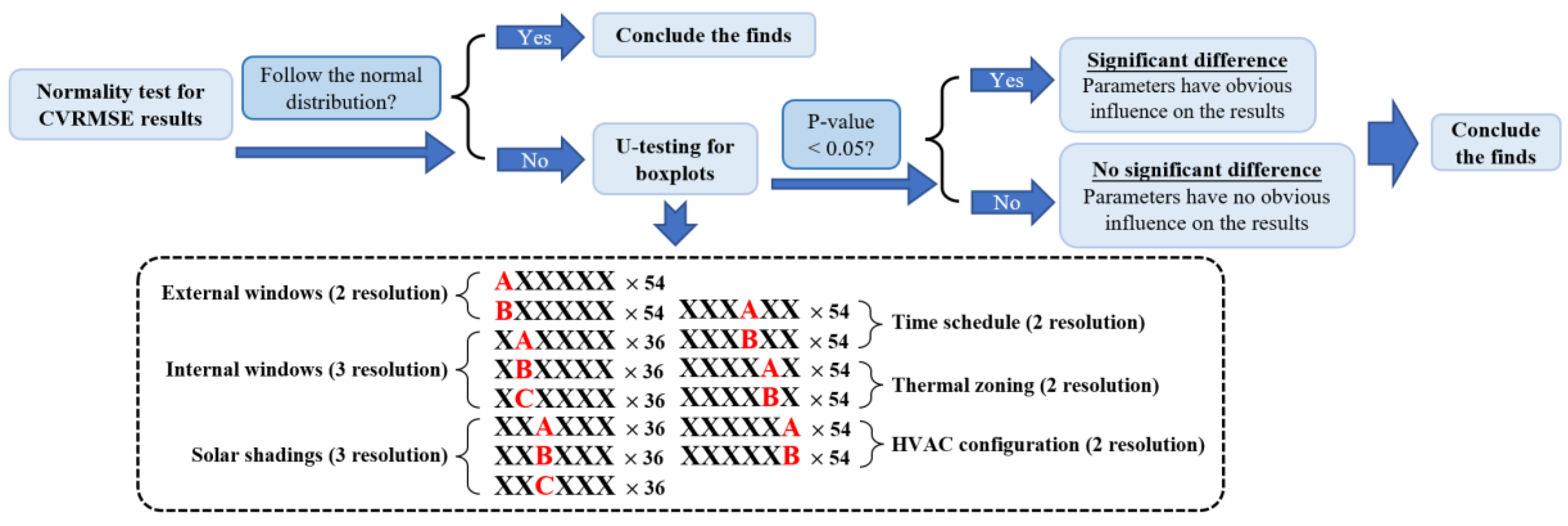
2.6. Sensitivity Analysis for Simulated Results
3. Results and Discussion
3.1. Sensitivity Analysis for Simulated Results of Model Input Parameters
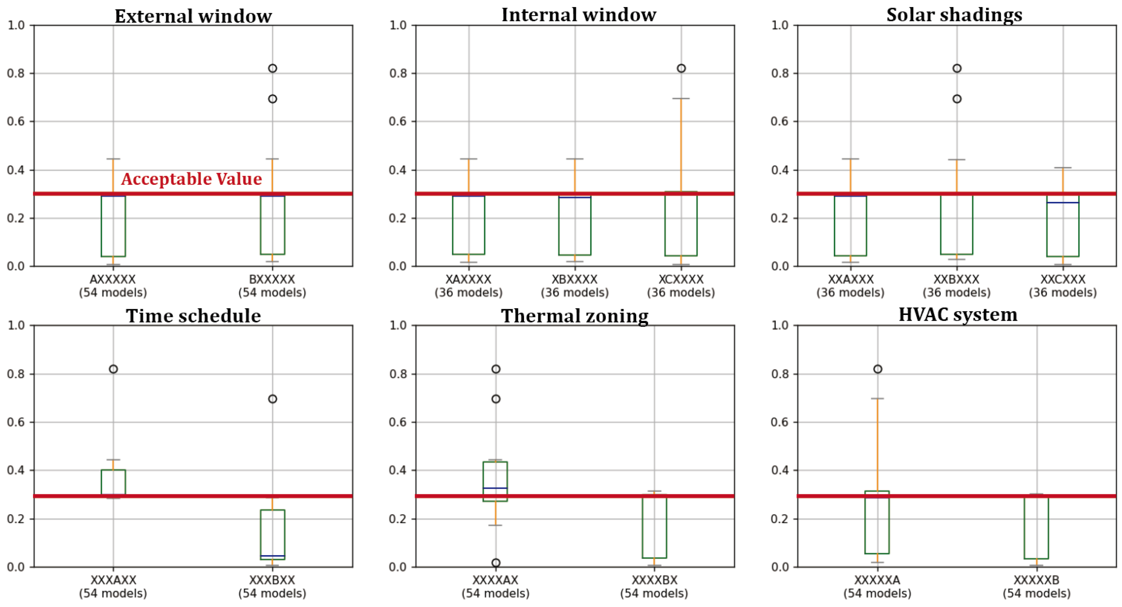
3.1.1. Sensitivity Analysis of Energy Simulation Error
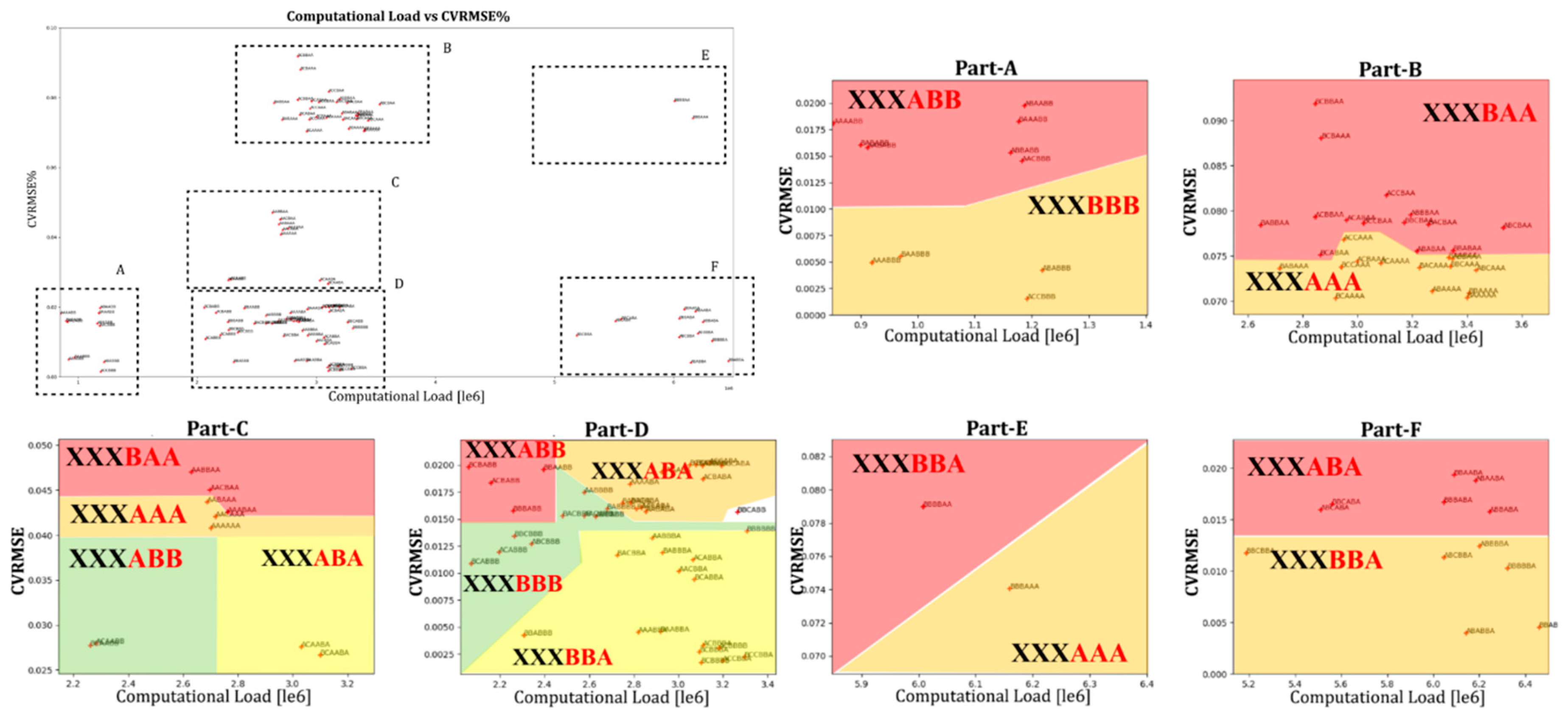
3.1.2. Sensitivity Analysis for Accuracy of Simulated Zone Mean Air Temperature
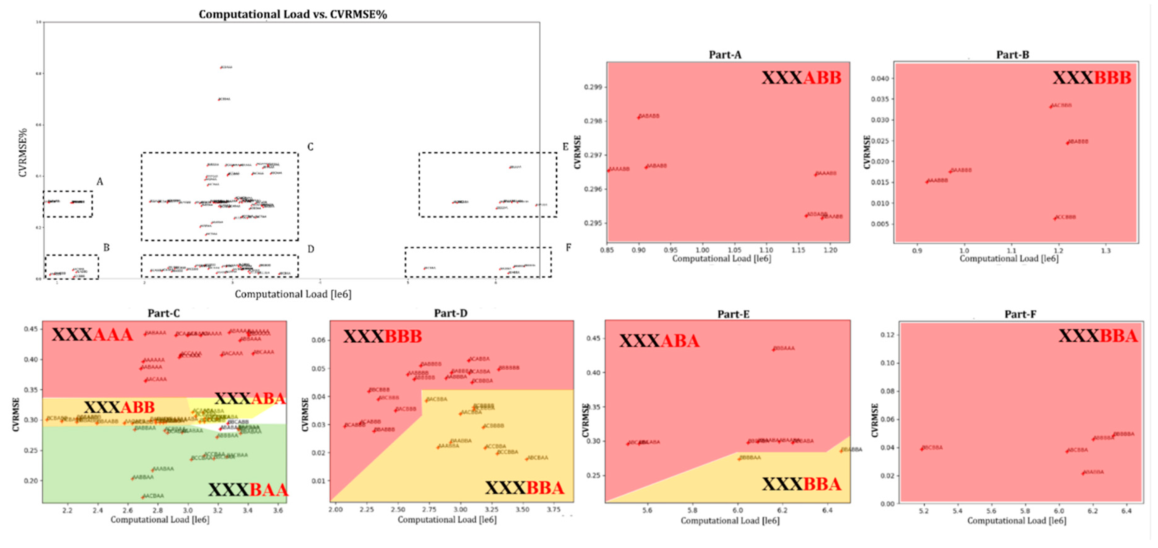
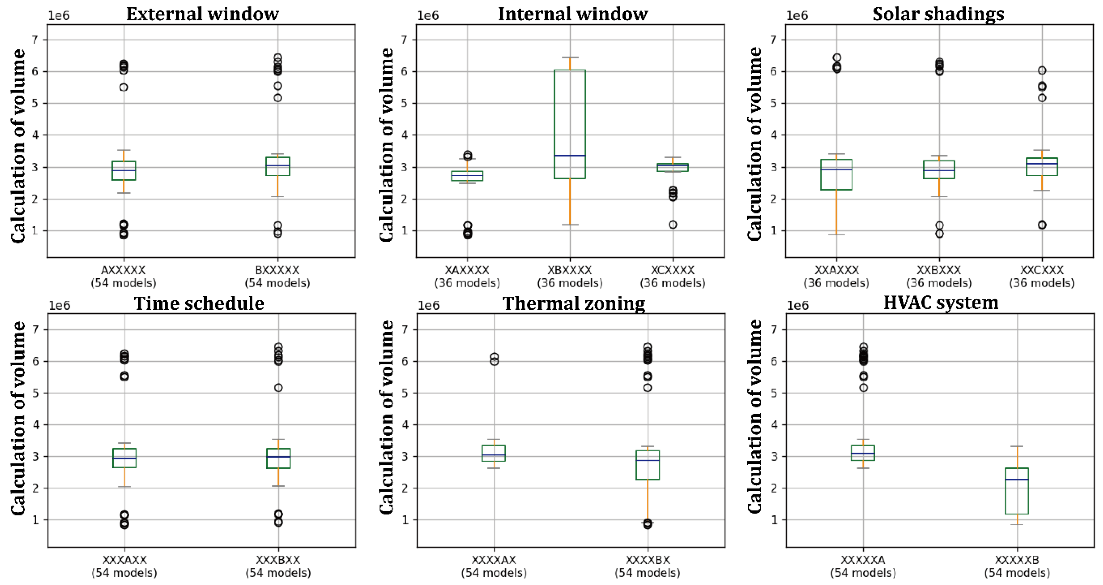
3.1.3. Sensitivity Analysis for Computational Load
3.2. Main Findings
4. Limitations and Future Work
5. Conclusions
Author Contributions
Funding
Institutional Review Board Statement
Informed Consent Statement
Data Availability Statement
Conflicts of Interest
Abbreviations
| ABM | Agent-based modelling |
| ASHRAE | The American Society of Heating, Refrigerating and Air-Conditioning Engineers |
| BEM | Building-energy modelling |
| CEA | City energy analyst |
| CityBES | City building-energy saver |
| CityGML | City geography markup language |
| CPU | Central processing unit |
| CVRMSE | Coefficient of the variation of the root mean square error |
| DB | DesignBuilder |
| EPW | EnergyPlus weather file |
| FEMP | Federal Energy Management Program |
| GPU | Graphics processing unit |
| HVAC | Heating, ventilation and air conditioning |
| IDF | (EnergyPlus) input data file |
| IPMVP | International Performance Measurement and Verification Protocol |
| LBNL | Lawrence Berkeley National Laboratory |
| LOD | Level of detail |
| MBE | Mean bias error |
| NMBE | Normalised mean bias error |
| OB | Occupant behavior |
| PID | Process identifier |
| PIS | Performance-index system |
| SA | Sensitivity analysis |
| TMY | Typical meteorological year |
| UBEM | Urban building-energy modelling |
| UMI | Urban modelling interface |
| VRF | Variable refrigerant flow |
| WWR | Window-to-wall ratio |
Appendix A

| ID | Settings | E+ CPU Computational Load | E+ Run Time | ID | Settings | E+ CPU Computational Load | E+ Run Time |
|---|---|---|---|---|---|---|---|
| 1 | AAAAAA | 872,935 | 3 min 25.37 s | 73 | BAAAAA | 1,192,089 | 5 min 3.38 s |
| 3 | AAAABA | 2,703,294 | 17 min 1.08 s | 75 | BAAABA | 3,400,657 | 23 min 13.54 s |
| 4 | AAAABB | 2,784,328 | 17 min 1.32 s | 76 | BAAABB | 2,925,088 | 17 min 53.06 s |
| 5 | AAABAA | 852,716 | 3 min 22.79 s | 77 | BAABAA | 1,177,184 | 5 min 2.82 s |
| 7 | AAABBA | 2,763,596 | 17 min 26.11 s | 79 | BAABBA | 3,333,568 | 22 min 56.83 s |
| 8 | AAABBB | 2,821,478 | 17 min 15.26 s | 80 | BAABBB | 2,921,068 | 17 min 51.47 s |
| 9 | AABAAA | 920,342 | 4 min 17.69 s | 81 | BABAAA | 970,722 | 4 min 27.47 s |
| 11 | AABABA | 2,688,152 | 18 min 7.72 s | 83 | BABABA | 2,715,675 | 18 min 14.15 s |
| 12 | AABABB | 2,854,637 | 19 min 20.83 s | 84 | BABABB | 2,748,278 | 18 min 28.40 s |
| 13 | AABBAA | 911,960 | 4 min 16.27 s | 85 | BABBAA | 900,429 | 4 min 8.59 s |
| 15 | AABBBA | 2,631,439 | 17 min 58.90 s | 87 | BABBBA | 2,647,489 | 17 min 49.79 s |
| 16 | AABBBB | 2,883,040 | 19 min 20.83 s | 88 | BABBBB | 2,929,964 | 19 min 26.92 s |
| 17 | AACAAA | 2,578,271 | 15 min 20.15 s | 89 | BACAAA | 2,681,124 | 16 min 51.36 s |
| 19 | AACABA | 2,718,937 | 22 min 13.66 s | 91 | BACABA | 3,226,298 | 28 min 19.73 s |
| 20 | AACABB | 2,834,987 | 22 min 44.08 s | 92 | BACABB | 2,786,431 | 22 min 15.11 s |
| 21 | AACBAA | 2,578,402 | 15 min 20.91 s | 93 | BACBAA | 2,813,418 | 17 min 54.77 s |
| 23 | AACBBA | 2,698,924 | 22 min 11.74 s | 95 | BACBBA | 3,259,841 | 28 min 30.02 s |
| 24 | AACBBB | 3,002,144 | 24 min 9.70 s | 96 | BACBBB | 2,726,666 | 21 min 47.44 s |
| 25 | ABAAAA | 1,182,886 | 5 min 18.65 s | 97 | BBAAAA | 2,481,732 | 12 min 3.99 s |
| 27 | ABAABA | 3,273,823 | 22 min 26.28 s | 99 | BBAABA | 3,407,245 | 23 min 31.09 s |
| 28 | ABAABB | 6,184,080 | 49 min 15.79 s | 100 | BBAABB | 6,090,232 | 48 min 20.18 s |
| 29 | ABABAA | 1,187,397 | 5 min 20.44 s | 101 | BBABAA | 2,396,211 | 11 min 40.21 s |
| 31 | ABABBA | 3,216,672 | 23 min 13.92 s | 103 | BBABBA | 3,350,001 | 23 min 2.48 s |
| 32 | ABABBB | 6,143,588 | 49 min 8.99 s | 104 | BBABBB | 6,460,217 | 50 min 58.13 s |
| 33 | ABBAAA | 1,219,083 | 6 min 2.77 s | 105 | BBBAAA | 2,307,666 | 13 min 32.13 s |
| 35 | ABBABA | 3,347,326 | 24 min 41.65 s | 107 | BBBABA | 6,160,184 | 52 min 26.27 s |
| 36 | ABBABB | 6,245,233 | 54 min 38.55 s | 108 | BBBABB | 6,047,524 | 52 min 0.17 s |
| 37 | ABBBAA | 1,162,875 | 5 min 47.94 s | 109 | BBBBAA | 2,260,476 | 13 min 16.66 s |
| 39 | ABBBBA | 3,195,144 | 23 min 33.74 s | 111 | BBBBBA | 6,007,941 | 51 min 56.35 s |
| 40 | ABBBBB | 6,202,873 | 54 min 4.62 s | 112 | BBBBBB | 6,322,800 | 54 min 24.80 s |
| 41 | ABCAAA | 2,629,003 | 16 min 27.83 s | 113 | BBCAAA | 3,307,930 | 23 min 4.25 s |
| 43 | ABCABA | 3,434,408 | 30 min 10.40 s | 115 | BBCABA | 3,340,054 | 29 min 21.96 s |
| 44 | ABCABB | 5,511,089 | 54 min 31.49 s | 116 | BBCABB | 5,561,624 | 54 min 18.75 s |
| 45 | ABCBAA | 2,629,652 | 16 min 28.86 s | 117 | BBCBAA | 3,265,198 | 22 min 53.24 s |
| 47 | ABCBBA | 3,533,039 | 31 min 15.76 s | 119 | BBCBBA | 3,172,339 | 27 min 51.24 s |
| 48 | ABCBBB | 6,047,434 | 58 min 6.95 s | 120 | BBCBBB | 5,187,088 | 53 min 47.40 s |
| 49 | ACAAAA | 2,343,145 | 10 min 14.55 s | 121 | BCAAAA | 2,265,731 | 9 min 54.78 s |
| 51 | ACAABA | 3,085,432 | 19 min 24.26 s | 123 | BCAABA | 2,920,421 | 18 min 7.37 s |
| 52 | ACAABB | 3,032,752 | 19 min 9.01 s | 124 | BCAABB | 3,100,417 | 19 min 33.95 s |
| 53 | ACABAA | 2,281,977 | 9 min 58.81 s | 125 | BCABAA | 2,261,130 | 9 min 55.28 s |
| 55 | ACABBA | 2,961,297 | 18 min 39.90 s | 127 | BCABBA | 2,864,269 | 17 min 59.32 s |
| 56 | ACABBB | 3,066,746 | 19 min 30.44 s | 128 | BCABBB | 3,072,478 | 19 min 28.13 s |
| 57 | ACBAAA | 2,197,463 | 10 min 58.16 s | 129 | BCBAAA | 2,072,501 | 10 min 12.77 s |
| 59 | ACBABA | 2,999,387 | 20 min 53.98 s | 131 | BCBABA | 2,868,314 | 19 min 36.43 s |
| 60 | ACBABB | 3,111,566 | 21 min 46.30 s | 132 | BCBABB | 3,050,689 | 21 min 5.81 s |
| 61 | ACBBAA | 2,161,255 | 10 min 48.16 s | 133 | BCBBAA | 2,061,223 | 10 min 10.28 s |
| 63 | ACBBBA | 2,847,068 | 19 min 54.61 s | 135 | BCBBBA | 2,845,895 | 19 min 26.21 s |
| 64 | ACBBBB | 3,110,233 | 21 min 56.79 s | 136 | BCBBBB | 3,095,251 | 21 min 30.95 s |
| 65 | ACCAAA | 3,181,930 | 20 min 26.24 s | 137 | BCCAAA | 3,103,430 | 19 min 57.69 s |
| 67 | ACCABA | 2,950,062 | 24 min 5.89 s | 139 | BCCABA | 2,942,245 | 24 min 2.18 s |
| 68 | ACCABB | 3,139,733 | 25 min 48.53 s | 140 | BCCABB | 3,194,726 | 26 min 18.74 s |
| 69 | ACCBAA | 3,109,277 | 19 min 54.87 s | 141 | BCCBAA | 3,078,908 | 19 min 56.84 s |
| 71 | ACCBBA | 3,105,977 | 25 min 24.61 s | 143 | BCCBBA | 3,022,444 | 24.39 min 46 s |
| 72 | ACCBBB | 3,197,998 | 26 min 41.79 s | 144 | BCCBBB | 3,296,785 | 27 min 3.48 s |
References
- Rehman, A.; Ma, H.; Ozturk, I.; Ulucak, R. Sustainable development and pollution: The effects of CO2 emission on population growth, food production, economic development, and energy consumption in Pakistan. Environ. Sci. Pollut. Res. 2021, 29, 17319–17330. [Google Scholar] [CrossRef] [PubMed]
- International Energy Agency (IEA). Global Energy Review: CO2 Emissions in 2021 Global Emissions Rebound Sharply to Highest Ever Level; International Energy Agency (IEA): Paris, France, 2021; Available online: https://iea.blob.core.windows.net/assets/c3086240-732b-4f6a-89d7-db01be018f5e/GlobalEnergyReviewCO2Emissionsin2021.pdf (accessed on 31 July 2022).
- Cao, X.; Dai, X.; Liu, J. Building energy-consumption status worldwide and the state-of-the-art technologies for zero-energy buildings during the past decade. Energy Build. 2016, 128, 198–213. [Google Scholar] [CrossRef]
- Nelson, F. A review on the basics of building energy estimation. Renew. Sustain. Energy Rev. 2014, 31, 53–60. [Google Scholar] [CrossRef]
- Ciardiello, A.; Rosso, F.; Dell’Olmo, J.; Ciancio, V.; Ferrero, M.; Salata, F. Multi-objective approach to the optimization of shape and envelope in building energy design. Appl. Energy 2020, 280, 115984. [Google Scholar] [CrossRef]
- Birdsall, B.; Buhl, W.F.; Ellington, K.L.; Erdem, A.E.; Winkelmann, F.C. Overview of the DOE-2 Building Energy Analysis Program; Report LBL-19735; Lawrence Berkeley Laboratory: Berkeley, CA, USA, 1990; Available online: https://escholarship.org/content/qt8gm226b0/qt8gm226b0.pdf (accessed on 4 August 2022).
- Crawley, D.B.; Lawrie, L.K.; Winkelmann, F.C.; Buhl, W.F.; Huang, Y.J.; Pedersen, C.O.; Strand, R.K.; Liesen, R.J.; Fisher, D.E.; Witte, M.J.; et al. EnergyPlus: Creating a new-generation building energy simulation program. Energy Build. 2001, 33, 319–331. [Google Scholar] [CrossRef]
- Yan, D.; Jiang, Y. An Overview of an Integrated Building Simulation Tool-Designer’s Simulation Toolkit (DeST). In Proceedings of the Ninth International IBPSA Conference, Montréal, QC, Canada, 15–18 August 2005; Available online: http://www.ibpsa.org/proceedings/bs2005/bs05_1393_1400.pdf (accessed on 29 July 2022).
- Robinson, D.; Haldi, F.; Leroux, P.; Perez, D.; Rasheed, A.; Wilke, U. CitySim: Comprehensive Micro-Simulation of Resource Flows for Sustainable Urban Planning. In Proceedings of the Eleventh International IBPSA Conference, Glasgow, Scotland, 27–30 July 2009; pp. 1083–1090. Available online: http://ibpsa.org/proceedings/BS2009/BS09_1083_1090.pdf (accessed on 2 August 2022).
- Reinhart, C.; Dogan, T.; Jakubiec, J.A.; Rakha, T.; Sang, A. Umi-an Urban Simulation Environment for Building Energy Use, Daylighting and Walkability. In Proceedings of the 13th Conference of International Building Performance Simulation Association, Chambery, France, 26–28 August 2013; Volume 1, pp. 476–483. Available online: https://www.academia.edu/download/34334256/p_1404_Umi.pdf (accessed on 29 July 2022).
- Hong, T.; Chen, Y.; Lee, S.H.; Piette, M.A. CityBES: A Web-Based Platform to Support City-Scale Building Energy Efficiency. Urban Comput. 2016, 14, 2016. Available online: http://www2.cs.uic.edu/~urbcomp2013/urbcomp2016/papers/CityBES.pdf (accessed on 29 July 2022).
- Fonseca, J.A.; Thomas, D.; Willmann, A.; Elesawy, A.; Schlueter, A. The City Energy Analyst Toolbox V0.1. In Expanding Boundaries: Systems Thinking for the Built Environment; Vdf Publisher: Zürich, Switzerland, 2016. [Google Scholar] [CrossRef]
- Remmen, P.; Lauster, M.; Mans, M.; Fuchs, M.; Osterhage, T.; Müller, D. TEASER: An open tool for urban energy modelling of building stocks. J. Build. Perform. Simul. 2018, 11, 84–98. [Google Scholar] [CrossRef]
- Kim, E.J.; Plessis, G.; Hubert, J.L.; Roux, J.J. Urban energy simulation: Simplification and reduction of building envelope models. Energy Build. 2014, 84, 193–202. [Google Scholar] [CrossRef]
- Tian, W. A review of sensitivity analysis methods in building energy analysis. Renew. Sustain. Energy Rev. 2013, 20, 411–419. [Google Scholar] [CrossRef]
- Eisenhower, B.; O’Neill, Z.; Fonoberov, V.A.; Mezić, I. Uncertainty and sensitivity decomposition of building energy models. J. Build. Perform. Simul. 2012, 5, 171–184. [Google Scholar] [CrossRef]
- Kathrin, M.; Heo, Y.; Choudhary, R. Sensitivity analysis methods for building energy models: Comparing computational costs and extractable information. Energy Build. 2016, 133, 433–445. [Google Scholar] [CrossRef] [Green Version]
- Shimeng, H.; Hong, T. The Application of Urban Building Energy Modelling in Urban Planning. In Rethinking Sustainability Towards a Regenerative Economy; Springer: Cham, Switzerland, 2021; pp. 45–63. Available online: https://library.oapen.org/bitstream/handle/20.500.12657/50031/1/978-3-030-71819-0.pdf (accessed on 30 July 2022).
- Troup, L.; Phillips, R.; Eckelman, M.J.; Fannon, D. Effect of window-to-wall ratio on measured energy consumption in US office buildings. Energy Build. 2019, 203, 109434. [Google Scholar] [CrossRef]
- Mamdooh, A.; Benjeddou, O. Impact of window to wall ratio on energy loads in hot regions: A study of building energy performance. Energies 2021, 14, 1080. [Google Scholar] [CrossRef]
- Gustavsen, A.; Thue, J.V.; Blom, P.; Dalehaug, A.; Aurlien, T.; Grynning, S.; Uvsløkk, S. Kuldebroer–Beregning, Kuldebroverdier og Innvirkning på Energibruk. 2008. Available online: https://www.sintef.no/globalassets/upload/byggforsk/bibliotek/sb_prosjektrapport_25.pdf (accessed on 30 July 2022).
- Misiopecki, C.; Bouquin, M.; Gustavsen, A.; Jelle, B.P. Thermal modelling and investigation of the most energy-efficient window position. Energy Build. 2018, 158, 1079–1086. [Google Scholar] [CrossRef]
- ASHRAE. ASHRAE Handbook: Fundamentals. American Society of Heating, Refrigeration and Air-Conditioning Engineers. 2009. Available online: https://shop.iccsafe.org/media/wysiwyg/material/8950P217-toc.pdf (accessed on 29 July 2022).
- Kirimtat, A.; Koyunbaba, B.K.; Chatzikonstantinou, I.; Sariyildiz, S. Review of simulation modelling for shading devices in buildings. Renew. Sustain. Energy Rev. 2016, 53, 23–49. [Google Scholar] [CrossRef]
- Yoshino, H.; Hong, T.; Nord, N. IEA EBC annex 53: Total energy use in buildings—Analysis and evaluation methods. Energy Build. 2017, 152, 124–136. [Google Scholar] [CrossRef] [Green Version]
- Yan, D.; O’Brien, W.; Hong, T.; Feng, X.; Gunay, H.B.; Tahmasebi, F.; Mahdavi, A. Occupant behavior modelling for building performance simulation: Current state and future challenges. Energy Build. 2015, 107, 264–278. [Google Scholar] [CrossRef] [Green Version]
- Heydarian, A.; McIlvennie, C.; Arpan, L.; Yousefi, S.; Syndicus, M.; Schweiker, M.; Mahdavi, A. What drives our behaviors in buildings? A review on occupant interactions with building systems from the lens of behavioral theories. Build. Environ. 2020, 179, 106928. [Google Scholar] [CrossRef]
- Happle, G.; Fonseca, J.A.; Schlueter, A. A review on occupant behavior in urban building energy models. Energy Build. 2018, 174, 276–292. [Google Scholar] [CrossRef] [Green Version]
- Arno, S.; Thesseling, F. Building information model based energy/exergy performance assessment in early design stages. Autom. Constr. 2009, 18, 153–163. [Google Scholar] [CrossRef]
- Shin, M.; Jeff, S.H. Thermal zoning for building HVAC design and energy simulation: A literature review. Energy Build. 2019, 203, 109429. [Google Scholar] [CrossRef]
- Wei, W.; Skye, H.M. Net-zero nation: HVAC and PV systems for residential net-zero energy buildings across the United States. Energy Convers. Manag. 2018, 177, 605–628. [Google Scholar] [CrossRef]
- Stadler, M.; Firestone, R.; Curtil, D.; Marnay, C. On-Site Generation Simulation with Energyplus for Commercial Buildings; No. LBNL-60204; Lawrence Berkeley National Lab. (LBNL): Berkeley, CA, USA, 2006. Available online: https://www.osti.gov/servlets/purl/883118-4C7tSU/ (accessed on 29 July 2022).
- DesignBuilder. DesignBuilder Ltd. 2020. Available online: http://www.designbuilder.co.uk (accessed on 28 July 2022).
- Ahn, K.U.; Kim, Y.J.; Park, C.S.; Kim, I.; Lee, K. BIM interface for full vs. semi-automated building energy simulation. Energy Build. 2014, 68, 671–678. [Google Scholar] [CrossRef]
- Ruben, B.; Saelens, D. Modelling uncertainty in district energy simulations by stochastic residential occupant behaviour. J. Build. Perform. Simul. 2016, 9, 431–447. [Google Scholar] [CrossRef]
- Adrian, C.; Augenbroe, G.; Yan, D. Occupancy data at different spatial resolutions: Building energy performance and model calibration. Appl. Energy 2021, 286, 116492. [Google Scholar] [CrossRef]
- Sanam, D.; Panchabikesan, K.; Eicker, U. Occupant-centric urban building energy modeling: Approaches, inputs, and data sources-A review. Energy Build. 2022, 257, 111809. [Google Scholar] [CrossRef]
- Korolija, I.; Marjanovic-Halburd, L.; Zhang, Y.; Hanby, V.I. Influence of building parameters and HVAC systems coupling on building energy performance. Energy Build. 2011, 43, 1247–1253. [Google Scholar] [CrossRef]
- Minjae, S.; Haberl, J.S. A procedure for automating thermal zoning for building energy simulation. J. Build. Eng. 2022, 46, 103780. [Google Scholar] [CrossRef]
- Xavier, F.; Johansson, T.; Pasichnyi, O. 262 Impacts of the Level of Details, Shadowing and Thermal Zoning on Urban Building Energy Modelling (UBEM) on a District Scale. 2021. Available online: https://www.researchgate.net/profile/Oleksii-Pasichnyi/publication/354473778_Impacts_of_the_level_of_details_shadowing_and_thermal_zoning_on_urban_building_energy_modelling_UBEM_on_a_district_scale/links/613a238d35e5e82234191c20/Impacts-of-the-level-of-details-shadowing-and-thermal-zoning-on-urban-building-energy-modelling-UBEM-on-a-district-scale.pdf (accessed on 7 January 2023).
- Johari, F.; Munkhammar, J.; Shadram, F.; Widén, J. Evaluation of simplified building energy models for urban-scale energy analysis of buildings. Build. Environ. 2022, 211, 108684. [Google Scholar] [CrossRef]
- Heine, K.M.; Choudhary, R.; Petersen, S. Bayesian calibration of building energy models: Comparison of predictive accuracy using metered utility data of different temporal resolution. Energy Procedia 2017, 122, 277–282. [Google Scholar] [CrossRef]
- Fazel, K.; Bollinger, A.; Heer, P. Temporal resolution of measurements and the effects on calibrating building energy models. arXiv 2020, arXiv:2011.08974. [Google Scholar] [CrossRef]
- Heine, K.M.; Petersen, S. Choosing the appropriate sensitivity analysis method for building energy model-based investigations. Energy Build. 2016, 130, 166–176. [Google Scholar] [CrossRef]
- Yang, S.; Tian, W.; Cubi, E.; Meng, Q.; Liu, Y.; Wei, L. Comparison of sensitivity analysis methods in building energy assessment. Procedia Eng. 2016, 146, 174–181. [Google Scholar] [CrossRef] [Green Version]
- Anh-Tuan, N.; Reiter, S. A performance comparison of sensitivity analysis methods for building energy models. Build. Simul. 2015, 8, 651–664. [Google Scholar] [CrossRef]
- Sanchez, D.G.; Lacarriere, B.; Musy, M.; Bourges, B. Application of sensitivity analysis in building energy simulations: Combining first-and second-order elementary effects methods. Energy Build. 2014, 68, 741–750. [Google Scholar] [CrossRef] [Green Version]
- Delgarm, N.; Sajadi, B.; Azarbad, K.; Delgarm, S. Sensitivity analysis of building energy performance: A simulation-based approach using OFAT and variance-based sensitivity analysis methods. J. Build. Eng. 2018, 15, 181–193. [Google Scholar] [CrossRef]
- Ye, Y.; Hinkelman, K.; Zhang, J.; Zuo, W.; Wang, G. A methodology to create prototypical building energy models for existing buildings: A case study on US religious worship buildings. Energy Build. 2019, 194, 351–365. [Google Scholar] [CrossRef]
- Hong, Y.; Deng, W.; Ezeh, C.I. Low-rise office retrofit: Prerequisite for sustainable and green buildings in Shanghai. In IOP Conference Series: Earth and Environmental Science; IOP Publishing: Beijing, China, 2019; Volume 281. [Google Scholar] [CrossRef]
- Hong, Y.; Ezeh, C.I.; Deng, W.; Hong, S.H.; Peng, Z.; Tang, Y. Correlation between building characteristics and associated energy consumption: Prototyping low-rise office buildings in Shanghai. Energy Build. 2020, 217, 109959. [Google Scholar] [CrossRef]
- Crawley, D.B.; Lawrie, L.K.; Winkelmann, F.C.; Pedersen, C.O. EnergyPlus: New Capabilities in a Whole-Building Energy Simulation Program. In Proceedings of the 7th International IBPSA Conference, Rio de Janeiro, Brazil, 13–15 August 2001; Springer: Berlin/Heidelberg, Germany, 2001. Available online: https://citeseerx.ist.psu.edu/document?repid=rep1&type=pdf&doi=5a10d09ad45fe3ccc5a0874a8983596fb772e0c8 (accessed on 12 August 2022).
- Rahmi, A. The role of building thermal simulation for energy efficient building design. Energy Procedia 2014, 47, 217–226. [Google Scholar] [CrossRef] [Green Version]
- Python. Why Python? Python Releases Wind. 2021. Available online: https://citeseerx.ist.psu.edu/document?repid=rep1&type=pdf&doi=1f2ee3831eebfc97bfafd514ca2abb7e2c5c86bb (accessed on 3 March 2023).
- Benjamin, K.; Najafi, H. A Novel Approach for Optimizing Building Energy Models Using Machine Learning Algorithms. Energies 2023, 16, 1033. [Google Scholar] [CrossRef]
- Yixing, C.; Luo, X.; Hong, T. An Agent-Based Occupancy Simulator for Building Performance Simulation; Lawrence Berkeley National Laboratory: Berkeley, CA, USA, 2016; Available online: https://escholarship.org/content/qt0047c6c3/qt0047c6c3.pdf (accessed on 13 August 2022).
- ANSI/ASHRAE/IES Standard 90.1-2016; Energy Standard for Buildings Except Low-Rise Residential Buildings (I-P Edition). The American Society of Heating, Refrigerating and Air-Conditioning Engineers: Peachtree Corners, GA, USA, 2016. Available online: https://webstore.ansi.org/Standards/ASHRAE/ANSIASHRAEIESStandard902016 (accessed on 2 August 2022).
- Wang, H.; Xu, P.; Sha, H.; Gu, J.; Xiao, T.; Yang, Y.; Zhang, D. BIM-based automated design for HVAC system of office buildings—An experimental study. Build. Simul. 2022, 15, 1177–1192. [Google Scholar] [CrossRef]
- Guideline, ASHRAE Measurement of energy, demand, and water savings. In ASHRAE Guideline; The American Society of Heating, Refrigerating and Air-Conditioning Engineers: Peachtree Corners, GA, USA, 2014; Volume 4, 150p, Available online: https://upgreengrade.ir/admin_panel/assets/images/books/ASHRAE%20Guideline%2014-2014.pdf (accessed on 3 August 2022).
- FEMP. M&V Guidelines: Measurement and Verification for Federal Energy Projects Version 3.0; Energy Efficiency and Renewable Energy: Washington, DC, USA, 2008; Available online: https://files.hudexchange.info/resources/documents/M-V-Guidelines-Measurement-Verification-Federal-Energy-Projects.pdf (accessed on 28 July 2022).
- John, C. International Performance Measurement and Verification Protocol: Concepts and Options for Determining Energy and Water Savings—Vol. I. In International Performance Measurement & Verification Protocol; Lawrence Berkeley National Laboratory: Berkeley, CA, USA, 2002; Volume 1, Available online: https://escholarship.org/content/qt68b7v8rd/qt68b7v8rd.pdf (accessed on 21 March 2023).
- Reddy, T.A.; Maor, I.; Jian, S.; Panjapornporn, C. Procedures for reconciling computer-calculated results with measured energy data. ASHRAE Res. Proj. 2006, 1051, 1–60. [Google Scholar]
- Coakley, D.; Raftery, P.; Keane, M. A review of methods to match building energy simulation models to measured data. Renew. Sustain. Energy Rev. 2014, 37, 123–141. [Google Scholar] [CrossRef] [Green Version]
- Ramos Ruiz, G.; Fernandez Bandera, C. Validation of calibrated energy models: Common errors. Energies 2017, 10, 1587. [Google Scholar] [CrossRef] [Green Version]
- Moriasi, D.N.; Arnold, J.G.; Van Liew, M.W.; Bingner, R.L.; Harmel, R.D.; Veith, T.L. Model evaluation guidelines for systematic quantification of accuracy in watershed simulations. Trans. ASABE 2007, 50, 885–900. [Google Scholar] [CrossRef]
- American Society of Heating, & Refrigerating and Air-Conditioning Engineers. In ASHRAE Handbook: Fundamentals; The American Society of Heating, Refrigerating and Air-Conditioning Engineers: Peachtree Corners, GA, USA, 2005; Available online: https://shop.iccsafe.org/media/wysiwyg/material/8950P203-toc.pdf (accessed on 29 July 2022).
- Thumann, A.; Woodroof, E. International Performance Measurement & Verification Protocol. In Handbook of Financing Energy Projects; CRC Press: Boca Raton, FL, USA, 2001; p. 249. Available online: https://core.ac.uk/download/pdf/186932674.pdf (accessed on 30 July 2022).
- Haberl, J.S.; Claridge, D.E.; Culp, C. ASHRAE’s Guideline 14-2002 for Measurement of Energy and Demand Savings: How to Determine What was Really Saved by the Retrofit. In Proceedings of the roceedings of the 5th International Conference for Enhanced Building Operations, Pittsburgh, PA, USA, 11–13 October 2005; Available online: https://oaktrust.library.tamu.edu/bitstream/handle/1969.1/5147/ESL-IC-05-10-50.pdf?sequence=4 (accessed on 31 July 2022).
- EVO. International Performance Measurement & Verification Protocol; Efficiency Valuation Organisation: Washington, DC, USA, 2007. [Google Scholar]
- Balkrushna, K.A. Crypto Ransomware Analysis and Detection Using Process Monitor. Master’s Thesis, The University of Texas at Arlington, Arlington, TX, USA, 2017. [Google Scholar]
- Saltelli, A.; Ratto, M.; Andres, T.; Campolongo, F.; Cariboni, J.; Gatelli, D.; Tarantola, S. Global Sensitivity Analysis: The Primer; John Wiley & Sons: Hoboken, NJ, USA, 2008. [Google Scholar] [CrossRef] [Green Version]
- Pianosi, F.; Beven, K.; Freer, J.; Hall, J.W.; Rougier, J.; Stephenson, D.B.; Wagener, T. Sensitivity analysis of environmental models: A systematic review with practical workflow. Environ. Model. Softw. 2016, 79, 214–232. [Google Scholar] [CrossRef]
- Pianosi, F.; Beven, K.; Freer, J.; Hall, J.W.; Rougier, J.; Stephenson, D.B.; Wagener, T. Factorial sampling plans for preliminary computational experiments. Technometrics 1991, 33, 161–174. [Google Scholar] [CrossRef] [Green Version]
- MacFarland, T.W.; Yates, J.M. Mann–Whitney U Test. In Introduction to Nonparametric Statistics for the Biological Sciences Using R; Springer: Cham, Switzerland, 2016; pp. 103–132. [Google Scholar]
- Lauzet, N.; Rodler, A.; Musy, M.; Azam, M.H.; Guernouti, S.; Mauree, D.; Colinart, T. How building energy models take the local climate into account in an urban context–A review. Renew. Sustain. Energy Rev. 2019, 116, 109390. [Google Scholar] [CrossRef]
- Tsoka, S.; Tolika, K.; Theodosiou, T.; Tsikaloudaki, K.; Bikas, D. A method to account for the urban microclimate on the creation of ‘typical weather year’datasets for building energy simulation, using stochastically generated data. Energy Build. 2018, 165, 270–283. [Google Scholar] [CrossRef]
- Ma, R.; Wang, T.; Wang, Y.; Chen, J. Tuning urban microclimate: A morpho-patch approach for multi-scale building group energy simulation. Sustain. Cities Soc. 2022, 76, 103516. [Google Scholar] [CrossRef]
- Natanian, J.; Maiullari, D.; Yezioro, A.; Auer, T. Synergetic urban microclimate and energy simulation parametric workflow. J. Phys. Conf. Ser. 2019, 1343, 012006. [Google Scholar] [CrossRef]
- Davis, J.A., III; Nutter, D.W. Occupancy diversity factors for common university building types. Energy Build. 2010, 42, 1543–1551. [Google Scholar] [CrossRef]
- Simona, D.; Hong, T. Occupancy schedules learning process through a data mining framework. Energy Build. 2015, 88, 395–408. [Google Scholar] [CrossRef] [Green Version]
- Andersen, P.D.; Iversen, A.; Madsen, H.; Rode, C. Dynamic modelling of presence of occupants using inhomogeneous Markov chains. Energy Build. 2014, 69, 213–223. [Google Scholar] [CrossRef]
- Davide, C.; Wesseling, M.T.; Müller, D. WinProGen: A Markov-Chain-based stochastic window status profile generator for the simulation of realistic energy performance in buildings. Build. Environ. 2018, 136, 240–258. [Google Scholar] [CrossRef]
- João, V.; Neves-Silva, R. Stochastic models for building energy prediction based on occupant behavior assessment. Energy Build. 2012, 53, 183–193. [Google Scholar] [CrossRef]
- Diao, L.; Sun, Y.; Chen, Z.; Chen, J. Modelling energy consumption in residential buildings: A bottom-up analysis based on occupant behavior pattern clustering and stochastic simulation. Energy Build. 2017, 147, 47–66. [Google Scholar] [CrossRef]
- Lee, Y.S.; Malkawi, A.M. Simulating multiple occupant behaviors in buildings: An agent-based modelling approach. Energy 2014, 69, 407–416. [Google Scholar] [CrossRef]
- Jared, L.; Wen, J.; Gurian, P.L. Simulating the human-building interaction: Development and validation of an agent-based model of office occupant behaviors. Build. Environ. 2015, 88, 27–45. [Google Scholar] [CrossRef]
- Jia, M.; Srinivasan, R.S.; Ries, R.; Weyer, N.; Bharathy, G. A systematic development and validation approach to a novel agent-based modeling of occupant behaviors in commercial buildings. Energy Build. 2019, 199, 352–367. [Google Scholar] [CrossRef]
- Bing, D.; Lam, K.P. Building energy and comfort management through occupant behaviour pattern detection based on a large-scale environmental sensor network. J. Build. Perform. Simul. 2011, 4, 359–369. [Google Scholar] [CrossRef]


| Facade and Orientation | Front Elevation Southern Face |
| Floor Shape | Rectangular |
| Floor Dimensions | 64.7 m × 70.1 m |
| Total Height | 17.2 m |
| Window-to-Wall Ratio | 0.35 (east), 0.4 (south), 0.33 (west), 0.34 (north) |
| Thermal-Performance U-Value (W/m2K) | 0.67 (roof), 1.0 (wall), 3.4 (windows) |
| Total Energy-Transmittance Coefficient of Windows G-value | 0.691 |
| Item | Resolution Description | Annotation No. | Image | ||
|---|---|---|---|---|---|
| Openings | External Windows (Two Levels) | / | Photo | / | 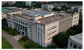 |
| A | A WWR value entered for the entire building (0.355) | ① | 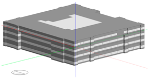 | ||
| B | Layout based on the actual situation | / | 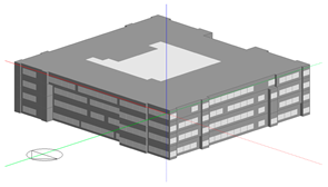 | ||
| Internal Windows (Three Levels) | / | Photo | / | 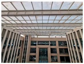 | |
| A | No internal windows | / |  | ||
| B | Utilises DB’s internal glazing templates. | ② |  | ||
| C | Layout based on the actual situation | / | 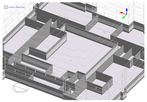 | ||
| Solar Shading (Three Levels) | / | Photos | / |  | |
| A | No solar shading | / |  | ||
| B | Utilises DB’s default overhang shadings | ③ |  | ||
| C | Layout based on the actual situation | / |  | ||
| Occupancy Schedule (Two Levels) | A | Default typical activity template provided with DB | ④ |  | |
| B | Uses high-resolution occupancy profile | ⑤ | 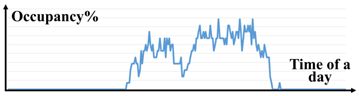 | ||
| Thermal Zoning (Two Levels) | A | Divides the building into internal and external zones based on 6.86 m depth | ⑥ | 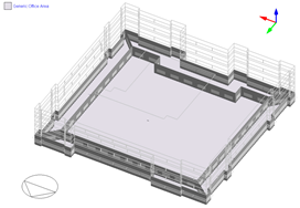 | |
| B | Based on the real layout; the rooms are merged with the same orientation and type | ⑦ | 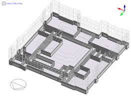 | ||
| HVAC System (Two Levels) | A | Default autosized VRF AC model provided with DB | / | 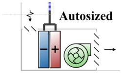 | |
| B | Custom VRF AC: heating/cooling capacity and airflow rate for VRF AC system set based on actual layout and configuration | ⑧ | 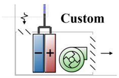 | ||
| Annotation No. | Remarks |
|---|---|
| ① | The WWR value of the four facades of the SEB was calculated to be 0.355 based on the existing conditions. |
| ② | Utilised the 20% internal glazing template provided with the DB software. |
| ③ | Utilised the 1.0 m overhang shade provided with the DB software. |
| ④ | Utilised the standard office-building activity file provided with the DB software. |
| ⑤ | Utilised the high-resolution occupancy simulator developed by Chen et al. [56] |
| ⑥ | Standard thermal zoning strategies specified in Appendix G of ASHRAE Standard 90.1-2016 [57]. Specifically, Appendix G states that due to the strong interaction of building-perimeter spaces with the outdoors as a result of solar penetration, the floor height is defined as being within 15 feet (4.6 m) of windows for a typical office ceiling height of 9 to 10 feet (2.7 m to 3 m). The floor height of the building in this case (about 4.5 m) exceeded the ASHRAE standard. The computation indicated that the critical depth was 22.5 feet (6.86 m). |
| ⑦ | Based on hourly load calculations and building geometry, the HVAC system combined areas/rooms of the building into thermal zones. Specifically, two zones/rooms were considered to be merged into the same hot zone of the HVAC system if their hourly load calculations showed sufficient approximations in the time series [58]. |
| ⑧ | Customised the parameters of the VRF system using HVAC layout drawings from the engineering construction office. |
| Calibration Step | Index | Acceptable Values for ASHRAE | Acceptable Values for FRMP | Acceptable Values for IPMVP |
|---|---|---|---|---|
| Hourly | NMBE | ±10% | ±10% | ±5% |
| CVRMSE | 30% | 30% | 20% |
| BEM Input Parameter | Resolution | Statistic | p-Value | Description |
|---|---|---|---|---|
| External Windows | AXXXXX to BXXXXX | 1348.0 | 0.501 | No significant difference found |
| Internal Windows | XAXXXX to XBXXXX | 659.5 | 0.901 | No significant difference found |
| XAXXXX to XCXXXX | 568.0 | 0.371 | No significant difference found | |
| XBXXXX to XCXXXX | 568.0 | 0.371 | No significant difference found | |
| Solar Shading | XXAXXX to XXBXXX | 614.0 | 0.706 | No significant difference found |
| XXAXXX to XXCXXX | 736.0 | 0.324 | No significant difference found | |
| XXBXXX to XXCXXX | 814.5 | 0.061 | No difference found | |
| Occupancy Schedule | XXXAXX to XXXBXX | 2859.5 | Significant difference: the accuracy of the XXXAXX type was considered to be lower than that of the XXXBXX type | |
| Thermal Zoning | XXXXAX to XXXXBX | 1894.0 | Significant difference: the accuracy of the XXXXAX type was considered to be lower than that of the XXXXBX type | |
| HVAC System | XXXXXA to XXXXXB | 1665.0 | 0.011 | Significant difference: the accuracy of the XXXXXA type was considered to be lower than that of the XXXXXB type |
| BEM Input Parameter | Resolution | Statistic | p-Value | Description |
|---|---|---|---|---|
| External Windows | AXXXXX to BXXXXX | 1395.0 | 0.701 | No significant difference found |
| Internal Windows | XAXXXX to XBXXXX | 637.0 | 0.906 | No significant difference found |
| XAXXXX to XCXXXX | 576.0 | 0.421 | No significant difference found | |
| XBXXXX to XCXXXX | 613.0 | 0.680 | No significant difference found | |
| Solar Shading | XXAXXX to XXBXXX | 650.0 | 0.987 | No significant difference found |
| XXAXXX to XXCXXX | 648.0 | 1.000 | No significant difference found | |
| XXBXXX to XXCXXX | 686.0 | 0.673 | No significant difference found | |
| Occupancy Schedule | XXXAXX to XXXBXX | 1980.0 | 0.001 | Significant difference: the accuracy of the XXXAXX type was considered to be lower than that of the XXXBXX type |
| Thermal Zoning | XXXXAX to XXXXBX | 2592.0 | Significant difference: the accuracy of the XXXXAX type was considered to be lower than that of the XXXXBX type | |
| HVAC System | XXXXXA to XXXXXB | 1853.0 | 0.0001 | Significant difference: the accuracy of the XXXXXA type was considered to be lower than that of the XXXXXB type |
| BEM Input Parameter | Resolution | Statistic | p-Value | Description |
|---|---|---|---|---|
| External Windows | AXXXXX to BXXXXX | 1247.0 | 0.196 | No significant difference found |
| Internal Windows | XAXXXX to XBXXXX | 307.0 | 0.0001 | Significant difference: the computational load of the XAXXXX type was considered to be lower than that of the XBXXXX type |
| XAXXXX to XCXXXX | 345.0 | 0.0007 | Significant difference: the computational load of the XAXXXX type was considered to be lower than that of the XCXXXX type | |
| XBXXXX to XCXXXX | 969.0 | 0.0003 | Significant difference: the computational load of the XAXXXX type was considered to be higher than that of the XCXXXX type | |
| Solar Shading | XXAXXX to XXBXXX | 612.0 | 0.689 | No significant difference found |
| XXAXXX to XXCXXX | 527.0 | 0.174 | No significant difference found | |
| XXBXXX to XXCXXX | 568.0 | 0.371 | No significant difference found | |
| Occupancy Schedule | XXXAXX to XXXBXX | 1403.0 | 0.738 | No significant difference found |
| Thermal Zoning | XXXXAX to XXXXBX | 1642.0 | 0.054 | No difference found |
| HVAC System | XXXXXA to XXXXXB | 2291.0 | Significant difference: the computational load of the XXXXXA type was considered to be lower than that of the XXXXXB type |
| Input Parameters for the Building | Sensitivity-Analysis Results | |
|---|---|---|
| For Simulated Energy and Temperature | For Computational Load | |
| External Windows | U-testing results indicated that there was no statistically significant difference between the two datasets. According to the hourly CVRMSE analysis, the exterior windows’ resolution had a minor effect on the ultimate energy consumption. | Boosting the resolution of the external windows raised the computational load marginally. The U-testing, on the other hand, revealed no statistically significant difference between the two sets of data. |
| Internal Windows | Based on the hourly CVRMSE study, the modelling resolution, as with the exterior windows, had a minor effect on the annular electrical consumption. However, when the model with the highest resolution was used, the CVRMSE became unstable, which might have been the result of the complex internal windows interacting with the other input parameters. In addition, the U-test demonstrated that there was no statistically significant distinction between the three datasets. This phenomenon proved that the internal windows were not a substantial contributor to the building’s energy use. | In addition, the U-testing demonstrated that there was a statistically significant difference between the three datasets. Consequently, the resolution of the internal windows displayed an intriguing phenomenon. The intermediate resolution (XBXXXX), the default option for the internal windows, resulted in a noticeable increase in computational load. In addition, U-testing demonstrated that this dataset was, statistically, significantly larger than the other two datasets. This issue could have been the result of the default configuration increasing the number of windows, which could have increased the interaction of heat flow between adjacent zones. In addition, the high resolution (XCXXXX), based on the real scenario, increased the computational load by a small amount. |
| Solar Shading | Generally identical to the exterior windows. However, the model with the maximum resolution marginally improved the result’s stability. | The U-testing results indicated that there was no statistically significant difference between the three datasets. However, the computing load increased slightly as the model complexity grew. Typically, the computing amount of the low resolution (XXAXXX) decreased significantly in the absence of shading, indicating that the model without shading could reduce interaction between solar lighting and the internal zone to reduce the computational load. |
| Occupancy Schedule | In contrast to the previous component, the U-testing demonstrated a statistically significant difference between the two sets of data. According to the hourly CVRMSE analysis, the higher the accuracy of the occupancy schedule, the higher the pertinence to the annual electricity consumption. | The U-testing results indicated that there was no statistically significant difference between the two datasets. Therefore, it is difficult to discern the difference in computational load between the low-occupancy and high-occupancy schedules. Surprisingly, the computational load was slightly lower at the B-level input resolution than at the A-level. This could have been due to the increased speed of reading the CSV file directly from the computer’s local directory compared to that of retrieving the information from an IDF file. |
| Thermal Zoning | Similarly to the occupancy schedule, better resolution of the thermal zoning revealed an obvious impact on annual electrical consumption. | The U-testing revealed that there was no statistically significant difference between the two sets of data. More sophisticated thermal-zoning approaches had much higher computational loads in general, but this trend appeared to decrease when other input factors were equally complex. |
| HVAC System | In general, the U-testing found a statistically significant difference between the two datasets. Consequently, the effect of HVAC system resolution on energy consumption was undetectable. However, lower resolution is more volatile than higher resolution. | The U-testing indicated that the difference between the two datasets was statistically significant. Consequently, the computational quantity of the high-resolution (XXXXXB) custom HVAC value was much less than that of the low-resolution value (XXXXXA). The autosized setting could have used unique mathematical methods to determine these parameters, but the custom-value setting entered these parameters directly, resulting in less work. |
Disclaimer/Publisher’s Note: The statements, opinions and data contained in all publications are solely those of the individual author(s) and contributor(s) and not of MDPI and/or the editor(s). MDPI and/or the editor(s) disclaim responsibility for any injury to people or property resulting from any ideas, methods, instructions or products referred to in the content. |
© 2023 by the authors. Licensee MDPI, Basel, Switzerland. This article is an open access article distributed under the terms and conditions of the Creative Commons Attribution (CC BY) license (https://creativecommons.org/licenses/by/4.0/).
Share and Cite
Kong, D.; Yang, Y.; Sa, X.; Wei, X.; Zheng, H.; Shi, J.; Wu, H.; Zhang, Z. Evaluation of the Impact of Input-Data Resolution on Building-Energy Simulation Accuracy and Computational Load—A Case Study of a Low-Rise Office Building. Buildings 2023, 13, 861. https://doi.org/10.3390/buildings13040861
Kong D, Yang Y, Sa X, Wei X, Zheng H, Shi J, Wu H, Zhang Z. Evaluation of the Impact of Input-Data Resolution on Building-Energy Simulation Accuracy and Computational Load—A Case Study of a Low-Rise Office Building. Buildings. 2023; 13(4):861. https://doi.org/10.3390/buildings13040861
Chicago/Turabian StyleKong, Dezhou, Yimin Yang, Xingning Sa, Xuanyue Wei, Huoyu Zheng, Jiwei Shi, Hongyi Wu, and Zhiang Zhang. 2023. "Evaluation of the Impact of Input-Data Resolution on Building-Energy Simulation Accuracy and Computational Load—A Case Study of a Low-Rise Office Building" Buildings 13, no. 4: 861. https://doi.org/10.3390/buildings13040861