Article

Classification of Low-Strain Foundation Pile Testing Signal Using Recurrent Neural Network

1
Building Engineering Test Center, China Academy of Building Research Co., Ltd., Beijing 100013, China
2
CABR Testing Center Co., Ltd., Beijing 100013, China
*
Author to whom correspondence should be addressed.
Buildings 2023, 13(5), 1228; https://doi.org/10.3390/buildings13051228
Submission received: 27 March 2023 / Revised: 30 April 2023 / Accepted: 5 May 2023 / Published: 7 May 2023
(This article belongs to the Special Issue AI and Data Analytics for Energy-Efficient and Healthy Buildings)

Abstract

:
The testing of the foundation pile is an important means to ensure the quality of the foundation pile in the construction process, and the low-strain pile test is one of the most commonly used testing technologies. However, in order to ensure that the testing signal is effective and reliable, it is necessary to provide the preliminary judgment results when acquiring the testing signal in the field. In this paper, we propose a data classification method for low-strain pile testing data using a recurrent neural network as the core. In this method, after identification, tailoring, and normalization, the input feature vector with a sequential structure is sent into this model. The model ensures the efficient use of data values while considering the sequential relationship among the data. At last, we designed and produced one complete model pile and six asymmetric model piles, which can form thirteen kinds of testing signals. The optimal application model was selected by the 10-fold cross verification method, and the influence of increasing the input feature dimension on the accuracy was discussed. Finally, compared with the other two methods, this model has the highest accuracy, at 98.46%, but it requires more training parameters and a longer training time.

1. Introduction

In engineering construction, foundation pile has been more and more widely used in recent years, as it has good load transfer performance, adaptability to complex geological conditions, and high bearing capacity [1,2,3]. However, it is followed by the increase in pile quality problems in the construction process, so the quality test of the pile foundation is of great significance for finding problems and taking necessary remedial means to ensure the construction quality of foundation pile in a timely manner [4,5,6].
The pile quality test includes a pile integrity test and a bearing capacity test. Pile integrity is a comprehensive qualitative index that reflects the relative change of pile section size, pile material compactness, and continuity. The bearing capacity test is used to test the ultimate bearing capacity of a single pile through the experimental method and determine whether the vertical bearing capacity of the engineering pile meets the design requirements. Different testing targets need to be completed with different testing techniques. These techniques usually include: static load, core sampling drilling, dynamic testing, and the ultrasonic method. However, the static load method belongs to destructive testing and has long testing cycle and expensive cost, which is not convenient for large-scale use [7]. Core sampling drilling is only suitable for the end bearing piles with the large diameter (>lm) and relatively short pile length [8]. The ultrasonic method has the advantages of fast test speed, as well as accurate and reliable results; however, the ultrasonic method requires the embedded steel pipes in advance, which have a higher cost, more troublesome construction process, and cannot do random sampling, so it cannot be widely used [9]. In the test of pile integrity, the low-strain pile test (LSPT), which is a kind of dynamic testing method, has the characteristics of simple equipment, simple steps and low cost, so it has become a powerful means of surveying pile quality [10,11]. The industry standard of the People’s Republic of China “Technical Specification for Testing of Building Foundation Piles JGJ 106-2014” also specifies the use field and the data analysis of the LSPT. The LSPT method is suitable for testing the integrity of concrete piles and determining the degree and the location of pile defects. The characteristics of LSPT make it suitable for a wide range of surveys for foundation pile quality. In the testing technical specification, the number of foundation piles for pile integrity testing is stipulated: (1) If the design grade of the building pile foundation is Grade A, the number of tested piles shall not be less than 30% of the total number and shall not be less than 20; (2) for other pile foundation projects, the tested number should not be less than 20% of the total number of piles and should not be less than 10 piles. Therefore, there are a many foundation piles that need to be tested during construction, and LSPT is the best technical means to solve this problem.
The whole LSPT process includes two steps: field data acquisition and post-processing data analysis. Engineers use the dynamic measurement instrument (DMI) to obtain the test data of the pile and, then, evaluate the integrity of the pile through the analysis of the test data. However, the LSPT is subject to many interference factors, such as the installation position of the sensor, the bonding method, the hardness of the hammerhead, and the strength of the drop hammer. Moreover, the field technicians also need to make a preliminary judgment on the collected data, according to the specifications and the engineering information, to decide whether the data can be used or if they need to be collected repeatedly. In addition, the foundation pile test is often carried out outdoors in relatively poor conditions, and it is hoped that the outdoor process can be completed as soon as possible. This requires that the field testing equipment can automatically judge the testing data and assist the field engineer with some suggestive conclusions while collecting data. Therefore, it is necessary to rely on the basic data of in-situ pile testing and a set of artificial intelligence methods, to identify and classify these signals in time, to determine the integrity of pile body.
Artificial Intelligence (AI) has the demonstrated superior predictive ability, compared to the traditional methods, in modeling the complex behavior. This ability has made AI a popular and particularly amenable option in geotechnical engineering applications [12]. With the rapid development of computer technology and AI, some studies have attempted to establish finite element methods and neural networks (NN) for automating data analysis [13]. The finite element method mainly uses the wavelet analysis to discriminate the defect of the foundation pile [14,15]. Its outstanding advantage is that it is suitable for dealing with nonlinear, heterogeneous, and complex boundary problems. However, the finite element method needs to determine the geotechnical materials model and its parameters in advance. Due to the inherent complexity of geotechnical materials, there are many factors affecting the stress–strain relationship of the geotechnical materials, and it is unlikely to have a universally applicable model. After the geotechnical model is confirmed, the setting of the model parameters is still a big problem. A neural network is a new, self-adaptive nonlinear system developed by imitating biological systems. It can extract effective knowledge and rules from a large number of existing knowledge samples, and it can constantly adapt to environmental changes in the learning process. It is suitable for multi-parameter, nonlinear system discrimination classification, pattern recognition, evaluation prediction, etc. [16]. It especially does not need a certain model in advance. The implementation of a neural network only needs to be given a general model structure and some training samples (including input and output data), from which the relationship network between the input data and the output data is determined [17], and then, the model parameters are trained. Once trained and validated, new input data can be analyzed by the model deployed in an application [18]. In the field of the foundation pile test, many studies have applied neural networks to specific testing data analysis. Jebur et al. [19] used a new artificial neural network (ANN) method to examine pile bearing capacity and to provide a reliable model to simulate pile load–settlement behavior. Alzo’ubi et al. [20] proposed an artificial neural network approach to build a model that can predict a complete static load pile test. In this paper, it was shown that, by incorporating the pile configuration, soil properties, and groundwater table in an artificial neural network model, the static load test can be predicted with confidence. Wei W. et al. [21] proposed a prediction model of bearing capacity of the composite foundation, based on a RBF neural network, compared with the same model based on BP neural network. The prediction results of two models show that the method of predicting the bearing capacity of the composite foundation of the vibrating gravel pile, based on a RBF neural network, is more accurate than that based on a BP neural network, and it takes less time to compute. KAL Goudjil [22] proposed an artificial neural network to predict the pile deflection, compared with a numerical modeling of an experimental model, using the three-dimensional finite element method. The results obtained are very satisfactory with very acceptable errors. In the above research, neural networks have been applied to a number of foundation pile testing projects. Through the analysis and comparison, it is found that the application of neural networks in these fields has resulted in a satisfactory effect. These neural network models can then be deployed to the cloud platform, where the field testing devices can remotely connect to the cloud platform to obtain AI services [23]. In a considerable number of provinces in China, the digital construction of testing requires that the foundation pile testing data be uploaded to the monitoring platform in real time. However, at present, these platforms only record and store data, and they are unable to find the problematic data and the site pile problems reflected in the data in time. In the future, the artificial intelligence model may become a functional module in the digital platform for the real-time diagnosis of foundation pile status at the construction site.
However, the neural network approach is a general technique. In recent years, in addition to the traditional BP neural network, a variety of network models for different application scenarios, such as Convolutional Neural Network (CNN) and Recurrent Neural Network (RNN), have been expanded. CNN has the main characteristics of sparse connection and weight sharing, which are mainly applied to image processing, pattern recognition, and other fields [24]. The RNN model is suitable for the application scenarios where there is a sequential relation between input features [25]. The LSPT signal is an ordered data set that reflects the integrity of the pile obtained by the testing personnel at the testing site of the foundation pile. There is a chronological order among the points in this data set. Moreover, since the data are obtained by the physical analog through A/D sampling, each data point should change continuously. In a traditional BP neural network, there is no logical or temporal sequence between the input features, and the order changes in the ordering of features will not affect the output of the model. However, the sequential relationship among the data points is lost. Therefore, in this paper, we propose to use a combination of the RNN model and multi-layer neural network model (MLNN) to classify LSPT signals under the condition of retaining the sequential information and making full use of the advantages of neural networks.
The LSPT signal in the field is the quantitative result of a series of internal and environmental factors, which are not only related to the pile body quality but also related to the pile length, the pile body materials, and the soil around the pile. The quality of the signal acquisition can be directly affected by the hammer material, the adhesive, and the technical level of the testing technician, e.g., the force and the angle of the hammer hit on the pile top. At the current research stage, in order to reduce the complexity of the neural network model and reduce the coupling relationship among input features, we designed and processed seven model piles for the experiments. In the testing process, the influence of pile length, pile material, pile stress wave velocity, and other factors is not considered, and the relationship between the time sequence signal and the pile classification is only analyzed.
In this paper, an artificial intelligence method, based on Recurrent Neural Network (RNN) and Multi-Layer Neural Network (MLNN), is proposed to classify the foundation pile according to the LSPT testing data, which can further improve the on-site efficiency of the LSPT test. Taking full account of the characteristics of a low-strain foundation pile test, a sequential feature model based on RNN is established, and then, the complex internal neurons are connected by a multi-layer neural network so as to realize the classification of sequential signals.
The remainder of our paper is organized as follows. In Section 2, we provide the related research about the principles of LSPT and some artificial intelligence methods for pile testing data analysis. In Section 3, we propose an analysis model based on RNN and MLNN. Section 4 provides the experimental results and discussion, while the conclusions are given in Section 5.

2. Related Research

2.1. Theory of Low-Strain Pile Test (LSPT)

The LSPT mainly adopts low-energy transient vibration to make the pile particle vibrate in a low amplitude within the elastic range. The vibration reflection signal is received by the velocity sensor or the acceleration sensor, and the integrity of the pile is judged by combining the signal and the elastic wave theory [26,27,28]. Figure 1 shows the schematic diagram of the low-strain dynamic test site. The acceleration sensor is installed vertically on the pile top at position 1, as shown in Figure 1, which is about 2/3 radius away from the pile top center. While hitting position 2 with a hand hammer to generate an excitation signal, the vibration signal caused by the incident wave and the reflected wave on the pile top can be collected by the sensor on the pile top and stored by the pile dynamic measurement instrument. In the “Technical Specification for Testing of Building Foundation Piles JGJ 106-2014”, four classifications of pile integrity are specified: type 1 pile, which has a complete pile body; type 2 pile, which has some slight pile defects that do not affect the normal bearing capacity of the pile structure; type 3 pile, which has some obvious pile defects that affect the bearing capacity of the pile structure; type 4 pile, which has serious defects in the pile body. By analyzing the vibration signal, an engineer can determine whether there are defects in the tested pile and classify the pile into one of four categories.
As shown in Figure 1, the body of the foundation pile is divided into several segments along the direction of the pile body. After the pile top is hit instantly, each adjacent segment in the pile body will move along the direction of the pile body, that is, the downward propagating stress wave (incident wave) will occur. The pile is assumed to be a one-dimensional linear elastic rod model which is regarded as a homogeneous and isotropic elastic rod with an equal cross section [29,30]. Under the premise that the lateral inertia effect and the soil resistance change are ignored, Hooke’s law is satisfied, the wavelength wl is less than the pile length L, and the wavelength wl is greater than the pile diameter D, the one-dimensional rod wave equation can be established as shown in Formula (1).
2 μ t 2 c 2 2 μ x 2 = 0
where μ is the position of the pile particle, t is the propagation time of the stress wave in the pile, and c is the velocity of the stress wave propagating vertically along the rod.
If the impedance of a certain section in the pile changes, the stress wave will form the reflection and the transmission on the interface of impedance change, that is, the particle velocity v of the adjacent section at the corresponding position is affected [31,32]. According to the impedance transformation, the relationship between pile body impedance Z, elastic modulus E, pile (rod) section area A, and pile concrete density ρ is shown in Equation (2).
Z = E A / c = ρ A c
These model piles are made by unified pouring, so the density of the pile concrete ρ and the velocity of the stress wave, propagating vertically along the rod c, are basically unchanged. Therefore, when the velocity of the pile particle v changes, the change of the section area of the pile occurs, that is, the cracks and the fractures caused by the construction of the foundation pile affect the integrity of the pile. Therefore, the measured particle velocity v indirectly reflects the change of pile impedance Z. Under the condition that the tested object is the model pile, the change of pile section area affects the integrity of the pile [33,34,35,36].

2.2. Artificial Intelligence Methods for Pile Test

After obtaining the test data of the foundation pile on site, it is necessary for technical personnel to analyze the data, combined with some field information and their own experience, and classify the pile. The defect identification of the foundation pile is a highly nonlinear problem, which is difficult to express with an exact explicit function [37]. Some assumptions are made in the existing analytical formulas to reduce the complexity of the problem, but the analytical results are often much different from the actual results. At this stage, it mainly relies on the theoretical analysis and the experience of technical personnel. With the continuous development of neural network technology, the data classification technology, based on a neural network, has more realistic and research significance.
Wang et al. [38] proposed a BP Neural Network (BPN) model for identifying the integrity of the foundation pile based on the stress wave reflection wave method. The input vector in this method was composed of the testing data, which was divided into 64 segments, the pile length, the pile diameter, and the wave velocity. The output data was evenly divided into 32 unit segments along the length of the pile, and the position of each segment was a position relative to the actual pile body. The output elements of each unit segment were three, respectively, representing reduction and expansion, segregation, and fracture. This method was used to study and predict the reflected wave data of 102 immersed pipe cast-in piles in soft soil area of Tianjin. The 102 piles were divided into 2 groups. The first group of about 89 piles was used for learning, including the normal piles and the various defective piles. Another group of 13 piles, also including the normal piles and the various defective piles, was used for testing. The experimental results showed that the overall prediction accuracy can be above 90%.
Liu et al. [39] proposed the method of feature extraction by symlet wavelets and the identification of foundation pile defects by a BP neural network. In this method, the symlet wavelet was used to decompose the velocity–response curve of the foundation pile particle, and the features of the data components in the specified frequency band were extracted. The extracted features, which were the mean power spectrum reflecting the energy distribution in each frequency band, were used for constituting the feature vector. Then, as the nonlinear mapping characteristic, the BP artificial neural network was used to establish a corresponding relationship between the feature vector and the defect categories of the foundation pile. The training and the testing data in this paper were all velocity curves of 100 piles formed by numerical simulation, including the testing data from a complete pile and 4 different types of defective piles. The test data of 5 model piles were used for verification, and the accuracy rate reached 100%.
Tuan et al. [40] focused on the use of evolutionary algorithms to optimize the Deep Learning Neural Network (DLNN) algorithm to predict the bearing capacity of a driven pile. A Genetic Algorithm (GA) was developed to select the most significant features in the raw dataset. A database containing 472 static load test reports of the driven pile was used. The GA–DLNN hybrid model was shown to exhibit the ability to find the most optimal set of parameters for the prediction process. The results showed that the performance of the hybrid model, using only the most critical features, gave the highest accuracy compared with those obtained by the hybrid model using all input variables.
De-Mi et al. [41] proposed a computer-aided reflectogram interpretation (CARI) methodology that interpreted field-generated LSPT signals/reflectograms directly without a numerical model of the piles. They adopt four-level wavelet decomposition to achieve a reasonable balance between the time and the frequency resolutions. The data was optimized into seven data features, which were: (1) Energy, (2) Total power, (3) Mean power, (4) First Spectral Moment (centroid), (5) Second Spectral Moment (standard deviation), (6) Third Spectral Moment, and (7) Fourth Spectral Moment (kurtosis). The wavelet-based feature extraction and extreme learning machine (ELM) were proposed to process the low-strain data. A total of 923 piles from 27 construction sites were considered, the identification rate of the defective piles was 100%, and that of normal piles was 94.45%.
Alipujiang et al. [42] used a two-layer BP neural network to identify and locate the damage location. In total, 7200 pieces of acoustic emission (AE) signal data were obtained. Each AE signal has 17 characteristics (called AE parameters), a 17 × 7188 data set was randomly selected as the sample set for training, and a 17 × 12 data set was randomly selected as the validation set. The classification accuracy of the ensemble classifier was 78.2% with five-fold cross-validation.
By selecting the different data features and establishing the different neural network structures, the above methods can realize the automatic identification or classification of the foundation pile defects, which are defective to varying degrees. The number of features and the model structure of each method are shown in Table 1. The maximum number of input features is 68, and the maximum number of network structures is 4.
In the above five application cases, the methods based on neural networks are used to analyze the field experimental data so as to realize the classification of pile integrity, the prediction of the bearing capacity, or the identification of pile defects. Among them, the traditional BP neural networks adopted by Wang and Liu are insufficient in terms of model expression ability, which fails to form the complex relationships between input features. Alipujiang, Tuan Anh Pham and De-Mi Cui adopted a more complex model, but the timing of the signal was not taken into account in the whole analysis process.

3. Materials and Methods

3.1. Concrete Model Pile Used for Testing

The foundation pile has concealability after the completion of construction, and the pile body quality cannot be found directly by observation. Except for the direct drilling coring method, the other methods of pile body testing are indirect measurement methods. In the process of measurement, the pile length, the pile diameter, the pile type, the construction technology, and the soil layer distribution may affect the testing signal. The pile geometry, such as square pile, round pile, and pile length, mainly determines the contact between the pile and the surrounding soil; thus it affects pile side resistance. Therefore, the pile geometry is often related to pile bearing capacity [43]. The main purpose of this study is to study the relationship between the integrity of the pile body and the velocity of pile particle movement. Bearing capacity is not involved, so the fabrication and the placement of the model piles are simplified. The experimental model piles were designed with uniform length and square sections. For testing the integrity of the foundation pile by the LSPT, the model piles can be buried vertically, which is the same as the engineering pile, or they can be placed horizontally [44,45]. However, the way of burying model piles vertically has these disadvantages: (1) the vertical embedding method requires significant manpower and material resources; (2) the follow-up maintenance is difficult; (3) the location of defects is not easy to display intuitively. Therefore, all model piles in this experiment are placed horizontally at the testing site. This experiment can only test the integrity of a pile, and the bearing capacity and the related soil resistance test are not considered in this experiment.
In order to accurately verify the accuracy of the method and establish an intuitive understanding about the defects of foundation piles and their corresponding testing data [46], we designed and processed seven concrete model piles. Through the observation and the test of these actual piles, a more intuitive and convenient verification process can be established for the artificial intelligence method, which can also provide the effective verification for the technical level of testing personnel and the accuracy of pile testing equipment.
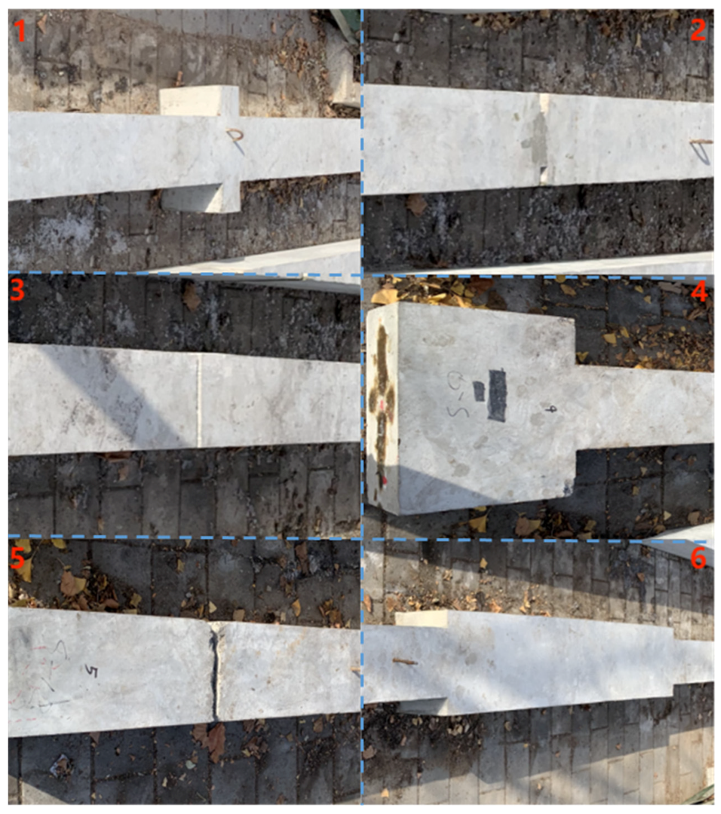
These model piles are constructed with concrete, and the measured propagation velocity of the stress wave c in the pile body is 4050 m/s. The standard pile section is a 250 × 250 mm square, and the pile length is 6 m. The pile number and the shape are shown in Table 2, and Figure 2 shows the photos of abnormal model piles. No. 0 is a complete pile with no change in the cross-sectional area. No. 2 and No. 3 are designed with the defects of different widths at different positions in the pile body. No. 5 is broken pile, and the fracture is connected by only 4 steel bars. The defects of the pile body are set in asymmetric positions to represent the different pile body defects, so the different curves can be measured from both ends of the pile, which is distinguished using A and B, as shown in Table 2.
Model pile No. 0 is a complete pile, so there is only 1 type of testing data related to it. Model piles No. 1 to No. 6 can be knocked from the A and B ends of the pile to obtain 2 different testing signals.

3.2. RNN+MLNN Analysis Model

RNN is a kind of recursive neural network that takes sequence data as input and makes recursion in the progression direction of the sequence, and all nodes are connected by a chain. RNN is very effective for the data with sequence characteristics. It can mine timing information and semantic information in data. By using this ability, the model based on RNN can make breakthroughs in solving the timing related problems such as speech recognition, stock price, weather forecast, language model, machine translation, etc. [47,48,49,50].
In order to generate LSPT signals, an external excitation source is required. The signal generated by the excitation source is directly reflected as the first peak in the curve, and the data points in this section impliedly contain some various information of the initial excitation, such as the strength of the hammer, the material of the hammerhead and the angle of the hit. The subsequent part of the curve is the result of both the initial excitation and the pile characteristics. From the perspective of the energy transfer, the vibration state sensed by the pile top sensor comes from the energy generated by excitation, firstly transmitted from the pile top to the pile bottom, then reflected to the pile top, and gradually sensed by the sensor. The velocity curve of the pile tip particle is a time-dependent curve with continuous amplitude. After A/D conversion, there is a sequential relationship in time and a continuous relationship in amplitude among the sampled points. The traditional neural network method extracts the time series waveform into several features, which become the time series irrelevant signals after being input to the model. In this process, the implied time features in the curve are lost. All these data have an important feature, that is, in addition to the general numerical characteristics of the input data, there is a sequential dimension [51,52]. Therefore, the RNN model is adopted to establish the analysis model of pile tip particle velocity data, which can not only consider the value relationship among the input features but also consider the order relationship among the input features. Since the testing data are timing series data, starting from excitation, the data analysis model is built with the RNN as the core.
The concept of deep learning originates from the research of artificial neural networks. Multi-layer perceptron with multiple hidden layers is a kind of deep learning structure [53]. The motivation for deep learning is to build neural networks that mimic human brains for analytical learning, which mimic human brain mechanisms to interpret data, such as images, sounds, and texts [54]. Deep learning combines low-level features to form more abstract high-level representation attribute categories or features to discover distributed feature representations of data. Compared with the traditional BP neural network, a deep learning neural network has a large increase in the number of network layers and the number of neural units. In this study, a multi-layer neural network (MLNN) is added on the basis of the RNN model by referring to the design idea of deep learning so as to dynamically adjust and select input features that have a great influence on the results.
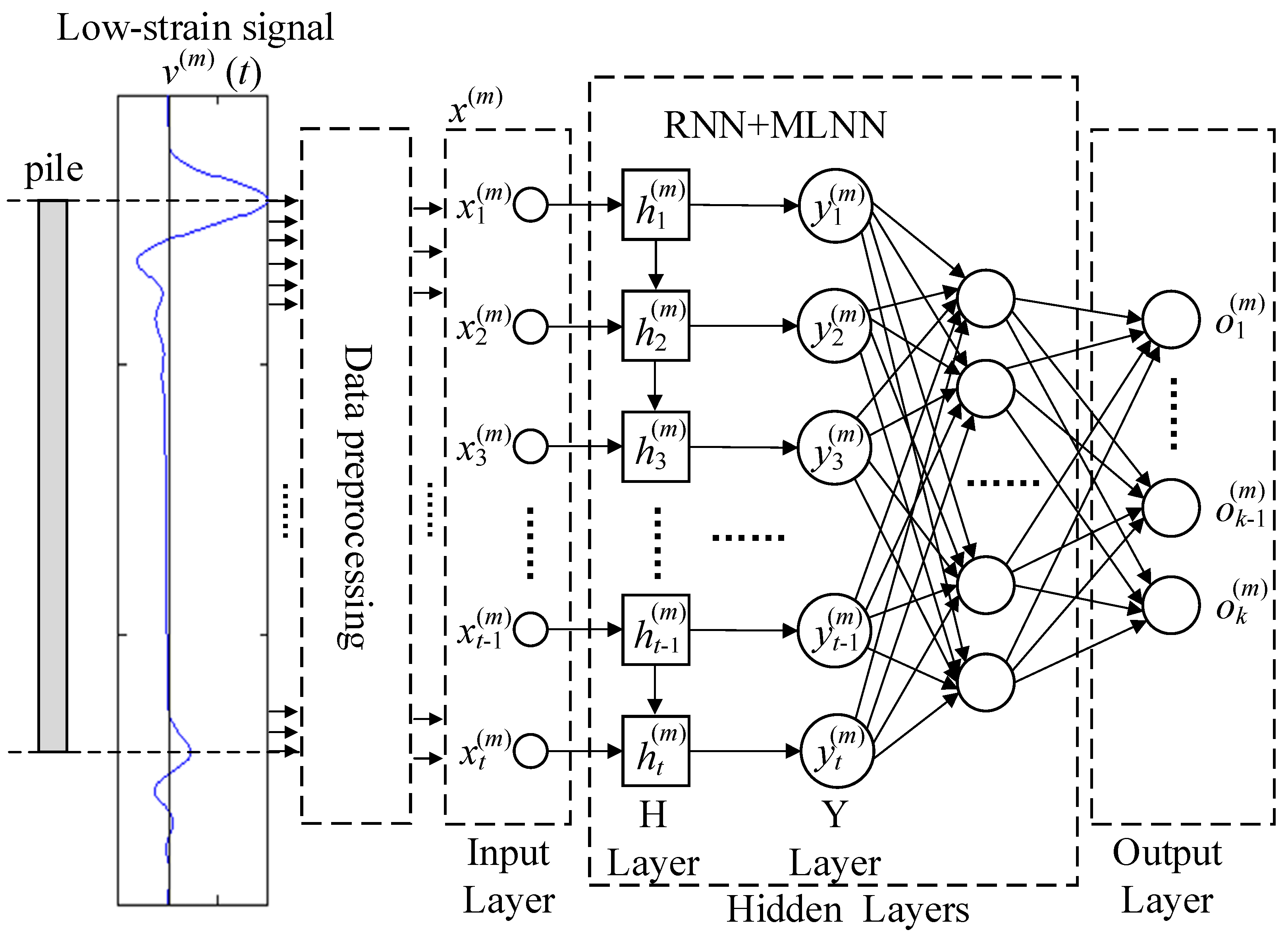
Combined with the MLNN model, the output results comprehensively consider multiple input features and their sequence relationships. A data analysis method (RNN+MLNN), based on the combination of RNN and MLNN, is proposed. The model structure is shown in Figure 3.
When a hand hammer is used to strike the pile head, the resulting stress waves propagate along the pile. At this time, the sensor at the pile top will collect the vibration velocity of the particle at the pile top, which is caused by the stress wave propagation along the pile, and the vibration velocity signal v(t) contains the change information of pile impedance.
For any velocity signal v m t , after the data acquisition by the dynamic measurement instrument with the sampling frequency f sample , this analog signal is converted to digital data. The subsequent data preprocessing processes the digital data into the input vector x 1 m , x 2 m , , x t m that meets the input requirements of the RNN model. Each value in the sequence is related to the excitation size and the pile impedance, that is, the numerical sequence contains the hidden state information about the pile impedance change.
For the low-strain testing data, the implicit state h t at any time t is related to the previous state h t 1 and the current input data x t . Taking tanh() as the activation function of neurons, the neuron model at time t in the RNN network can be expressed as Equation (3).
h t = tan h x t w x h + h t 1 w h h + b h
where w x h is the weight matrix from the input layer to the H layer, w h h is the weight matrix among the nodes in the H layer, and b h is the node bias in the H layer.
The output y t of the RNN network at time t can be expressed as Equation (4):
y t = tan h h t w h y + b y
where w h y is the weight matrix from the H layer to the Y layer, and b y is the node bias in the Y layer. y t contains the time series-related hidden features. The output of the Y layer is input into the MLNN, and the connection from the hidden features to the pile type classifications is established, as shown in Equation (5).
o = softmax y · w y o + b o
where w y o is the weight matrix from the Y layer to the output layer, and b o is the node bias in the output layer.
In actual testing items, the tested foundation piles need to be classified into 4 categories representing the different pile integrity, while in this experiment, we need to further classify these pile signals into 13 categories representing 13 different model piles. Therefore, this analysis model solves a classification problem. The different values of the output nodes are mapped to the probability distribution of [0, 1] by softmax(), and these probability values sum to 1. The category with the maximum classification probability is the corresponding classification result.
In this model, the output error adopts the multi-classification cross entropy loss function, as shown in Equation (6).
l o s s o , q = i o i log 2 q i
where i is the serial number of the pile type classification, q i is the probability that the data marked belongs to the type i, and o i is the probability belonging to the type i output by the model.
In the implementation of this RNN+MLNN model, two layers of RNN and two layers of neural network are adopted, and the specific network hierarchy is shown in Table 3. In order to avoid gradient disappearance and explosion in RNN, the deformable GRU model of RNN is used, which can achieve the equivalent effect and is easier to train. The first GRU layer uses 32 computing units and outputs the sequence values, the second GRU layer uses 64 computing units. The model results are output after a fully connected neural network with two layers [13,32]. In the last layer, the softmax() function is used to output the probabilities of 13 types, and the argmax() function is used to obtain the corresponding type number.
The parameters in this model include weight parameters w ( w x h , w h h , w h y , w y o ) and bias parameters b ( b h , b y , b o ). The Back Propagation (BP) algorithm is used to propagate the output error (the difference between the expected outputs and the actual outputs) calculated by the loss function [55]. In the process of back propagation, the output error is calculated back to the input layer through the hidden layers, according to the original path, and the error is distributed to each unit in each layer, the error data of each unit in each layer is obtained, and they are used as the basis for correcting the weight and the bias of each unit. The weight parameter w and the bias parameter b in the parameter list are updated according to the following Equations (7) and (8).
w = w λ l o s s w
b = b λ l o s s b
where λ is the learning rate and a hyper parameter that is manually set during the model training.
This calculation process uses the gradient descent method to complete. After constantly adjusting the weight and the bias of neuron units in each layer, the error data are reduced to a reasonable range. The actual calculation process can use a batch gradient descent algorithm, stochastic gradient descent algorithm, etc. [56,57].

3.3. Data Preprocessing

According to the “Technical Specification for Testing of Building Foundation Piles”, the following requirements are required for data collection: (1) The time domain data sampling points should not be less than 1024; (2) the sampling duration should be greater than 2 L/c + 5 ms; (3) the upper limit of the frequency range of amplitude-frequency data should not be less than 2000 Hz.
Therefore, the data sampling frequency and the sampling points are generally required in the testing site, as shown in Equations (9) and (10):
f r e sample 20   kHz
p o i n t _ l e n sample = 1024
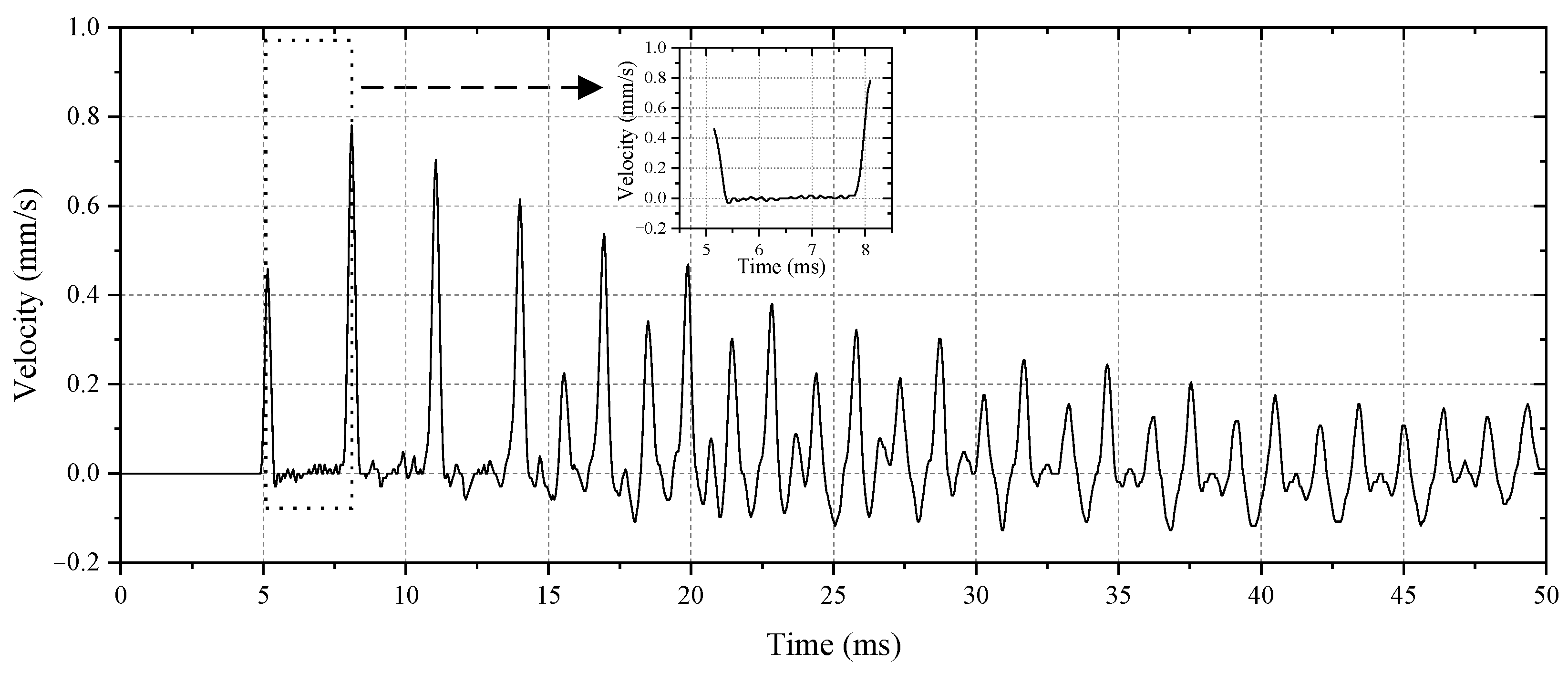
Due to the limited length of the model pile, the stress wave generated by hammering will oscillate forth and back in the pile body, forming multiple reflection peaks. This phenomenon is illustrated by the measured curve of the model pile No. 0, as shown in Figure 4. Before data analysis, the testing signal needs to be preprocessed, and the waveform between the excitation peak and the first reflection peak is intercepted for the analysis. At the same time, the data should be adjusted to match the input dimension of the RNN+MLNN analysis model.
The specific steps of data preprocessing are as follows:
(1) Identify the excitation peak. In the process of data sampling, the fluctuation of the excitation peak will be caused by the non-standard installation of sensors, the non-standard hit, and the incomplete treatment of pile top, so it is necessary to identify the initial edge of excitation first [58,59]. The initial edge and the peak detection algorithm is as follows (Algorithm 1):
Algorithm 1: The initial edge and the peak detection algorithm.
Inputs: v = v 1 , v 2 , , v n
Outputs: i n d e x rising ,   i n d e x max
1Calculate the average of the first part of num points v ¯ pre = 1 / n u m · 0 n u m 1 v i ;
2Form a new data sequence v , v = v v ¯ pre ;
3Calculate the maximum value of v , v max = max v ;
4Set the threshold value as v th = v max / th , th is the threshold parameter that can be manually set;
5Iterate over all data, starting from 1 until appearing:
v i < v i + 1 < v i + 2 and v i > v th
The order number i is the starting point of the initial edge: i n d e x rising = i ;
6Compute the differential sequence a of v , a i = v i v i 1 , i = 2 , 3 , 4 , , n ;
7Find the order number j where a j 0 a j + 1 < 0 after i n d e x rising , the j is the max value point i n d e x max = j ;
8Return i n d e x rising and i n d e x max ;
(2) Intercept the effective length. In this experiment, the stress wave velocity c and the pile length L are used to calculate the standard length. Firstly, the time t 2 l of the stress wave transmission from the pile top, to the pile bottom, and then back to the pile top is calculated, as shown in Equation (11). Equation (12) can be used to calculate the number of data points n 2 l collected during the t 2 l .
t 2 l = 2 × L / c
n 2 l = t 2 l × f r e sample
The data sequence with the effective length n 2 l , starting from i n d e x max , is intercepted from v and represented as v 2 l .
(3) Unify the dimensions of input features. Due to the differences in the sampling frequency, the experimental conditions, and the processing methods, the v 2 l from the different raw signals may become the data series with different lengths after step (2). The second order spline interpolation method [60] is used to unify the length of the data sequence into standard length t. The specific method is as follows:
For the sampled data sequence v 2 l , the partition of any two point interval [a,b] is ∆: a = s 1 < s 2 < < s n = b . s 1 , s n are called boundary points, s 2 ,…, s n 1 is the inner node, and the quadratic spline function corresponding to the partition ∆ is Equation (13):
s k = α 0 + α 1 k + α 2 2 ! k 2 + j = 1 n 1 β j 2 ! k k j + 2
where k k j + 2 = k < k j 2 , k k j 0 , k < k j , j = 1 , 2 , , n 1 , α i i = 0 , 1 , , h and β j j = 0 , 1 , , n 1 are arbitrary constants, which can be calculated by the boundary conditions.
After interpolation, the data sequence s with t points is formed, and the data dimension meets the input requirements of the RNN network.
(4) Normalize the value. All data sequence samples are normalized to the numerical interval [−1, 1]. The data with the largest absolute value in the data sequence is shown in Equation (14).
s max = max abs s
The newly generated data sequence x can be calculated by Equation (15) as follows:
x i = s i · 1 s max   i = 1 , 2 , , t
After steps (1) through (4), the data are clipping, adjusting, and converting from the raw data to a standardized list, and the input dimension meets the input requirements of RNN+MLNN model.

4. Experimental Process and Results

4.1. Data Acquisition

The model pile was barely placed on the ground, and the data was generated by knocking at both ends of the pile, as shown in Figure 5. In this asymmetric design, from the different starting point, a model pile can be regarded as two different types of piles. The pile dynamic measuring instrument BETC-C7, developed by China Academy of Building Research, was used to obtain the testing data by knocking at both ends [61].
There are seven model piles in total, among which six piles have asymmetric pile design and one complete pile. The 6 piles are tested from the 2 ends, respectively, and 12 types of testing data can be generated. Together with a complete pile, these field testing data can be divided into 13 types. In the experiment, 25 data samples were collected for each type of the model pile, 20 of which were used for training and validating, and 5 of which were used for testing, so the training set contains 260 data samples, and the test set contains 65 data samples.

4.2. Data Preparation

The testing signals collected by the pile DMI are usually binary signals in a special format. A series of transformations are required to form the input data dimensions required by the RNN model. The detailed steps are shown in Table 4.
As the sampling frequency was selected randomly at 20 kHz and 50 kHz in the collection process, the numbers of the data points obtained under the different sampling frequencies are different. The effective data points intercepted at 20 kHz are 60 points, and the effective data points intercepted at 50 kHz are 149 points.
The dimension of the input data is set to 64, so each input sample has 64 data points. After preprocessing the sampling data, the data set with the unified input feature dimension can be formed; specifically, the structure of the training data set is [64, 260], and the structure of the test data set is [64, 65].
The training data set D is divided into 10 mutually exclusive subsets with equal size by using the 10-fold cross validation method [62], that is,
D = D0∪D1…∪Di∪Dj…∪D9, Di∩Dj = Ø (ij)
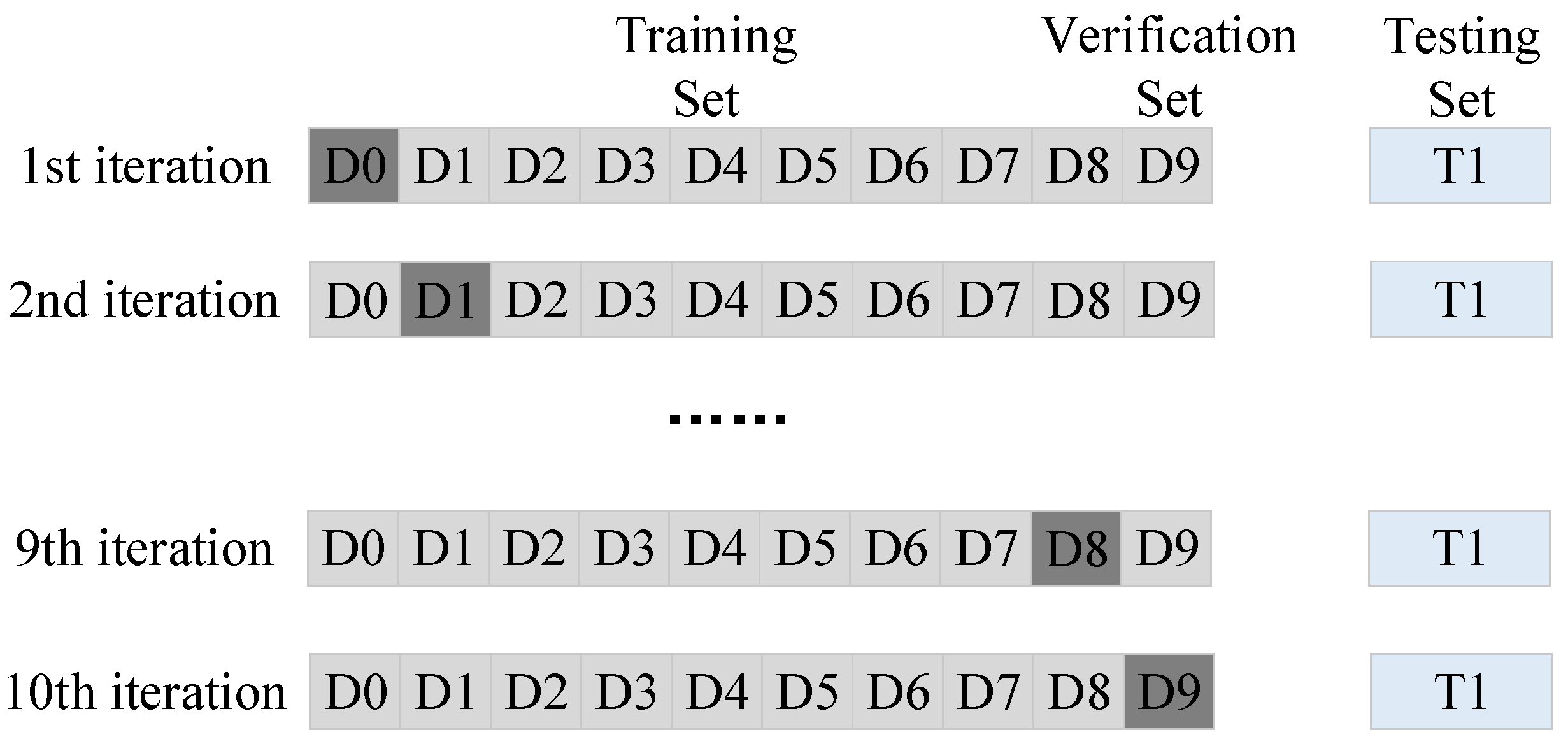
where one of them is selected as the verification set, and the other data sets are selected as the training set, as shown in Figure 6. The training process steps are as follows:
(1)
D0 is used as the verification set, and the rest, D1 to D9, are used as the training sets;
(2)
Repeat step (1) until each subset is used as a validation set;
(3)
Obtain 10 models with different training parameters and accuracy through steps (1) and (2);
(4)
Evaluate the model performance on the test data set T1;
(5)
Select the optimal model synthetically.

4.3. Test Results

The computer used for training the model is configured as follows: (1) CPU i7–12700 K with 12 cores and 20 threads; (2) graphics card NVIDIA GeForce RTX 3080 Ti 12 G; (3) memory 32 GB. In the training, the learning rate λ is set as 0.01, and a testing process is performed after each training. The result after 2000 iteration training and testing is shown in Figure 7.
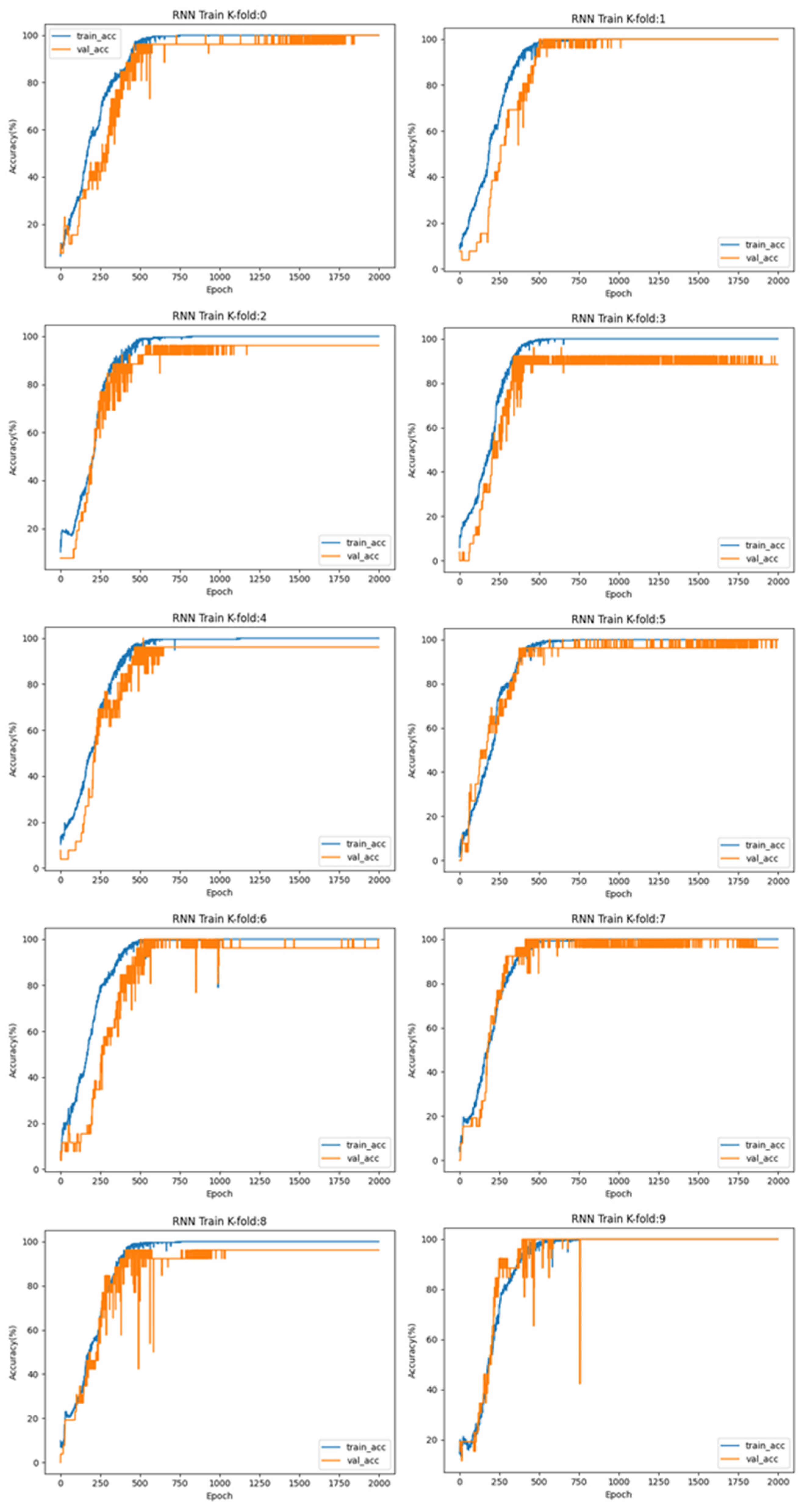
It can be seen from Figure 7 that each model in the training set has reached 100% accuracy in about 500 iterations, but the performance in the verification set is different. The accuracy of the second (K-fold:1) and the tenth (K-fold:9) iterations reached 100%, steadily, in the verification set. These two models are considered alternative models. Loading the data from the test set into 10 models generated by 10-fold cross validation, the performance of each model on the test set is shown in Figure 8.
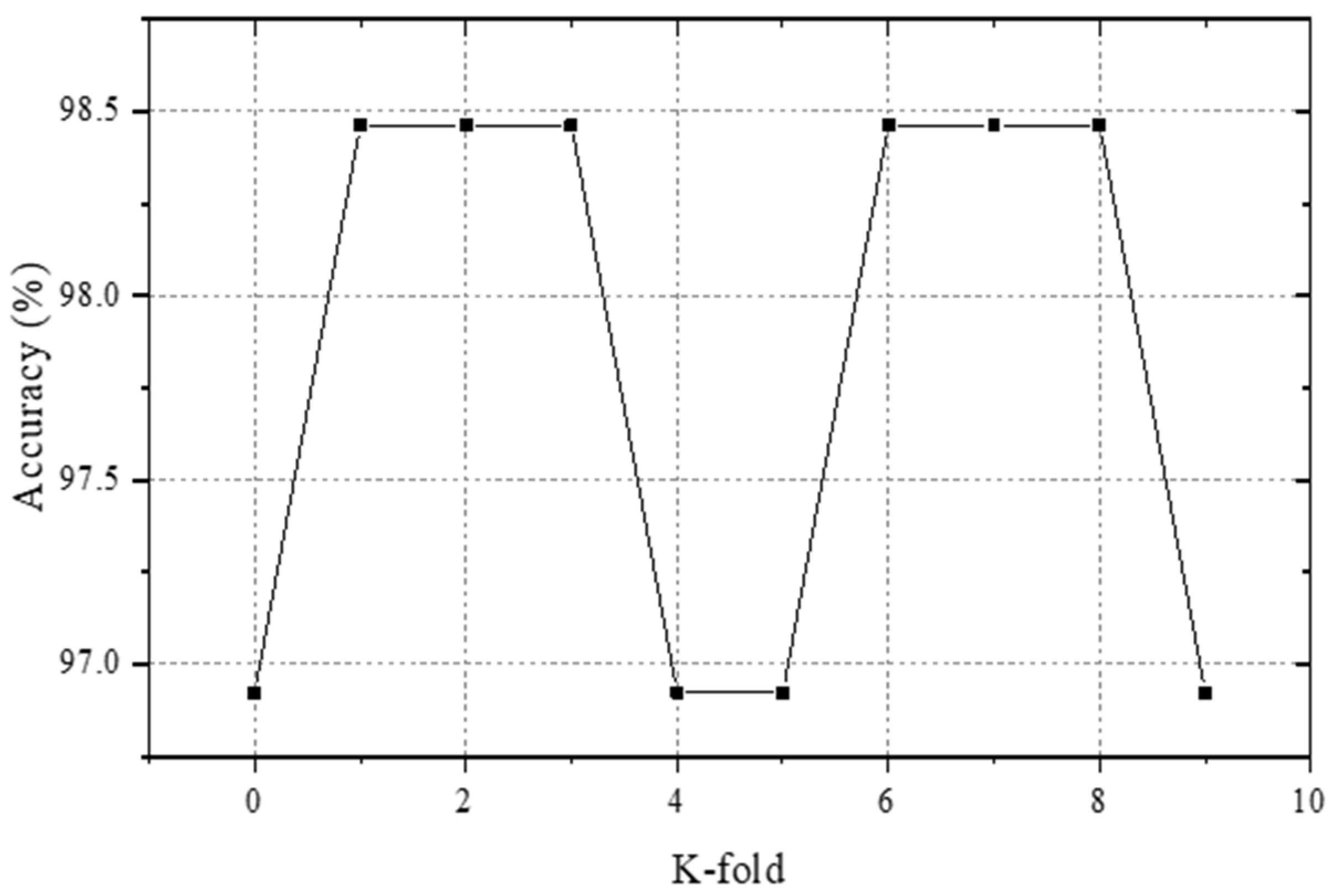
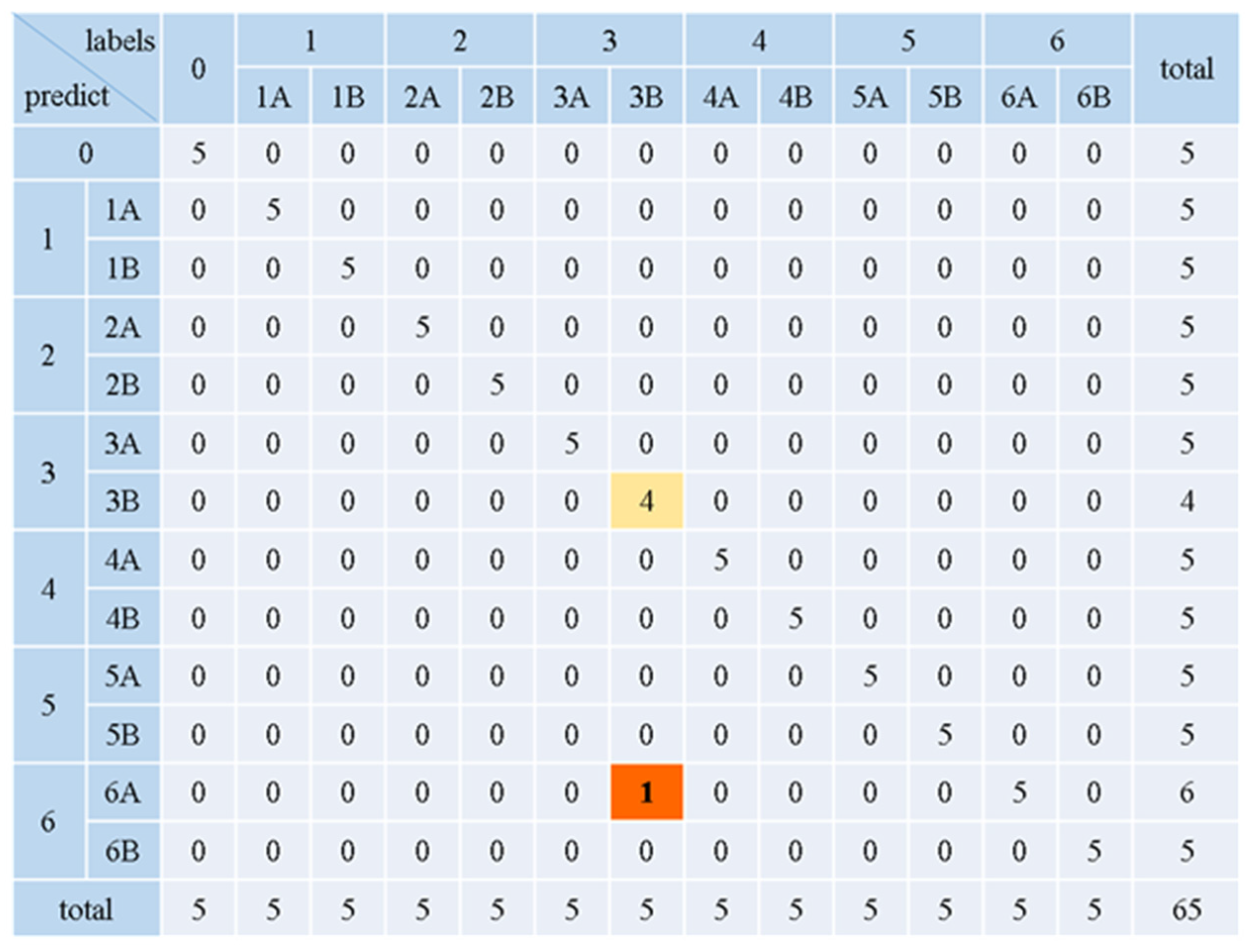
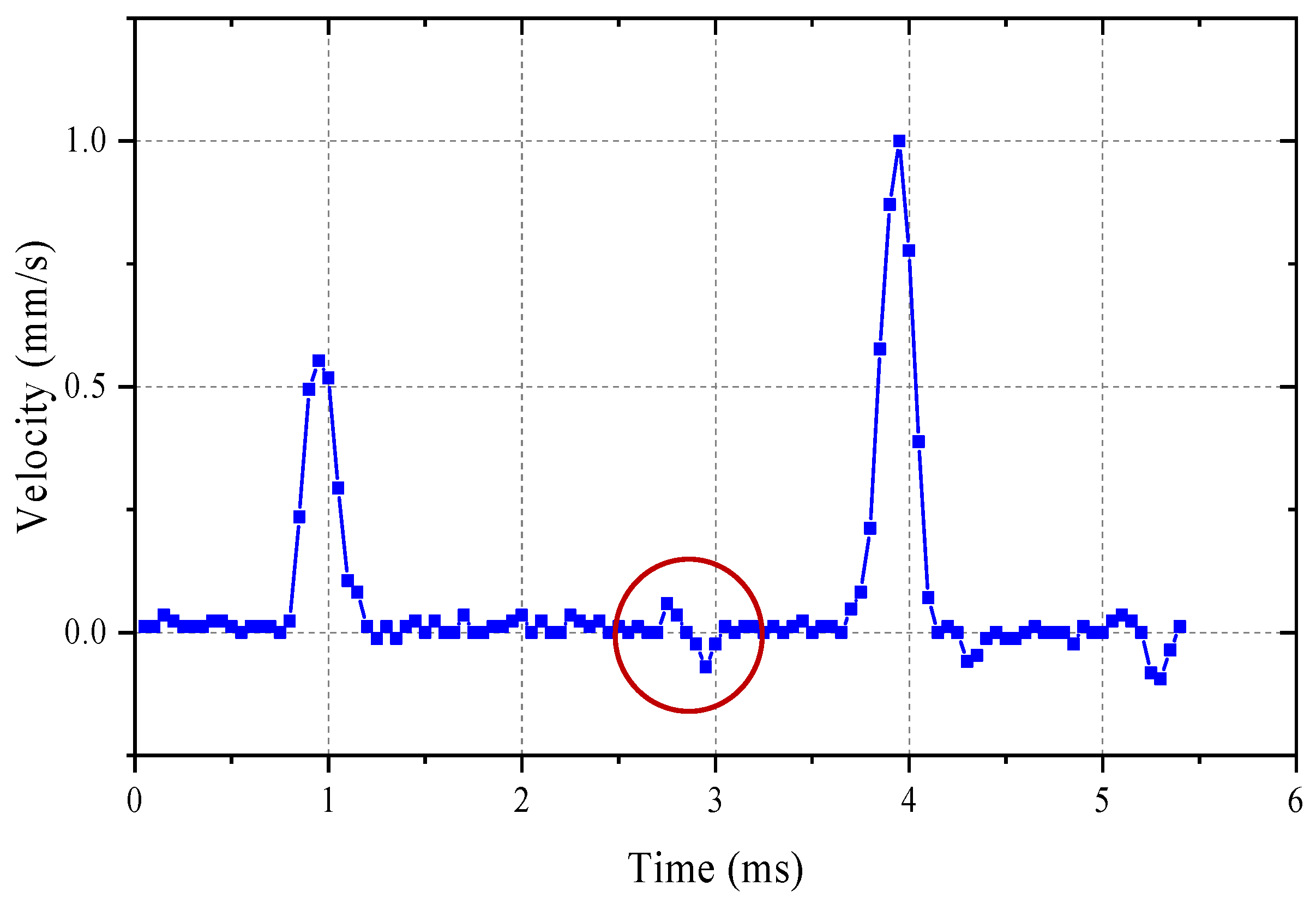
As can be seen from Figure 8, the model generated in K-fold:1 is judged to be the optimal model comprehensively, and the accuracy rate of this model in the test set reaches 98.46%. There are a total of 65 curve signals in the test set, and the model misclassifies one of them, as shown in Figure 9. A signal that should have been of type 3B was misclassified as 6A. Table 2 and Figure 3 show the appearance and the defect setting of the No. 3 pile. Pile No. 3 has the lightest defect degree among all piles. The testing signal curve obtained by hitting end B is shown in Figure 10. The red circle in Figure 10 shows the reaction of the pile defect in the curve. As the defect is shallow, the amplitude of curve change is also small, which is easy to ignore in the formation of features and the weight calculation, resulting in misjudgment. Neural network models express complex correlations between input and output features, but they do not have an intrinsic representation of causation, that is, input–output relationships are based on correlation rather than causation. This may lead to people not understanding how inputs produce outputs, thereby explaining why models are classified [63]. Similarly, the large number of parameters of neural network systems makes it difficult for even developers to annotate complex neural networks in an interpretable manner [64].
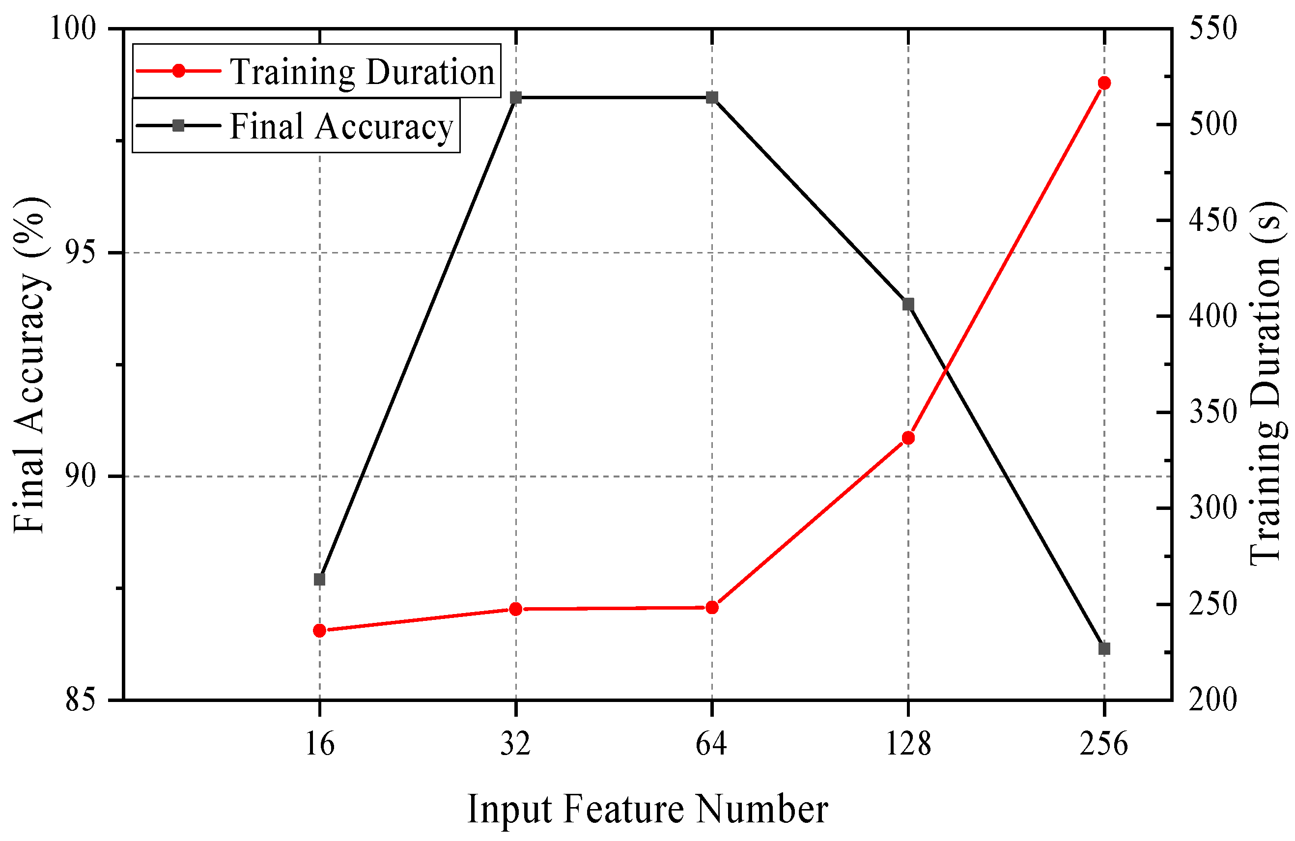
Reasonable selection of input features can improve the accuracy of the model [65]. The current 64 input features are obtained based on average sampling within the effective interval of the signal, so different input data dimensions contain different details. To verify whether adding input features will improve accuracy and test the influence of input time sequence data with different dimensions on this analysis model, we fitted the original data and extracted the input feature vectors with different dimensions, such as 16, 32, 64, 128, and 256. After 2000 training, the accuracy of the model, with different dimensions of data training on the same test set, is shown in Figure 11. In the test with different input dimensions, the final accuracy and the duration of 2000 training epochs are shown in Figure 12.
As can be seen from Figure 12, with the increase in input feature dimension, the model takes longer training time. However, the final accuracy of the model does not increase correspondingly. On the contrary, it has the highest accuracy when the input feature dimension is 32 and 64. It shows that simply increasing the dimension of input feature in the time domain has no positive effect on improving the accuracy, but it brings the cost of increased training time.
For comparison, we construct a single layer BP neural network (BPN) and a deep learning neural network (DL). The BPN has only one hidden layer, while the DL is a four-layer network with the structure of 32-64-32-13. Loading the same training set and the test set into the BPN and DL, respectively, and after 2000 iterations, the test result compared with the RNN+MLNN on the test set is shown in Figure 13. The BPN and the RNN+MLNN reach the optimal effect after about 620 iterations, and the DL reaches the optimal effect after about 1600 iterations.
The number of parameters in the three neural networks and their final accuracy on the test set are shown in Table 5. The accuracy of RNN+MLNN on the test set is higher than that of the other two models. This is because, with the same input feature dimension, the RNN network retains the time order of the input data and contains more information about the input data than the other two models. However, as a result, although the model has the same number of layers as the DL, it requires more training parameters and longer training time. Compared with the DL network and BPN network, the RNN network has some abnormal points with the multiple mutation of accuracy in the training process. The unique memory in RNN will affect other RNN nodes in the same time chain, so the gradient will be large and small at times, and the learning rate cannot be adjusted individually. As a result, the accuracy of RNN will mutate during the training process. However, with the progress of training, the parameters in the model gradually become stable, and the accuracy tends to be stable.

4.4. Discussion

In this study, RNN is used as the classification model, which improves the accuracy compared with the traditional BPN model and the simple use of the DL model. However, there is still a certain distance to apply the model to the actual testing field environment, which is mainly reflected in the following aspects:
(1)
Classification model aspect: Compared with other neural network models, the accuracy of RNN model on test set is improved, but the cost of the computing unit and the training time are increased. Some studies are also trying to unravel the relationship among neurons in the hidden layer of neural networks and form explainable details, but it is still difficult to explain the internal structure of artificial neural networks [66].
(2)
Input data characteristics: In this stage, the research mainly focuses on the simple combination of time series signals. The input features obtained from the time domain signals will also lose some information details due to the sampling interval. Subsequently, some experts in the foundation pile test are needed to help establish a data feature selection mechanism.
(3)
Training data: Since there are thousands of possibilities for the formation of LSPT data in reality, the size of training data will also affect the accuracy of the final model. We need different testing engineers to acquire more data, under different conditions, to form the training data set.
(4)
Model application scenarios: The test site of the foundation pile is a scene with pile–soil–human interaction, and each link will affect the final result. This study tries to reduce the relevant influencing factors as much as possible, and it attempts to establish a model with only two key testing factors, namely pile body and particle velocity. If this model is ever going to be put into practice, pile type, pile length, geological data, hammer material, and other factors need to be comprehensively considered, and input characteristics and model structure need to be further expanded on the basis of this research model. Although there is no data to prove that the pile type is related to the pile integrity, the foundation pile is a complex project, which may lead to pile integrity problems in the process of pile construction due to the different construction techniques of different pile types. This issue needs to be further studied on the basis of subsequent massive data collection.

5. Conclusions

The method of the low-strain pile test is a test technique commonly used in the site of the foundation pile test, and it has strong practicability because of its convenient and fast characteristics. However, the analysis of testing data and the pile classification have put forward higher requirements for testing personnel. In this paper, we try to use artificial intelligence to realize the pile classification based on the time series data. Through comparison, it is found that the accuracy of the model based on RNN+MLNN is improved compared with the similar use of the BP neural network and the deep learning neural network, but it requires longer training time and has more training parameters. The main contents of this paper include:
(1)
Model piles with different shapes are designed and processed to form LSPT signals for training and testing neural network models;
(2)
The RNN model is used to fully consider the timing attributes of input features;
(3)
The effective interval of input features is verified for the input timing features of different dimensions;
(4)
The advantage of using RNN in LSPT signal analysis is illustrated by comparing the RNN model with the traditional BP model and the DL model.
In the future, we will continue to expand the data set to the actual engineering piles, on the basis of this research, so as to really assist the field staff in the foundation pile testing site. It also avoids the situation of the schedule delay caused by the slowness of the testing process on site or the need for repeated testing caused by the misjudgment of testing data, it improves the efficiency and the reliability of the field testing of foundation pile engineering, and it reduces the burden of field engineers. In addition, it is necessary to continue to explore and test the new neural network model in order to achieve fewer training parameters and a shorter training time under the condition of maintaining high accuracy.

Author Contributions

Conceptualization, H.W.; methodology, H.W. and J.L.; software, H.W.; validation, H.W., S.Z., Y.Y. and F.Z.; formal analysis, H.W., F.Z. and J.L.; investigation, S.Z.; resources, S.Z.; data curation, H.W.; writing—original draft preparation, H.W.; writing—review and editing, H.W. and F.Z.; visualization, S.Z.; supervision, Y.Y.; project administration, Y.Y.; funding acquisition, Y.Y. All authors have read and agreed to the published version of the manuscript.

Funding

This research was funded by China Academy of Building Research Co., Ltd., grant number “20220112330730019”.

Data Availability Statement

All of the data, models, or code that support this study’s findings are available from the corresponding author upon reasonable request.

Conflicts of Interest

The authors declare no conflict of interest.

References

  1. Huang, Z.F.; Bai, X.H.; Yin, C.; Liu, Y.Q. Numerical analysis for the vertical bearing capacity of composite pile foundation system in liquefiable soil under sine wave vibration. PLoS ONE 2021, 16, e0248502. [Google Scholar]
  2. Wang, G.; Wang, G.; Shen, H.; Xu, G.H. An experimental study on the phase lags in response of pile base pressure to waves at different horizons with silty soil. Coastal Eng. 2012, 31, 21–32. [Google Scholar] [CrossRef]
  3. You, Y.; Wang, J.; Wu, Q.; Yu, Q.; Wang, X.; Guo, L. Causes of pile foundation failure in permafrost regions: The case study of a dry bridge of the Qinghai-Tibet Railway. Eng. Geol. 2017, 230, 95–103. [Google Scholar] [CrossRef]
  4. Zheng, J.J.; Liu, Y.; Guo, J.; Xu, Z.J. Probabilistic analysis and reliability assessment for acceptance rate of foundation pile testing. Chin. J. Geotech. Eng. 2009, 31, 1660–1664. [Google Scholar]
  5. Chen, F.; Jiao, H.; Han, L.; Shen, L.; Yu, G. Real-time monitoring of construction quality for gravel piles based on Internet of Things. Automat. Constr. 2020, 116, 103228. [Google Scholar] [CrossRef]
  6. Sun, G.; Kong, G.; Liu, H.; Amenuvor, A.C. Velocity response of model ballastless track XCC pile-raft foundation. Can. Geotech. J. 2017, 54, 1340–1345. [Google Scholar] [CrossRef]
  7. Li, G.S. Discussion on foundation pile test method and loading quantity in static load test. Build. Struct. 2020, 50, 118–129. [Google Scholar]
  8. Li, L.Z. Discussion about testing the bearing capacity of end bearing large-section in-situ concrete pile by core drilling method. Build. Sci. 2014, 30, 103–107. [Google Scholar]
  9. Zhang, Y.L.; Tang, D.G. Application of ultrasonic computerized tomography to diagnosis of pile construction integrity. Rock Soil Mech. 2009, 30, 3548–3552. [Google Scholar]
  10. Wu, B.J.; Wang, K.H.; Tong, W.F.; Xiao, S. Size effect and pile impedance variation in pile integrity test. Chin. J. Rock Mech. Eng. 2019, 38, 3230–3237. [Google Scholar]
  11. Zhao, S.; Wu, J.T.; Qiu, X.C. Study on defect detection of extended pile shaft under lateral low-strain integrity test. J. Zhejiang Univ. (Eng. Sci.) 2021, 55, 1867–1902. [Google Scholar]
  12. Fatehnia, M.; Amirinia, G. A review of Genetic Programming and Artificial Neural Network applications in pile foundations. Int. J. Geo-Eng. 2018, 9, 2. [Google Scholar] [CrossRef]
  13. Eftychios, P.; Marco, S.; Erika, P. A genetically optimized neural classifier applied to numerical pile integrity tests considering concrete piles. Comput. Struct. 2016, 162, 68–79. [Google Scholar]
  14. Sun, G.; Gu, Y. A pile testing method based on structural dynamic modification. Chin. J. Comput. Mech. 2004, 21, 5. [Google Scholar]
  15. Zhang, J.; Chen, L. Sonic echo test for pile integrity testing based on wavelet transform. J. Vib. Shock 2014, 33, 179–183. [Google Scholar]
  16. Wang, L.; Zhang, M.; Zhu, H.; Liu, Y. Review on artificial neural networks and their applications in geoscience. World Nucl. Geosci. 2021, 38, 15–26. [Google Scholar]
  17. Bai, X.Y.; Zhang, M.Y.; Kou, H.L.; Liu, H. Prediction of time effect of static pile bearing capacity by BP neural network. Geotech. Investig. Survey. 2014, 4, 7–12. [Google Scholar]
  18. Gao, L.; Xie, K. Application of artificial neural networks to geotechnical engineering. China Civil Eng. J. 2002, 35, 5. [Google Scholar]
  19. Jebur, A.A.; Atherton, W.; Al Khaddar, R.M.; Loffill, E. Artificial neural network (ANN) approach for modelling of pile settlement of open-ended steel piles subjected to compression load. Eur. J. Environ. Civil Eng. 2021, 25, 429–451. [Google Scholar] [CrossRef]
  20. Alzo’ubi, A.K.; Ibrahim, F. Predicting Loading–Unloading Pile Static Load Test Curves by Using Artificial Neural Networks. Geotech. Geol. Eng. 2018, 37, 1311–1330. [Google Scholar] [CrossRef]
  21. Wei, W.; Xie, H.; Mao, X.; Hu, H. Prediction of Bearing Capacity of Composite Foundation of Vibrating Gravel Pile Based on RBF Neural Network. In Proceedings of the 2019 IEEE 14th International Conference on Intelligent Systems and Knowledge Engineering (ISKE), Dalian, China, 14–16 November 2019. [Google Scholar]
  22. Goudjil, K.; Arabet, L. Assessment of deflection of pile implanted on slope by artificial neural network. Neural Comput. Appl. 2020, 33, 1091–1101. [Google Scholar] [CrossRef]
  23. He, Z.; Zhang, T.; Lee, R.B. VerIDeep: Verifying Integrity of Deep Neural Networks through Sensitive-Sample Fingerprinting. arXiv 2018. [Google Scholar] [CrossRef]
  24. Liu, R.; Zhao, Y.; Wei, S.; Yang, Y. Indexing of CNN Features for Large Scale Image Search. Pattern Recognit. 2018, 48, 2983–2992. [Google Scholar] [CrossRef]
  25. Yan, J.; Jin, L.; Yuan, Z.; Liu, Z. RNN for Receding Horizon Control of Redundant Robot Manipulators. IEEE Trans. Ind. Electron. 2022, 69, 1608–1619. [Google Scholar] [CrossRef]
  26. Wu, J.; Naggar, M.H.E.; Wang, K.H.; Liu, X. Analytical study of employing low-strain lateral pile integrity test on a de-fective extended pile shaft. J. Eng. Mech. 2020, 146, 04020103. [Google Scholar]
  27. Cosic, M.; Folic, B.; Folic, R. Numerical simulation of the pile integrity test on defected piles. Acta Geotech. Slovenica 2014, 11, 4–19. [Google Scholar]
  28. Zheng, C.; Kouretzis, G.P.; Ding, X.; Liu, H.; Poulos, H.G. Three-dimensional effects in low-strain integrity testing of piles: Analytical solution. Can. Geotech. J. 2016, 53, 225–236. [Google Scholar] [CrossRef]
  29. Chang, D.W.; Cheng, S.H.; Wang, Y.L. One-dimensional wave equation analyses for pile responses subjected to seismic horizontal ground motions. Soils Found. 2014, 54, 313–328. [Google Scholar] [CrossRef]
  30. Zheng, C.; Ding, X.; Sun, Y. Vertical vibration of a pipe pile in viscoelastic soil considering the three-dimensional wave effect of soil. Int. J. Geomech. 2016, 16, 04015037.1–04015037.10. [Google Scholar] [CrossRef]
  31. Qu, L.; Ding, X.; Zheng, C.; Liu, H. An analytical solution for wave propagation in a square pile due to transient point load. Comput. Geotech. 2017, 83, 77–82. [Google Scholar] [CrossRef]
  32. Ziółkowski, W.; Śliwiński, A. Application of a vibrational impedance head to the measurement of the complex elastic modulus by the driving point impedance method. Arch. Acoust. 1991, 16, 591–607. [Google Scholar]
  33. Ding, X.; Liu, H.; Liu, J.; Chen, Y. Wave propagation in a pipe pile for low-strain integrity testing. J. Eng. Mech. 2011, 137, 598–609. [Google Scholar] [CrossRef]
  34. Ertel, J.P.; Niederleithinger, E.; Grohmann, M. Advances in pile integrity testing. Near Surf. Geophys. 2016, 14, 503–512. [Google Scholar] [CrossRef]
  35. Lu, Z.T.; Wang, Z.L.; Liu, D.J. Study on low-strain integrity testing of pipe-pile using the elastodynamic finite integration technique. Int. J. Numer. Anal. Methods Geomech. 2013, 37, 536–550. [Google Scholar] [CrossRef]
  36. Alkhader, M.; Iyer, S.; Shi, W.; Venkatesh, T.A. Low frequency acoustic characteristics of periodic honeycomb cellular cores: The effect of relative density and strain fields. Compos. Struct. 2015, 133, 77–84. [Google Scholar] [CrossRef]
  37. Li, H.B.; Li, J.; Farhangi, V. Determination of piers shear capacity using numerical analysis and machine learning for gen-eralization to masonry large scale walls. Structures 2023, 49, 443–466. [Google Scholar] [CrossRef]
  38. Wang, C.; Zhang, W. A neural network model for diagnosing pile integrity based on reflection wave method. Rock Soil Mech. 2003, 24, 952–956. [Google Scholar]
  39. Liu, M.; Yue, X.; Yang, Y.; Li, Q. Intelligent identification of pile defect based on sym wavelet and bp neural network. Chin. J. Rock Mechanics Eng. 2007, 26, 5. [Google Scholar] [CrossRef]
  40. Pham, T.A.; Tran, V.Q.; Vu, H.L.T.; Ly, H.B. Design deep neural network architecture using a genetic algorithm for estimation of pile bearing capacity. PLoS ONE 2020, 15, e0243030. [Google Scholar] [CrossRef]
  41. Cui, D.M.; Yan, W.Z.; Wang, X.Q.; Lu, L.M. Towards intelligent interpretation of low strain pile integrity testing results using machine learning techniques. Sensors 2017, 17, 2443. [Google Scholar] [CrossRef]
  42. Jierula, A.; Oh, T.M.; Wang, S.; Lee, J.W. Detection of damage locations and damage steps in pile foundations using acoustic emissions with deep learning technology. Front. Struct. Civil Eng. 2021, 15, 15. [Google Scholar] [CrossRef]
  43. Zhang, P.Z.; Zhang, Y.C.; Song, X.G.; Yang, H.; Guo, Z.H.; Hu, Y. Modified calculation method of shaft friction for driven pile considering particle size effect. J. Shandong Univ. (Eng. Sci.) 2021, 51, 9. [Google Scholar]
  44. Yang, R.H. Application of model pile test in low strain inspection of foundation pile. Archit. Technol. 2015, 46, 562–565. [Google Scholar]
  45. Yang, W.G.; Ma, J.; Li, J.M.; Zhang, F.; Zhang, S.S. Discussion and analysis on the ability of testing pile integrity with low strain variation method. China Inspect. Body Lab. 2021, 29, 101–104. [Google Scholar] [CrossRef]
  46. Lai, J.; Yang, P.C.; Yang, B.H.; Chang, D.W. Integrity testing of model pile with embedded accelerometers. In Proceedings of the International Conference on Transportation Infrastructure and Materials (ICTIM 2017), Qingdao, China, 9–12 June 2017. [Google Scholar]
  47. Hu, Y.; Peng, X.; Yang, Z.; Jia, L.; Li, Y.J.; Xue, Q. Temporal representation learning for time series classification. Neural Comput. Appl. 2021, 33, 3169–3182. [Google Scholar] [CrossRef]
  48. Huesken, M.; Stagge, P. Recurrent neural networks for time series classification. Neurocomputing 2003, 50, 223–235. [Google Scholar] [CrossRef]
  49. Wei, C.; Kong, Z.; Yang, D.; Jia, Y.W.; Hill, D.J. Short-term residential load forecasting based on LSTM recurrent neural network. IEEE Trans. Smart Grid 2017, 10, 841–851. [Google Scholar]
  50. Liu, H.; Zhou, J.; Zheng, Y.; Jiang, W.; Zhang, Y. Fault diagnosis of rolling bearings with recurrent neural network-based auto encoders. ISA Trans. 2018, 77, 167–178. [Google Scholar] [CrossRef]
  51. Liang, H.T.; Liu, S.; Du, J.W.; Hu, Q.; Yu, X. Review of Deep Learning Applied to Time Series Prediction. J. Front. Comput. Sci. Technol. 2023, 1–21. [Google Scholar] [CrossRef]
  52. Huang, Y.; Han, X.; Zhao, L. Recurrent neural networks for complicated seismic dynamic response prediction of a slope system. Eng. Geol. 2021, 289, 106198. [Google Scholar] [CrossRef]
  53. Zhang, Q.; Yang, L.T.; Chen, Z.; Li, P. A survey on deep learning for big data. Inf. Fusion 2018, 42, 146–157. [Google Scholar] [CrossRef]
  54. Young, T.; Hazarika, D.; Poria, S.; Cambria, E. Recent Trends in Deep Learning Based Natural Language Processing. IEEE Computat. Intell. Mag. 2018, 13, 55–75. [Google Scholar] [CrossRef]
  55. Wang, L.; Zeng, Y.; Chen, T. Back propagation neural network with adaptive differential evolution algorithm for time series forecasting. Expert Syst. Appl. 2015, 42, 855–863. [Google Scholar] [CrossRef]
  56. Messaoud, S.; Bradai, A.; Moulay, E. Online GMM clustering and mini-batch-gradient descent based optimization for industrial IoT 4.0. IEEE Trans. Ind. Informat. 2020, 16, 1427–1435. [Google Scholar] [CrossRef]
  57. Shu, Y.; Huang, Y.; Li, B. Design of deep learning accelerated algorithm for online recognition of industrial products defects. Neural Comput. Appl. 2018, 31, 4527–4540. [Google Scholar] [CrossRef]
  58. Kim, J.Y.; Park, J.H.; Jang, S.Y.; Yang, J.R. Peak detection algorithm for vital sign detection using doppler radar sensors. Sensors 2019, 19, 1575. [Google Scholar] [CrossRef]
  59. Jiang, H.; Zhang, X.; Li, D.; Zhao, Y.; Zhang, Z. Multi-peak detection algorithm based on wavelength feature recognition in FBG sensor networks. Opt. Eng. 2021, 60, 106104. [Google Scholar] [CrossRef]
  60. Diaconu, D.C.; Bretcan, P.; Peptenatu, D.; Tanislav, D.; Mailat, E. The importance of the number of points, transect location and interpolation techniques in the analysis of bathymetric measurements. J. Hydrol. 2019, 570, 774–785. [Google Scholar] [CrossRef]
  61. Wang, H.; Zhang, Y.; Zhang, S.; Li, J.M. Design and implementation of low strain foundation pile dynamic tester. Electron. Des. Eng. 2019, 27, 5. [Google Scholar]
  62. Jung, K.; Bae, D.H.; Um, M.J.; Kim, S.; Jeon, S.; Park, D. Evaluation of Nitrate Load Estimations Using Neural Networks and Canonical Correlation Analysis with K-Fold Cross-Validation. Sustainability 2020, 12, 400. [Google Scholar] [CrossRef]
  63. Samek, W.; Binder, A.; Montavon, G.; Lapuschkin, S.; Muller, K.-R. Evaluating the Visualization of What a Deep Neural Network Has Learned. IEEE Trans. Neural Netw. Learn. Syst. 2016, 28, 2660–2673. [Google Scholar] [CrossRef] [PubMed]
  64. Marcus, G. Deep learning: A critical appraisal. arXiv 2018, arXiv:1801.00631. [Google Scholar]
  65. Liu, G.G.; Yang, Y.M.; Liu, B.; Zhong, D.Y.; Yang, S.Q. Prediction model of the bird strike risk in the airport sphere by using the artificial neural network. J. Saf. Environ. 2020, 20, 416–422. [Google Scholar]
  66. Mcgrath, T.; Kapishnikov, A.; Tomaev, N.; Pearce, A.; Hassabis, D.; Kim, B.; Paquet, U.; Kramnik, V. Acquisition of Chess Knowledge in AlphaZero. arXiv 2021, arXiv:2111.09259. [Google Scholar] [CrossRef] [PubMed]
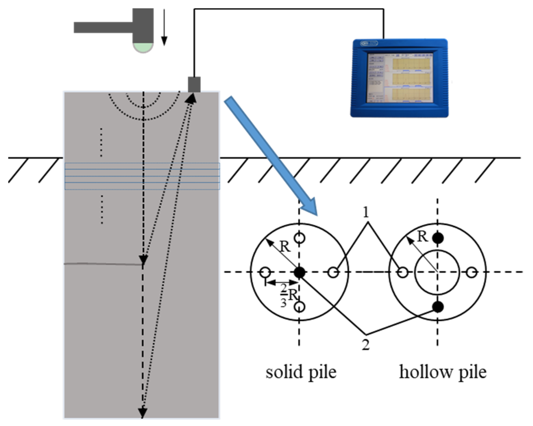
Figure 1. The schematic diagram of the low-strain dynamic test site.
Buildings 13 01228 g001
Figure 2. Photos of the abnormal model piles.
Buildings 13 01228 g002
Figure 3. The structure of the RNN+MLNN model.
Buildings 13 01228 g003
Figure 4. Testing data curve of the model pile No. 0.
Buildings 13 01228 g004
Figure 5. Testing the model pile in the field.
Buildings 13 01228 g005
Figure 6. The 10-fold cross validation method and test.
Buildings 13 01228 g006
Figure 7. Model accuracy curve on the training set and validation set.
Buildings 13 01228 g007
Figure 8. Model accuracy curve on the test set.
Buildings 13 01228 g008
Figure 9. Model labels and expected results graph.
Buildings 13 01228 g009
Figure 10. Signal from the B end of the No. 3 pile.
Buildings 13 01228 g010
Figure 11. Test accuracy under different input feature dimensions.
Buildings 13 01228 g011
Figure 12. Final accuracy and training duration under different input feature dimensions.
Buildings 13 01228 g012
Figure 13. The accuracy comparison among BPN, DL, and RNN+MLNN.
Buildings 13 01228 g013
Table 1. The number of features and the neural network structure in related research.
No.Paper
Author
Number of FeaturesModel Structure
1Wang et al. [38]68BP neural network, the input dimension is 68, the number of hidden layers is 1, the number of hidden layer nodes is 50, and the output dimension is 96. The activation function uses logarithmic Sigmoid function
2Liu et al. [39]4BP neural network, the input dimension is 4, the number of hidden layers is 1, the number of hidden layer nodes is 10, and the output dimension is 5. The activation function uses logarithmic Sigmoid function
3Tuan et al. [40]10Multilayer neural network, the input dimension is 10, the number of hidden layers is 4, the number of hidden layer nodes is (74, 17, 24, 12), and the output dimension is 1. The activation function uses relu function
4De-Mi et al. [41]21ELM, the input dimension is 4, the number of hidden layers is 1, the number of hidden layer nodes is 500, and the output dimension is 4. The activation function uses logarithmic Sigmoid function
5Alipujiang et al. [42]17Multilayer neural network, the input dimension is 17, the number of hidden layers is 2, the number of hidden layer nodes is (20, 20), and the output dimension is 2. The activation function uses logarithmic Sigmoid function
Table 2. Pile number and shape.
No.Pile Shape
0Buildings 13 01228 i001
1Buildings 13 01228 i002
2Buildings 13 01228 i003
3Buildings 13 01228 i004
4Buildings 13 01228 i005
5Buildings 13 01228 i006
6Buildings 13 01228 i007
Table 3. The specific network hierarchy of model RNN+MLNN.
No.Layer (Type)Output ShapeParam Number
1gru (GRU)(None, 16, 32)3360
2gru_1 (GRU)(None, 64)18,816
3dense (Dense)(None, 32)2080
4dense_1 (Dense)(None, 13)429
Total Params24,685
Table 4. Data preparation steps.
No.Processing StepMain ContentFeatures Number
1Acquire binary signalForms the binary data file by the DMI1024
2Convert dataConverts binary data to a numeric data array1024
3Identify excitation peakIdentify the excitation peak in 1024 data points1024
4Intercept the effective lengthIntercept the data points of 2 times the pile length from the data of 1024 points60 (20 kHz);
149 (50 kHz)
5Unify data dimensionUnify the data dimension into 64 by interpolation method64
6Normalize dataAdjust data value to [–1, 1]64
Table 5. The comparison of three neural networks.
No.TypeNetwork StructureTrainable ParametersDuration for 2000 Epochs (s)Final
Accuracy (%)
1BPN13845172.39528795.38
2DL32-64-32-136701211.30083996.92
3RNN+MLNN32-64-32-1324,685269.36060198.46
Disclaimer/Publisher’s Note: The statements, opinions and data contained in all publications are solely those of the individual author(s) and contributor(s) and not of MDPI and/or the editor(s). MDPI and/or the editor(s) disclaim responsibility for any injury to people or property resulting from any ideas, methods, instructions or products referred to in the content.